Hoang M. Le1 Cameron Voloshin1 Yisong Yue1
Abstract
When learning policies for real-world domains, two important questions arise: (i) how to effi-ciently use pre-collected off-policy, non-optimal behavior data; and (ii) how to mediate among dif-ferent competing objectives and constraints. We thus study the problem of batch policy learning un-der multiple constraints, and offer a systematic so-lution. We first propose a flexible meta-algorithm that admits any batch reinforcement learning and online learning procedure as subroutines. We then present a specific algorithmic instantiation and provide performance guarantees for the main ob-jective and all constraints. To certify constraint satisfaction, we propose a new and simple method for off-policy policy evaluation (OPE) and derive PAC-style bounds. Our algorithm achieves strong empirical results in different domains, including in a challenging problem of simulated car driv-ing subject to multiple constraints such as lane keeping and smooth driving. We also show exper-imentally that our OPE method outperforms other popular OPE techniques on a standalone basis, especially in a high-dimensional setting.
1. Introduction
We study the problem of policy learning under multiple con-straints. Contemporary approaches to learning sequential decision making policies have largely focused on optimizing some cost objective that is easily reducible to a scalar value function. However, in many real-world domains, choosing the right cost function to optimize is often not a straight-forward task. Frequently, the agent designer faces multiple competing objectives. For instance, consider the aspirational task of designing autonomous vehicle controllers: one may care about minimizing the travel time while making sure the driving behavior is safe, comfortable, or fuel efficient. Indeed, many such real-world applications require the pri-mary objective function be augmented with an appropriate
1
California Institute of Technology, Pasadena, CA. Correspon-dence to: Hoang M. Le<[email protected]>.
Technical report.
set of constraints (Altman,1999).
Contemporary policy learning research has largely focused on either online reinforcement learning (RL) with a focus on exploration, or imitation learning (IL) with a focus on learn-ing from expert demonstrations. However, many real-world settings already contain large amounts of pre-collected data generated by existing policies (e.g., existing driving behav-ior, power grid control policies, etc.). We thus study the complementary question: can we leverage this abundant source of (non-optimal) behavior data in order to learn se-quential decision making policies with provable guarantees on constraint satisfaction?
We thus propose and study the problem of batch policy learning under multiple constraints. Historically, batch RL is regarded as a subfield of approximate dynamic program-ming (ADP) (Lange et al.,2012), where a set of transitions sampled from the existing system is given and fixed. From an interaction perspective, one can view many online RL methods (e.g., DDPG (Lillicrap et al.,2016)) as running a growing batch RL subroutine per round of online RL. In that sense, batch policy learning is complementary to any exploration scheme. To the best of our knowledge, the study of constrained policy learning in the batch setting is novel. We present an algorithmic framework for learning sequential decision making policies from off-policy data. We employ multiple learning reductions to online and supervised learn-ing, and present an analysis that relates performance in the reduced procedures to the overall performance with respect to both the primary objective and constraint satisfaction. Constrained optimization is a well studied problem in su-pervised machine learning and optimization. In fact, our ap-proach is inspired by the work ofAgarwal et al.(2018) in the context of fair classification. In contrast to supervised learn-ing for classification, batch policy learnlearn-ing for sequential decision making introduces multiple additional challenges. First, setting aside the constraints, batch policy learning itself presents a layer of difficulty, and the analysis is signif-icantly more complicated. Second, verifying whether the constraints are satisfied is no longer as straightforward as passing the training data through the learned classifier. In sequential decision making, certifying constraint satisfac-tion amounts to an off-policy policy evaluasatisfac-tion problem, which is a challenging problem and the subject of active
research. In this paper, we develop a systematic approach to address these challenges, provide a careful error analysis, and experimentally validate our proposed algorithms. In summary, our contributions are:
• We formulate the problem of batch policy learning un-der multiple constraints, and present the first approach of its kind to solve this problem. The definition of constraints is general and can subsume many objec-tives. Our meta-algorithm utilizes multi-level learning reductions, and we show how to instantiate it using various batch RL and online learning subroutines. We show that guarantees from the subroutines provably lift to provide end-to-end guarantees on the original constrained batch policy learning problem.
• Leveraging techniques from batch RL as a subrou-tine, we provide a refined theoretical analysis for gen-eral non-linear function approximation that improves upon the previously known sample complexity bound (Munos & Szepesv´ari,2008) fromO(n4)toO(n2). • To evaluate and verify constraint satisfaction, we
pro-pose a simple new technique for off-policy policy eval-uation, which is used as a subroutine in our main algo-rithm. We show that it is competitive to other off-policy policy evaluation methods.
• We validate our algorithm and analysis with two ex-perimental settings. First, a simple navigation do-main where we consider safety constraint. Second, we consider a high-dimensional racing car domain with smooth driving and lane keeping constraints.
2. Problem Formulation
We first introduce notation. LetX⊂Rdbe a bounded and closedd-dimensional state space. LetAbe a finite action space. Letc: X×A7→[0, C]be the primary objective cost function that is bounded byC. Let there bemconstraint cost functions, gi : X×A 7→ [0, G], each bounded by
G. To simplify the notation, we view the set of constraints as a vector functiong : X×A 7→ [0, G]mwhereg(x, a) is the column vector of individualgi(x, a). Letp(·|x, a) denote the (unknown) transition/dynamics model that maps state/action pairs to a distribution over the next state. Let
γ ∈(0,1)denote the discount factor. Letχbe the initial states distribution.
We consider the discounted infinite horizon setting. An MDP is defined using the tuple(X,A, c, g, p, γ, χ). A pol-icy π ∈ Π maps states to actions, i.e., π(x) ∈ A. The value function Cπ : X 7→
R corresponding to the pri-mary cost functioncis defined in the usual way:Cπ(x) = E[P∞t=0γ
tc(x
t, at) | x0=x], over the randomness of the policyπand transition dynamicsp. We similarly define the vector-value function for the constraint costsGπ: X7→
Rm
as Gπ(x) =
E[P∞t=0γ tg(x
t, at)|x0=x]. DefineC(π) andG(π)as the expectation ofCπ(x)andGπ(x), respec-tively, over the distributionχof initial states.
2.1. Batch Policy Learning under Constraints
In batch policy learning, we have a pre-collected dataset,
D = {(xi, ai, x0i, c(xi, ai), g1:m(xi, ai)}ni=1, generated from (a set of) historical behavioral policies denoted jointly byπD. The goal of batch policy learning under constraints is to learn a policyπ∈ΠfromDthat minimizes the primary objective cost while satisfyingmdifferent constraints:
min
π∈Π C(π) s.t. G(π)≤τ
(OPT)
whereG(·) = [g1(·), . . . , gm(·)]>andτ ∈Rmis a vector of known constants. We assume that (OPT) is feasible. However, the datasetDmight be generated from multiple policies that violate the constraints.
2.2. Examples of Policy Learning with Constraints Counterfactual & Safe Policy Learning.In conventional online RL, the agent needs to “re-learn” from scratch when the cost function is modified. Our framework enables coun-terfactual policy learning assuming the ability to compute the new cost objective from the same historical data. A simple example issafepolicy learning (Garcıa & Fern´andez,
2015). Define safety costG(x, a) = φ(x, a, c)as a new function of existing costcand features associated with cur-rent state-action pair. The goal here is to counterfactually avoid undesirable behaviors observed from historical data. We experimentally study this safety problem in Section5. Other examples from the literature that belong to this safety perspective include planning under chance constraints (Ono et al.,2015;Blackmore et al.,2011). The constraint here is
G(π) =E[I(x∈Xerror)] = P(x∈Xerror)≤τ.
Multi-objective Batch Learning.Traditional policy learn-ing (RL or IL) presupposes that the agent optimizes a slearn-ingle cost function. In reality, we may want to satisfy multiple objectives that are not easily reducible to a scalar objective function. One example is learning fast driving policies un-der multiple behavioral constraints such as smooth driving and lane keeping consistency (see Section5).
2.3. Equivalence between Constraint Satisfaction and Regularization
Our constrained policy learning framework subsumes sev-eral existing regularized policy learning settings. Regular-ization typically encodes prior knowledge, and has been used extensively in the RL and IL literature to improve learning performance. Many instances of regularized policy learning can be naturally cast into (OPT):
• Entropy regularized RL(Haarnoja et al.,2017;Ziebart,
2010) is equivalent toG(π) = H(π), where H(π)
measures policy entropy.
• Smooth imitation learning(Le et al.,2016) is equiva-lent toG(π) = minh∈H∆(h, π), whereHis a class of provably smooth policies and∆is a divergence metric. • Regularizing RL with expert demonstration ( Hes-ter et al., 2018) is equivalent to G(π) =
E[`(π(x), π∗(x))], whereπ∗is the expert policy. • Conservative policy improvement(Levine & Abbeel,
2014;Schulman et al.,2015;Achiam et al.,2017) is equivalent toG(π) =DKL(π, πk), whereπkis some “well-behaving” policy.
We provide a detailed equivalence derivation of the above examples in AppendixA. Of course, some problems are more naturally described using the regularization perspec-tive, while others using constraint satisfaction.
More generally, one can establish the equivalence between regularized and constrained policy learning via a simple appeal to Lagrangian duality as shown in Proposition2.1
below. This Lagrangian duality also has a game-theoretic interpretation (Section 5.4 ofBoyd & Vandenberghe(2004)), which serves as an inspiration for developing our approach. Proposition 2.1. Let Π be a convex set of policies. Let
C: Π7→R, C: Π7→RKbe value functions. Consider the two policy optimization tasks:
Regularization: min
π∈Π C(π) +λ >G(π)
Constraint: min
π∈Π C(π) s.t.G(π)≤τ Assume that the Slater’s condition is satisfied in the
Constraint problem (i.e., ∃π s.t. G(π) < τ). As-sume also that the constraint cannot be removed with-out changing the optimal solution, i.e., infπ∈ΠC(π) <
infπ∈Π:G(π)≤τC(π). Then∀λ > 0,∃τ, and vice versa, such that Regularizationand Constraintshare the same optimal solutions. (Proof in AppendixA.)
3. Proposed Approach
To make use of strong duality, we firstconvexifythe policy classΠ by allowing stochastic combinations of policies, which effectively expandsΠinto its convex hullConv(Π). Formally,Conv(Π)containsrandomized policies,1which we denoteπ=PT
t=1αtπtforπt∈ΠandP T
t=1αt = 1. Executing a mixedπconsists of first samplingonepolicy
πtfromπ1:T according to distributionα1:T, and then exe-cutingπt. Note that we still haveE[π] =PTt=1αtE[πt]for any first-moment statistic of interest (e.g., state distribution, expected cost). It is easy to see that the augmented version
1
This places no restrictions on the individual policies. Individ-ual policies can be arbitrarily non-convex. Convexifiying a policy class amounts to allowing ensembles of learned policies.
Algorithm 1Meta-algo for Batch Constrained Learning 1: foreach roundtdo
2: πt←Best-response(λt)
3: πbt← 1tPtt0=1πt0,bλt←1tPtt0=1λt0 4: Lmax= maxλL(bπt, λ)
5: Lmin=L(Best-response(bλt),bλt)
6: ifLmax−Lmin≤ωthen 7: Returnbπt
8: λt+1←Online-algorithm(π1, . . . , πt−1, πt)
of (OPT) overConv(Π)has a solution at least as good as the original (OPT). As such, to lighten the notation, we will equateΠwith its convex hull for the rest of the paper. 3.1. Meta-Algorithm
The Lagrangian of (OPT) isL(π, λ) =C(π) +λ>(G(π)−
τ)forλ∈Rm+. Clearly (OPT) is equivalent to the min-max problem:min
π∈Πλmax∈Rk
+
L(π, λ). We assume (OPT) is feasible and that Slater’s condition holds (otherwise, we can simply increase the constraintτby a tiny amount). Slater’s con-dition and policy class convexification ensure that strong duality holds (Boyd & Vandenberghe,2004), and (OPT) is also equivalent to the max-min problem:max
λ∈Rk
+
min
π∈ΠL(π, λ). SinceL(π, λ)is linear in bothλandπ, strong duality is also a consequence of von Neumann’s celebrated convex-concave minimax theorem for zero-sum games (Von Neu-mann & Morgenstern,2007). From a game-thoeretic per-spective, the problem becomes finding the equilibrium of a two-player game between theπ−player and theλ−player (Freund & Schapire, 1999). In this repeated game, the
π−player minimizesL(π, λ)given the currentλ, and the
λ−player maximizes it given the current (mixture over)π. We first present a meta-algorithm (Algorithm1) that uses any no-regret online learning algorithm (forλ) and batch policy optimization (forπ). At each iteration, givenλt, the
π-player runsBest-responseto get the best response:
Best-response(λt) = arg min π∈Π
L(π, λt)
= arg min
π∈Π
C(π) +λ>t(G(π)−τ).
This is equivalent to a standard batch reinforcement learn-ing problem where we learn a policy that is optimal with respect toc+λ>tg. The corresponding mixed strategy is the uniform distribution over all previousπt. In response to the
π−player, theλ−player employsOnline-algorithm, which can beanyno-regret algorithm that satisfies:
X t L(πt, λt)≥max λ X t L(πt, λ)−o(T) Finally, the algorithm terminates when the estimated primal-dual gap is below a thresholdω(Lines 7-8).
Algorithm 2Constrained Batch Policy Learning
Input: DatasetD ={xi, ai, x0i, ci, gi}ni=1 ∼πD. Online algo-rithm parameters:`1norm boundB, learning rateη
1: Initializeλ1= (mB+1, . . . ,mB+1)∈Rm+1 2: foreach roundtdo
3: Learnπt←FQI(c+λt>g) //FQI with costc+λ>tg
4: EvaluateCb(πt)←FQE(πt, c) //Algo3withπt, costc
5: EvaluateGb(πt)←FQE(πt, g) //Algo3withπt, costg
6: πbt← 1 t Pt t0=1πt0 7: Cb(bπt)←1tPtt0=1Cb(πt0),Gb(πbt)← 1tPtt0=1Gb(πt0) 8: λbt← 1tPtt0=1λt0
9: Learnπe←FQI(c+bλt>g) //FQI with costc+bλ>tg
10: EvaluateCb(eπ)←FQE(eπ, c),Gb(eπ)←FQE(eπ, g)
11: bLmax= max λ,kλk1=B b C(πbt) +λ> h (Gb(πbt)−τ)>,0 i> 12: bLmin=Cb(eπ) +λb > t h (Gb(πe)−τ) > ,0i >
13: ifLbmax−bLmin≤ωthen 14: Returnbπt 15: Setzt= h (Gb(πt)−τ)>,0 i> ∈Rm+1 16: λt+1[i] =B λt[i]e −ηzt[i] P jλt[j]e−ηzt[j]∀i //λ[i]thei th coordinate
Algorithm 1 is guaranteed to converge assuming: (i)
Best-responsegives the best single policy in the class, and (ii)LmaxandLmincan be evaluated exactly.
Proposition 3.1. Assuming (i) and (ii) above, Algorithm1
is guaranteed to stop and the convergence depends on the regret ofOnline-algorithm. (Proof in AppendixB.) 3.2. Our Main Algorithm
We now focus on a specific instantiation of Algorithm1. Algorithm2is our main algorithm in this paper.
Policy Learning. We instantiateBest-responsewith Fitted Q Iteration (FQI), a model-free off-policy learning approach (Ernst et al., 2005). FQI relies on a series of reductions to supervised learning. The key idea is to ap-proximate the true action-value functionQ∗by a sequence {Qk ∈F}Kk=0, whereFis a chosen function class. In Lines 3 & 9,FQI(c+λ>g)is defined as follows. With
Q0randomly initialized, for eachk= 1, . . . , K, we form a new training datasetDek ={(xi, ai), yi}ni=1where:
∀i: yi= (ci+λ>gi) +γmin
a Qk−1(x 0 i, a), and(xi, ai, xi0, ci, gi)∼D(original dataset). A supervised regression procedure is called to solve for:
Qk= arg min f∈F 1 n n X i=1 (f(xi, ai)−yi)2. The policy then:πK= arg minaQK(·, a).
FQI has been shown to work well with several empirical domains: spoken dialogue systems (Pietquin et al.,2011), physical robotic soccer (Riedmiller et al.,2009), and
cart-Algorithm 3Fitted Off-Policy Evaluation with Function Approximation:FQE(π, c)
Input: DatasetD ={xi, ai, x0i, ci}ni=1∼πD. Function classF. Policyπto be evaluated 1: InitializeQ0∈Frandomly 2: fork= 1,2, . . . , Kdo 3: Compute targetyi=ci+γQk−1(x0i, π(x 0 i)) ∀i
4: Build training setDek={(xi, ai), yi}ni=1 5: Solve a supervised learning problem:
Qk= arg min f∈F 1 n Pn i=1(f(xi, ai)−yi) 2 Output: Cbπ(x) =QK(x, π(x)) ∀x
pole swing-up (Riedmiller,2005). Another possible model-free subroutine is Least-Squares Policy Iteration (LSPI) (Lagoudakis & Parr,2003). One can also consider model-based alternatives (Ormoneit & Sen,2002).
Off-policy Policy Evaluation. A crucial difference be-tween constrained policy learning and existing work on constrained supervised learning is the technical challenge of evaluating the objective and constraints. First, esti-mating Lb(π, λ) (Lines 11-12) requires estimating Cb(π) and Gb(π). Second, any gradient-based approach to
Online-learningrequires passing inGb(π)−τas part of gradient estimate (line 15). This problem is known as the off-policy policy evaluation (OPE) problem: we need to evaluateCb(π)andGb(π)having only access to dataD∼πD There are three main contemporary approaches to OPE: (i) importance weighting (IS) (Precup et al.,2000;2001), which is unbiased but often has high-variance; (ii) regression-based direct methods (DM), which are typically model based (Thomas & Brunskill,2016),2and can be bi-ased but have much lower variance than IS; and (iii) doubly-robust techniques (Jiang & Li,2016;Dud´ık et al.,2011), which combine IS and DM.
We propose a new and simple model-free technique using function approximation, called Fitted Q Evaluation (FQE). FQE is based on an iterative reductions scheme similar to FQI, but for the problem of off-policy evaluation. Algorithm
3lays out the steps. The key difference with FQI is that theminoperator is replaced byQk−1(x0i, π(x0i))(Line 3 of Algorithm3). Eachx0icomes from the originalD. Since we knowπ(x0i), eachDekis well-defined. Note that FQE can be plugged-in as a direct method if one wishes to augment the policy evaluation with a doubly-robust technique.
Online Learning Subroutine. AsL(πt, λ)is linear inλ, many online convex optimization approaches can be used forOnline-algorithm. Perhaps the simpliest choice is Online Gradient Descent (OGD) (Zinkevich,2003). We include an instantiation using OGD in AppendixG.
2
I.e., using regression to learn the reward function and transi-tion dynamics model, before solving the estimated MDP.
For our main Algorithm2, similar to (Agarwal et al.,2018), we use Exponentiated Gradient (EG) (Kivinen & Warmuth,
1997), which has a regret bound ofO(plog(m)T)instead ofO(√mT)as in OGD. One can view EG as a variant of Online Mirror Descent (Nemirovsky & Yudin,1983) with a softmax link function, or of Follow-the-Regularized-Leader with entropy regularization (Shalev-Shwartz et al.,2012). Gradient-based algorithms generally require boundedλ. We thus forcekλk1 ≤ B using hyperparameterB. Solving (OPT) exactly requiresB=∞. We will analyze Algorithm
2with respect to finiteB. With some abuse of notation, we augmentλinto a(m+1)−dimensional vector by appending
B − kλk1, and augment the constraint cost vectorg by appending0(Lines 11, 12 & 15 of Algorithm2).3
4. Theoretical Analysis
4.1. Convergence GuaranteeThe convergence rate of Algorithm2depends on the radius
Bof the dual variablesλ, the maximal constraint valueG, and the number of constraintsm. In particular, we can show
O(Bω22)convergence for primal-dual gapω.
Theorem 4.1(Convergence of Algorithm2). AfterT itera-tions, the empirical duality gap is bounded by
b
Lmax−Lbmin≤2
Blog(m+ 1)
ηT + 2ηBG
2 Consequently, to achieve the primal-dual gap ofω, setting
η = ω
4G2B will ensure that Algorithm2converges after
16B2G2log(m+1)
ω2 iterations. (Proof in AppendixB.)
Convergence analysis of our main Algorithm2is an exten-sion of the proof to Proposition3.1, leveraging the no-regret property of the EG procedure (Shalev-Shwartz et al.,2012).
4.2. Generalization Guarantee of FQE and FQI In this section, we provide sample complexity analysis for FQE and FQI asstandaloneprocedures for off-policy evaluation and off-policy learning. We use the notion of pseudo-dimension as capacity measure of non-linear func-tion classF (Friedman et al.,2001). Pseudo-dimension
dimF, which naturally extends VC dimension into the re-gression setting, is defined as the VC dimension of the function class induced by the sub-level set of functions ofF:
dimF = VC-dim({(x, y)7→ sign(f(x)−y) :f ∈ F}). Pseudo-dimension is finite for a large class of function ap-proximators. For example,Bartlett et al.(2017) bounded the pseudo-dimension of piece-wise linear deep neural networks (e.g., with ReLU activations) asO(W LlogW), whereW
is the number of weights, andLis the number of layers. 3
The(m+ 1)th
coordinate ofgis thus always satisfied. This augmentation is only necessary when executing EG.
Both FQI and FQE rely on reductions to supervised learning to update the value functions. In both cases, the learned policy and evaluation policy induces a different state-action distribution compared to the data generating distributionµ. We use the notion of concentration coefficient for the worst case, proposed by (Munos,2003), to measure the degree of distribution shift. The following standard assumption from analysis of related ADP algorithms limits the severity of distribution shift over future time steps:
Assumption 1(Concentration coefficient of future state-ac-tion distribustate-ac-tion). (Munos, 2003; 2007; Munos & Szepesv´ari,2008;Antos et al.,2008a;b;Lazaric et al.,2010;
2012;Farahmand et al.,2009;Maillard et al.,2010) Let Pπ be the operator acting on f : X×A 7→
Rs.t.
(Pπf)(x, a) =R Xf(x
0, π(x0))p(dx0|x, a). Given data gen-erating distributionµ, initial state distributionχ, form≥0
and an arbitrary sequence of stationary policies{πm}m≥1 define the concentration coeffient:
βµ(m) = sup π1,...,πm d(χPπ1Pπ2. . . Pπm) dµ ∞ We assumeβµ= (1−γ)2 P m≥1 mγm−1β µ(m)<∞. This assumption is valid for a fairly large class of MDPs (Munos,2007). For instanceβµis finite for any finite MDP, or any infinite state-space MDP with bounded transition density.4 Having a finite concentration coefficient is
equiva-lent the top-Lyapunov exponentΓ≤0(Bougerol & Picard,
1992), which means the underlying stochastic system is stable. We show below a simple sufficient condition for Assumption1(albeit stronger than necessary).
Example 4.1. Consider an MDP such that for any non-stationary distributionρ, the marginals over states satisfy
ρx(x)
µx(x) ≤L(i.e., transition dynamics are sufficiently
stochas-tic), and∃M : ∀x, a : µ(a|x) > M1 (i.e., the behavior policy is sufficiently exploratory). Thenβµ≤LM. Recall that for a given policy π, the Bellman (evalua-tion) operator is defined as (TπQ)(x, a) = r(x, a) +
γR XQ(x
0, π(x0))p(dx0|x, a). In general
Tπf may not be-long toFforf ∈F. For FQE (and FQI), the main operation in the algorithm is to iteratively projectTπQk−1back toF viaQk = arg minf∈Fkf −TπQk−1k. The performance of both FQE and FQI thus depend on how well the function classFapproximates the Bellman operator. We measure the ability of function classFto approximate the Bellman evaluation operator via the worst-case Bellman error:
4
This assumption ensures sufficient data diversity, even when the executing policy is deterministic. An example of how learning can fail without this assumption is based on the “combination lock” MDP (Koenig & Simmons,1996). In this deterministic MDP example,βµcan grow arbitrarily large, and we need an exponential
Definition 4.1(inherent Bellman evaluation error). Given a function class F and policy π, the inherent Bell-man evaluation error of F is defined as dπ
F =
supg∈Finff∈Fkf−Tπgkπ where k·kπ is the `2 norm weighted by the state-action distribution induced byπ. We are now ready to state the generalization bound for FQE: Theorem 4.2 (Generalization error of FQE). Under As-sumption1, for >0&δ∈ (0,1), afterK iterations of Fitted Q Evaluation (Algorithm3), forn=O C24(log
K δ + dimFlogC 2 2+logdimF)
, we have with probability1−δ:
C(π)−Cb(π) ≤ γ1/2 (1−γ)3/2 p βµ(2dπF+) + 2γK/2C (1−γ)1/2 .
This result shows a dependency onofOe(12), compared
to Oe(14)from other related ADP algorithms (Munos &
Szepesv´ari,2008;Antos et al.,2008b). The price that we pay is a multiplicative constant 2 in front of the inherent errordπ
F. The error from second term on RHS decays exponentially with iterationsK. The proof is in AppendixE.
We can show an analogous generalization bound for FQI. While FQI has been widely used, to the best of our knowl-edge, a complete analysis of FQI for non-linear function approximation has not been previously reported.5
Definition 4.2(inherent Bellman optimality error). (Munos & Szepesv´ari, 2008) Recall that the Bellman optimal-ity operator is defined as (TQ)(x, a) = r(x, a) +
γR
Xmina0∈AQ(x
0, a0)p(dx0|x, a). Given a function class
F, the inherent Bellman error is defined as dF =
supg∈Finff∈Fkf−Tgkµ, where k·kµ is the `2 norm weighted byµ, the state-action distribution induced byπD. Theorem 4.3(Generalization error of FQI). Under Assump-tion1, for > 0 &δ ∈ (0,1), afterK iterations of Fit-ted Q Iteration, for n = O C24(log
K δ +dimFlogC 2 2 + logdimF)
, we have with probability1−δ: C∗−C(πK) ≤ 2γ (1−γ)3 p βµ(2dF+) + 2γK/2C
whereπK is the policy acting greedy with respect to the returned functionQK. (Proof in AppendixF.)
4.3. End-to-End Generalization Guarantee
We are ultimately interested in the test-time performance and constraint satisfaction of the returned policy from Al-gorithm 2. We now connect the previous analyses from Theorems4.1,4.2&4.3into an end-to-end error analysis. Since Algorithm2uses FQI and FQE as subroutines, the inherent Bellman error termsdFanddπFwill enter our
over-5
FQI for continuous action space from (Antos et al.,2008a) is a variant of fitted policy iteration and not the version of FQI under consideration. The appendix of (Lazaric & Restelli,2011) contains a proof of FQI but for linear functions.
all performance bound. Estimating the inherent Bellman error caused by function approximation is not possible in general (chapter 11 ofSutton & Barto(2018)). Fortunately, a sufficiently expressiveFcan generally makedFanddπFto arbitrarily small. To simplify our end-to-end analysis, we assumedF = 0anddπF = 0, i.e., the function classFis closed under applying the Bellman operator.6
Assumption 2. We consider function classesFsufficiently rich so that∀f : Tf ∈F&Tπf ∈ Ffor the policiesπ returned by Algorithm2.
With Assumptions1&2, we have the following error bound: Theorem 4.4(Generalization guarantee of Algorithm2). Letπ∗be the optimal policy to(OPT). DenoteV =C+BG. LetK be the number of iterations of FQE and FQI. Let b
π be the policy returned by Algorithm 2, with termina-tion thresholdω. For > 0 &δ ∈ (0,1), when n =
O V24(log
K(m+1)
δ +dimFlog V2
2 + logdimF), we have with probability at least1−δ:
C(bπ)≤C(π∗) +ω+(4 +B)γ (1−γ)3 p βµ+ 2γK/2V , and G(bπ)≤τ+ 2V +ω B + γ1/2 (1−γ)3/2 p βµ+ 2γK/2V (1−γ)1/2 .
The proof is in AppendixC. This result guarantees that, upon termination of Algorithm2, the true performance on the main objective can be arbitrarily close to that of the optimal policy. At the same time, each constraint will be approximately satisfied with high probability, assuming suf-ficiently largeB&K, and sufficiently small.
5. Empirical Analysis
We perform experiments on two different domains: a grid-world domain (from OpenAI’s FrozenLake) under a safety constraint, and a challenging high-dimensional car racing domain (from OpenAI’s CarRacing) under multiple behav-ior constraints. We seek to answer the following questions in our experiments: (i) whether the empirical convergence behavior of Algorithm2is consistent with our theory; and (ii) how the returned policy performs with respect to the main objective and constraint satisfaction. Appendix H
includes a more detailed discussion of our experiments. 5.1. Frozen Lake.
Environment & Data Collection. The environment is an 8x8 grid. The agent has 4 actions N,S,E,W at each state. The main goal is to navigate from a starting position to the goal. Each episode terminates when the agent reaches
6
A similar assumption was made inCheng et al.(2019) on near-realizability of learning the model dynamics.
the goal or falls into a hole. The main cost function is defined as c = −1 if goal is reached, otherwisec = 0
everywhere. We simulate a non-optimal data gathering policy πD by adding random sub-optimal actions to the shortest path policy from any given state to goal. We run
πDfor 5000 trajectories to collect the behavior datasetD (with constraint cost measurement specified below). Counterfactual Safety Constraint.We augment the main objective c with safety constraint cost defined asg = 1
if the agent steps into a hole, andg = 0otherwise. We set the constraint thresholdτ = 0.1, roughly75%of the accumulated constraint cost of behavior policyπD. The threshold can be interpreted as a counterfactually acceptable probability that we allow the learned policy to fail. Results. The empirical primal dual gapLbmax−bLminin Figure1(left) quickly decreases toward the optimal gap of zero. The convergence is fast and monotonic, support-ing the predicted behavior from our theory. The test-time performance in Figure 1(middle) shows the safety con-straint is always satisfied, while the main objective cost also smoothly converges to the optimal value achieved by an online RL baseline (DQN) trained without regard to the constraint. The returned policy significantly outperformed the data gathering policyπDon both main and safety cost. 5.2. Car Racing.
Environment & Data Collection.The car racing environ-ment, seen in Figure3(right), is a high-dimensional domain where the state is a96×96×3tensor of raw pixels. The ac-tion spaceA ={steering×gas×brake}takes 12 discretized values. The goal in this episodic task is to traverse over95%
of the track, measured by a given number of “tiles” as a proxy for distance coverage. The agent receives a reward (negative cost) for each unique tile crossed and no reward if the agent is off-track. A small positive cost applies at every time step, with maximum horizon of 1000 for each episode. With these costs given by the environment, one can train online RL agent using DDQN (Van Hasselt et al.,2016). We collect≈1500trajectories from DDQN’s randomization, resulting in data setDwith≈94000transition tuples. Fast Driving under Behavioral Constraints. We study the problem of minimizing environment cost while subject to two behavioral constraints: smooth driving and lane cen-tering. The first constraintG0approximates smooth driving byg0(x, a) = 1ifacontains braking action, and0 other-wise. The second constraint costg1measures the distance between the agent and center of lane at each time step. This is a highly challenging setup since three objectives and con-straints are in direct conflict with one another, e.g., fast driving encourages the agent to cut corners and apply fre-quent brakes to make turns. Outside of this work, we are not aware of previous work in policy learning with 2 or more
constraints in high-dimensional settings.
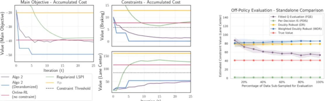
Baseline and Procedure. As a na¨ıve baseline, DDQN achieves low cost, but exhibits “non-smooth” driving behav-ior (see our supplementary videos). We set the threshold for each constraint to 75% of the DDQN benchmark. We also compare against regularized batch RL algorithms ( Farah-mand et al.,2009), specifically regularized LSPI. We in-stantiate our subroutines, FQE and FQI, with multi-layered CNNs. We augment LSPI’s linear policy with non-linear features derived from a well-performing FQI model. Results. The returned mixture policy from our algorithm achieves low main objective cost, comparable with online RL policy trained without regard to constraints. After sev-eral initial iterations violating the braking constraint, the returned policy - corresponding to the appropriateλ trade-off - satisties both constraints, while improving the main objective. The improvement over data gathering policy is significant for both constraints and main objective. Regularized policy learning is an alternative approach to (OPT) (section2). We provide the regularized LSPI base-line the same set ofλfound by our algorithm for one-shot regularized learning (Figures 2(left & middle)). While regularized LSPI obtains good performance for the main ob-jective, it does not achieve acceptable constraint satisfaction. By default, regularized policy learning requires parameter tuning heuristics. In principle, one can perform a grid-search over a range of parameters to find the right combination - we include such an example for both regularized LSPI and FQI in AppendixH. However, since our objective and constraints are in conflict, main objective and constraint satisfaction of policies returned by one-shot regularized learning are sensitive to step changes inλ. In constrast, our approach is systematic, and is able to avoid the curse-of-dimensionality of brute-force search that comes with multiple constraints. In practice, one may wish to deterministically extract a single policy from the returned mixture for execution. A de-randomized policy can be obtained naturally from our algorithm by selecting the best policy from the existing FQE’s estimates of individualBest-responsepolicies. 5.3. Off-Policy Evaluation
The off-policy evaluation by FQE is critical for updating policies in our algorithm, and is ultimately responsible for certifying constraint satisfaction. While other OPE meth-ods can also be used in place of FQE, we find that the estimates from popular methods are not sufficiently accu-rate in a high-dimensional setting. As a standalone com-parison, we select an individual policy and compare FQE against PDIS (Precup et al.,2000), DR (Jiang & Li,2016) and WDR (Thomas & Brunskill,2016) with respect to the constraint cost evaluation. To compare both accuracy and
Figure 1.FrozenLake Results.(Left)Empirical duality gap of algorithm2vs. optimal gap.(Middle)Comparison of returned policy and others w.r.t. (top) main objective value and (bottom) safety constraint value.(Right)FQE vs. other OPE methods on a standalone basis.
Figure 2.CarRacing Results.(Left)&(Middle)(Lower is better) Comparing our algorithm, regularized LSPI, online RL w/o constraints, behavior policyπDw.r.t. main cost objectives and two constraints.(Right)FQE vs. other OPE methods on a standalone basis.
data-efficiency, for each domain we randomly sample dif-ferent subsets of datasetD(from 10% to 100% transitions, 30 trials each). Figure1(right) and 2(right) illustrate the difference in quality. In the FrozenLake domain, FQE per-forms competitively with the top baseline method (DR and WDR), converging to the true value estimate as the data subsample grows close to 100%. In the high-dimensional car domain, FQE signficantly outperforms other methods.
6. Other Related Work
Constrained MDP (CMDP).The CMDP is a well-studied problem (Altman,1999). Among the most important tech-niques for solving CMDP are the Lagrangian approach and solving the dual LP program via occupation measure. How-ever, these approaches only work when the MDP is com-pletely specified, and the state dimension is small such that solving via an LP is tractable. More recently, the con-strained policy optimization approach (CPO) by (Achiam et al.,2017) learns a policy when the model is not initially known. The focus of CPO is on online safe exploration, and thus is not directly comparable to our setting.
Multi-objective Reinforcement Learning. Another related area is multi-objective reinforcement learning (MORL)(Van Moffaert & Now´e,2014;Roijers et al.,2013). Generally, research in MORL has largely focused on approx-imating the Pareto frontier that trades-off competing objec-tives (Van Moffaert & Now´e,2014;Roijers et al.,2013).
The underlying approach to MORL frequently relies on lin-ear or non-linlin-ear scalarization of rewards to heuristically turns the problem into a standard RL problem. Our pro-posed approach represents another systematic paradigm to solve MORL, whether in batch or online settings.
7. Discussion
We have presented a systematic approach for batch policy learning under multiple constraints. Our problem formula-tion can accommodate general definiformula-tion of constraints, as partly illustrated by our experiments. We provide guarantees for our algorithm for both the main objective and constraint satisfaction. Our strong empirical results show a promise of making constrained batch policy learning applicable for real-world domains, where behavior data is abundant. Our implementation complies with the steps laid out in Al-gorithm2. In very large scale or high-dimensional problems, one could consider a noisy update version for both policy learning and evaluation. We leave the theorerical and practi-cal exploration of this extension to future work. In addition, our proposed FQE algorithm for OPE problem achieves strong results, especially in a difficult domain with long horizons. Comparing the bias-variance characteristics of FQE with contemporary OPE methods is another interesting direction for research.
References
Achiam, J., Held, D., Tamar, A., and Abbeel, P. Constrained policy optimization. InInternational Conference on Machine Learning, pp. 22–31, 2017.
Agarwal, A., Beygelzimer, A., Dud´ık, M., Langford, J., and Wal-lach, H. A reductions approach to fair classification. In Interna-tional Conference on Machine Learning, 2018.
Altman, E. Constrained Markov decision processes, volume 7. CRC Press, 1999.
Antos, A., Szepesv´ari, C., and Munos, R. Fitted q-iteration in con-tinuous action-space mdps. InAdvances in neural information processing systems, pp. 9–16, 2008a.
Antos, A., Szepesv´ari, C., and Munos, R. Learning near-optimal policies with bellman-residual minimization based fitted policy iteration and a single sample path. Machine Learning, 71(1): 89–129, 2008b.
Bartlett, P. L., Harvey, N., Liaw, C., and Mehrabian, A. Nearly-tight vc-dimension bounds for piecewise linear neural networks. InProceedings of the 22nd Annual Conference on Learning Theory (COLT 2017), 2017.
Bertsekas, D. P. Approximate policy iteration: A survey and some new methods.Journal of Control Theory and Applications, 9 (3):310–335, 2011.
Blackmore, L., Ono, M., and Williams, B. C. Chance-constrained optimal path planning with obstacles. IEEE Transactions on Robotics, 27(6):1080–1094, 2011.
Bougerol, P. and Picard, N. Strict stationarity of generalized autoregressive processes.The Annals of Probability, pp. 1714– 1730, 1992.
Boyd, S. and Vandenberghe, L.Convex optimization. Cambridge university press, 2004.
Cheng, C.-A., Yan, X., Theodorou, E., and Boots, B. Accelerating imitation learning with predictive models. InConference on Artificial Intelligence and Statistics (AISTATS), 2019.
Dud´ık, M., Langford, J., and Li, L. Doubly robust policy evalu-ation and learning. InProceedings of the 28th International Conference on International Conference on Machine Learning, pp. 1097–1104. Omnipress, 2011.
Ernst, D., Geurts, P., and Wehenkel, L. Tree-based batch mode reinforcement learning.Journal of Machine Learning Research, 6(Apr):503–556, 2005.
Farahmand, A. M., Ghavamzadeh, M., Mannor, S., and Szepesv´ari, C. Regularized policy iteration. InAdvances in Neural Infor-mation Processing Systems, pp. 441–448, 2009.
Farajtabar, M., Chow, Y., and Ghavamzadeh, M. More ro-bust doubly roro-bust off-policy evaluation. arXiv preprint arXiv:1802.03493, 2018.
Freund, Y. and Schapire, R. E. Adaptive game playing using multiplicative weights. Games and Economic Behavior, 29: 79–103, 1999.
Friedman, J., Hastie, T., and Tibshirani, R.The elements of statis-tical learning. Springer, 2001.
Garcıa, J. and Fern´andez, F. A comprehensive survey on safe reinforcement learning.Journal of Machine Learning Research, 16(1):1437–1480, 2015.
Guo, Z., Thomas, P. S., and Brunskill, E. Using options and covariance testing for long horizon off-policy policy evaluation. In Advances in Neural Information Processing Systems, pp. 2492–2501, 2017.
Gy¨orfi, L., Kohler, M., Krzyzak, A., and Walk, H.A distribution-free theory of nonparametric regression. Springer Science & Business Media, 2006.
Ha, D. and Schmidhuber, J. World models. arXiv preprint arXiv:1803.10122, 2018.
Haarnoja, T., Tang, H., Abbeel, P., and Levine, S. Reinforcement learning with deep energy-based policies. In International Conference on Machine Learning, pp. 1352–1361, 2017. Haussler, D. Sphere packing numbers for subsets of the boolean
n-cube with bounded vapnik-chervonenkis dimension.Journal of Combinatorial Theory, Series A, 69(2):217–232, 1995. Henaff, M., Canziani, A., and LeCun, Y. Model-predictive policy
learning with uncertainty regularization for driving in dense traffic.arXiv preprint arXiv:1901.02705, 2019.
Hester, T., Vecerik, M., Pietquin, O., Lanctot, M., Schaul, T., Piot, B., Horgan, D., Quan, J., Sendonaris, A., Osband, I., et al. Deep q-learning from demonstrations. InThirty-Second AAAI Conference on Artificial Intelligence, 2018.
Jiang, N. and Li, L. Doubly robust off-policy value evaluation for reinforcement learning. InInternational Conference on Machine Learning, pp. 652–661, 2016.
Kakade, S. and Langford, J. Approximately optimal approximate reinforcement learning. InICML, volume 2, pp. 267–274, 2002. Kivinen, J. and Warmuth, M. K. Exponentiated gradient versus gradient descent for linear predictors.Information and Compu-tation, 132(1):1–63, 1997.
Koenig, S. and Simmons, R. G. The effect of representation and knowledge on goal-directed exploration with reinforcement-learning algorithms. Machine Learning, 22(1-3):227–250, 1996.
Lagoudakis, M. G. and Parr, R. Least-squares policy iteration.
Journal of machine learning research, 4(Dec):1107–1149, 2003. Lange, S., Gabel, T., and Riedmiller, M. Batch reinforcement
learning. InReinforcement learning, pp. 45–73. Springer, 2012. Lazaric, A. and Restelli, M. Transfer from multiple mdps. In
Advances in Neural Information Processing Systems, pp. 1746– 1754, 2011.
Lazaric, A., Ghavamzadeh, M., and Munos, R. Finite-sample analysis of lstd. InICML-27th International Conference on Machine Learning, pp. 615–622, 2010.
Lazaric, A., Ghavamzadeh, M., and Munos, R. Finite-sample analysis of least-squares policy iteration. Journal of Machine Learning Research, 13(Oct):3041–3074, 2012.
Le, H. M., Kang, A., Yue, Y., and Carr, P. Smooth imitation learning for online sequence prediction. InProceedings of the 33rd International Conference on International Conference on Machine Learning-Volume 48, pp. 680–688. JMLR. org, 2016. Lee, W. S., Bartlett, P. L., and Williamson, R. C. Efficient ag-nostic learning of neural networks with bounded fan-in.IEEE Transactions on Information Theory, 42(6):2118–2132, 1996. Levine, S. and Abbeel, P. Learning neural network policies with
guided policy search under unknown dynamics. InAdvances in Neural Information Processing Systems, pp. 1071–1079, 2014. Lillicrap, T. P., Hunt, J. J., Pritzel, A., Heess, N., Erez, T., Tassa, Y., Silver, D., and Wierstra, D. Continuous control with deep re-inforcement learning. InInternational Conference on Learning Representations (ICLR), 2016.
Liu, Q., Li, L., Tang, Z., and Zhou, D. Breaking the curse of horizon: Infinite-horizon off-policy estimation. InAdvances in Neural Information Processing Systems, pp. 5361–5371, 2018. Maillard, O.-A., Munos, R., Lazaric, A., and Ghavamzadeh, M. Finite-sample analysis of bellman residual minimization. In
Proceedings of 2nd Asian Conference on Machine Learning, pp. 299–314, 2010.
Mohri, M., Rostamizadeh, A., and Talwalkar, A.Foundations of machine learning. MIT press, 2012.
Montgomery, W. H. and Levine, S. Guided policy search via approximate mirror descent. InAdvances in Neural Information Processing Systems, pp. 4008–4016, 2016.
Munos, R. Error bounds for approximate policy iteration. InICML, volume 3, pp. 560–567, 2003.
Munos, R. Performance bounds in l p-norm for approximate value iteration. SIAM journal on control and optimization, 46(2): 541–561, 2007.
Munos, R. and Szepesv´ari, C. Finite-time bounds for fitted value iteration.Journal of Machine Learning Research, 9(May):815– 857, 2008.
Nemirovsky, A. S. and Yudin, D. B. Problem complexity and method efficiency in optimization.Wiley, 1983.
Oh, J., Guo, Y., Singh, S., and Lee, H. Self-imitation learning. In
International Conference on Machine Learning, 2018. Ono, M., Pavone, M., Kuwata, Y., and Balaram, J.
Chance-constrained dynamic programming with application to risk-aware robotic space exploration. Autonomous Robots, 39(4): 555–571, 2015.
Ormoneit, D. and Sen, ´S. Kernel-based reinforcement learning.
Machine learning, 49(2-3):161–178, 2002.
Pietquin, O., Geist, M., Chandramohan, S., and Frezza-Buet, H. Sample-efficient batch reinforcement learning for dialogue man-agement optimization.ACM Transactions on Speech and Lan-guage Processing (TSLP), 7(3):7, 2011.
Precup, D., Sutton, R. S., and Singh, S. P. Eligibility traces for off-policy policy evaluation. InProceedings of the Seventeenth International Conference on Machine Learning, pp. 759–766. Morgan Kaufmann Publishers Inc., 2000.
Precup, D., Sutton, R. S., and Dasgupta, S. Off-policy temporal dif-ference learning with function approximation. InProceedings of the Eighteenth International Conference on Machine Learning, pp. 417–424. Morgan Kaufmann Publishers Inc., 2001. Riedmiller, M. Neural fitted q iteration–first experiences with a
data efficient neural reinforcement learning method. In Euro-pean Conference on Machine Learning, pp. 317–328. Springer, 2005.
Riedmiller, M., Gabel, T., Hafner, R., and Lange, S. Reinforcement learning for robot soccer. Autonomous Robots, 27(1):55–73, 2009.
Roijers, D. M., Vamplew, P., Whiteson, S., and Dazeley, R. A survey of multi-objective sequential decision-making.Journal of Artificial Intelligence Research, 48:67–113, 2013.
Ross, S. and Bagnell, J. A. Reinforcement and imitation learning via interactive no-regret learning. arXiv preprint arXiv:1406.5979, 2014.
Schulman, J., Levine, S., Abbeel, P., Jordan, M., and Moritz, P. Trust region policy optimization. InInternational Conference on Machine Learning, pp. 1889–1897, 2015.
Shalev-Shwartz, S. et al. Online learning and online convex opti-mization. Foundations and TrendsR in Machine Learning, 4 (2):107–194, 2012.
Sutton, R. S. and Barto, A. G.Reinforcement learning: An intro-duction. MIT press, 2018.
Swaminathan, A. and Joachims, T. Batch learning from logged bandit feedback through counterfactual risk minimization. Jour-nal of Machine Learning Research, 16(1):1731–1755, 2015. Thomas, P. and Brunskill, E. Data-efficient off-policy policy
eval-uation for reinforcement learning. InInternational Conference on Machine Learning, pp. 2139–2148, 2016.
Van Hasselt, H., Guez, A., and Silver, D. Deep reinforcement learning with double q-learning. InAAAI, volume 2, pp. 5. Phoenix, AZ, 2016.
Van Moffaert, K. and Now´e, A. Multi-objective reinforcement learning using sets of pareto dominating policies.The Journal of Machine Learning Research, 15(1):3483–3512, 2014. Von Neumann, J. and Morgenstern, O.Theory of games and
eco-nomic behavior (commemorative edition). Princeton university press, 2007.
Wang, Y.-X., Agarwal, A., and Dud´ık, M. Optimal and adaptive off-policy evaluation in contextual bandits. InInternational Conference on Machine Learning, pp. 3589–3597, 2017. Ziebart, B. D. Modeling purposeful adaptive behavior with the
principle of maximum causal entropy. PhD thesis, CMU, 2010. Ziebart, B. D., Maas, A. L., Bagnell, J. A., and Dey, A. K. Max-imum entropy inverse reinforcement learning. InAAAI, vol-ume 8, pp. 1433–1438. Chicago, IL, USA, 2008.
Zinkevich, M. Online convex programming and generalized in-finitesimal gradient ascent. InProceedings of the 20th Interna-tional Conference on Machine Learning (ICML-03), pp. 928– 936, 2003.
A. Equivalence between Regularization and Constraint Satisfaction
A.1. Formulating Different Regularized Policy Learning Problems as Constrained Policy Learning
In this section, we provide connections between regularized policy learning and our constrained formulation (OPT). Although the main paper focuses on batch policy learning, here we are agnostic between online and batch learning settings. Entropy regularized RL. The standard reinforcement learning objective, either in online or batch setting, is to find a policy π∗std that minimizes the long-term cost (equivalent to maximizing the accumuted rewards): πstd∗ = arg minπP
tE(xt,at)∼π[c(xt, at)] = arg minπE(x,a)∼µπ[c(x, a)]. Maximum entropy reinforcement learning (Haarnoja
et al.,2017) augments the cost with an entropy term, such that the optimal policy maximizes its entropy at each visited state: πMaxEnt∗ = arg minπE(x,a)∼µπ[c(x, a)]−λH(π(·|x)). As discuseed by (Haarnoja et al.,2017), the goal is for the
agent to maximize the entropy of the entire trajectory, and not greedily maximizing entropy at the current time step (i.e., Boltzmann exploration). Maximum entropy policy learning was first proposed by (Ziebart et al.,2008;Ziebart,2010) in the context of learning from expert demonstrations. Entropy regulazed RL/IL is equivalent to our problem (OPT) by simply set
C(π) =E(xt,at)∼π[c(xt, at)](standard RL objective), andg(x, a) =π(a|x) logπ(a|x), thusG(π) =−H(π)≤τ
Smooth imitation learning (& Regularized imitation learning).This is a constrained imitation learning problem studied by (Le et al.,2016): learning to mimic smooth behavior in continuous space from human desmonstrations. The data collected from human demonstrations is considered to be fixed and given a priori, thus the imitation learning task is also a batch policy learning problem. The proposed approach from (Le et al.,2016) is to view policy learning as a function regularization problem: policyπ= (f, g)is a combination of functionsf andh, wheref belongs to some expressive function classF
(e.g., decision trees, neural networks) andh∈Hwith certifiable smoothness property (e.g., linear models). Policy learning is the solution to the functional regularization problem π = arg minf,gEx∼µπkf(x)−πE(x)k+λkh(x)−πE(x)k,
whereπEis the expert policy. This constrained imitation learning setting is equivalent to our problem (OPT) as follows:
C(π) =C((f, h)) =Ex∼µπkf(x)−πE(x)kandG(π) =G((f, h)) = minh0∈Hkh
0(x)−π
E(x)k ≤τ
Regularizing RL with expert demonstrations / Learning from imperfect demonstrations.Efficient exploration in RL is a well-known challenge. Expert demonstrations provide a way around online exploration to reduce the sample complexity for learning. However, the label budget for expert demonstrations may be limited, resulting in a sparse coverage of the state space compared to what the online RL agent can explore (Hester et al.,2018). Additionally, expert demonstrations may be imperfect (Oh et al.,2018). Some recent work proposed to regularize standard RL objective with some deviation measure between the learning policy and (sparse) expert data (Hester et al.,2018;Oh et al.,2018;Henaff et al.,2019).
For clarity we focus on the regularized RL objective for Q-learning in (Hester et al.,2018), which is defined asJ(π) =
JDQ(Q)+λ1Jn(Q)+λ2JE(Q)+λ3JL2(Q), whereJDQ(Q)is the standard deep Q-learning loss,Jn(Q)is the n-step return loss,JE(Q)is the imitation learning loss defined asJE(Q) = maxa∈A[Q(x, a) +`(aE, a)−Q(x, aE)], andJL2(Q)is an L2 regularization loss applied to the Q-network to prevent overfitting to a small expert dataset. The regularization parameters
λ’s are obtained by hyperparameter tuning. This approach provides a bridge between RL and IL, whose objective functions are fundamentally different (see AggreVate by (Ross & Bagnell,2014) for an alternative approach).
We can cast this problem into (OPT) as: C(π) = CDQ(Q) +λ3CL2(Q)(standard RL objective), and two constraints:
g1(π) = Ex∼µπ[maxa∈AQ(x, a) +`(aE, a)−Q(x, aE)], and g2(x, a) = Ex∼µπ[ct+γct+1 +. . .+γ
n−1c
t+n−1+
min0aγnQ(xt+n, a0)−Q(xt, a)]. Hereg1captures the loss w.r.t. expert demonstrations andg2reflects the n-step return constraint.
More generally, one can define the imitation learning constraint asG(π) = Ex∼µπ`(π(x), πE(x))for an appropriate
divergence definition betweenπ(x)andπE(x)(defined at states where expert demonstrations are available).
Conservative policy improvement.Many policy search algorithms perform small policy update steps, requiring the new policyπto stay within a neighborhood of the most recent policy iterateπkto ensure learning stability (Levine & Abbeel,
2014;Schulman et al.,2015;Montgomery & Levine,2016;Achiam et al.,2017). This simply corresponds to the definition ofG(π) =distance(π, πk)≤τ, wheredistanceis typicallyKL-divergence or total variation distance between the distribution induced byπandπk. ForKL-divergence, the single timestep costg(x, a) =−π(a|x) log(
πk(a|x)
A.2. Equivalence of Regularization and Constraint Viewpoint - Proof of Proposition2.1
Regularization=⇒Constraint: Letλ >0andπ∗be optimal policy inRegularization. Setτ =G(π∗). Suppose thatπ∗is not optimal inConstraint. Then∃π∈Πsuch thatG(π)≤τandC(π)< C(π∗). We then have
C(π) +λ>G(π)< C(π∗) +λ>τ=C(π∗) +λ>G(π∗)
which contradicts the optimality ofπ∗ forRegularizationproblem. Thusπ∗ is also the optimal solution of the
Constraintproblem.
Constraint=⇒Regularization: Givenτand letπ∗be the corresponding optimal solution of theConstraint
problem. The Lagrangian of Constraint is given byL(π, λ) = C(π) +λ>G(π), λ ≥ 0. We then have π∗ = arg min π∈Π max λ≥0L(π, λ). Let λ∗= arg max λ≥0 min π∈ΠL(π, λ)
Slater’s condition implies strong duality. By strong duality and the strong max-min property (Boyd & Vandenberghe,2004), we can exchange the order of maximization and minimization. Thusπ∗is the optimal solution of
min
π∈Π C(π) + (λ
∗)>(G(π)−τ)
Removing the constaint(λ∗)>τ, we have thatπ∗is the optimal solution of theRegularizationproblem withλ=λ∗. And sinceπ∗6= arg min
π∈Π
B. Convergence Proofs
B.1. Convergence of Meta-algorithm - Proof of Proposition3.1
Let us evaluate the empirical primal-dual gap of the Lagrangian afterTiterations:
max λ L(πbT, λ) = maxλ 1 T X t L(πt, λ) (1) ≤ 1 T X t L(πt, λt) + o(T) T (2) ≤ 1 T X t L(π, λt) + o(T) T ∀π∈Π (3) =L(π,bλT) + o(T) T ∀π (4)
Equations (1) and (4) are due to the definition ofbπT andλbT and linearity ofL(π, λ)wrtλand the distribution over policies inΠ. Equation (2) is due to the no-regret property ofOnline-algorithm. Equation (3) is true sinceπtis best response wrtλt. Since equation (4) holds for allπ, we can conclude that forT sufficiently large such that o(TT) ≤ ω, we have
maxλL(πbT, λ)≤minπL(π,λbT) +ω, which will terminate the algorithm.
Note that we always havemaxλL(bπT, λ)≥L(bπT,λbT)≥minπL(π,λbT). Algorithm1’s convergence rate depends on the regret bound of theOnline-algorithmprocedure. Multiple algorithms exist with regret scaling asΩ(√T)(e.g., online gradient descent with regularizer, variants of online mirror descent). In that case, the algorithm will terminate afterO(ω12)
iterations.
B.2. Empirical Convergence Analysis of Main Algorithm - Proof of Theorem4.1
By choosing normalized exponentiated gradient as the online learning subroutine, we have the following regret bound after
T iterations of the main algorithm2(chapter 2 of (Shalev-Shwartz et al.,2012)) for anyλ∈R+m+1,kλk1=B:
1 T T X t=1 b L(πt, λ)≤ 1 T T X t=1 b L(πt, λt) + Blog(m+1) η +ηG 2BT T (5) DenoteωT = Blog(m+1) η +ηG 2BT
T to simplify notations. By the linearity ofLb(π, λ)in bothπandλ, we have for anyλthat b L(bπT, λ) linearity = 1 T T X t=1 b L(πt, λ) eqn(5) ≤ 1 T T X t=1 b L(πt, λt) +ωT best responseπt ≤ 1 T T X t=1 b L(πbT, λt) +ωT linearity = Lb(bπT,λbT) +ωT Since this is true for anyλ,maxλLb(bπT, λ)≤Lb(bπT,bλT) +ωT.
On the other hand, for any policyπ, we also have
b L(π,bλT) linearity = 1 T T X t=1 b L(π, λt) best responseπt ≥ 1 T T X t=1 b L(πt, λt) eqn(5) ≥ 1 T T X t=1 b L(πt,bλT)−ωT linearity = Lb(bπT,bλT)−ωT ThusminπLb(π,bλT)≥Lb(πbT,bλT)−ωT, leading to
max
λ Lb(πbT, λ)−minπ Lb(π,bλT)≤Lb(πbT,bλT) +ωT−(Lb(πbT,bλT)−ωT) = 2ωT AfterTiterations of the main algorithm2, therefore, the empirical primal-dual gap is bounded by
max
λ Lb(bπT, λ)−minπ Lb(π,bλT)≤
2Blog(ηm+1)+ 2ηG2BT
T
In particular, if we want the gap to fall below a desired thresholdω, setting the online learning rateη= ω
4G2B will ensure
C. End-to-end Generalization Analysis of Main Algorithm
In this section, we prove the following full statement of theorem4.4of the main paper. Note that to lessen notation, we defineV =C+BGto be the bound of value functions under considerations in algorithm2.
Theorem C.1(Generalization bound of algorithm2). Letπ∗be the optimal policy to problemOPT. LetKbe the number of iterations of FQE and FQI. Letπbbe the policy returned by our main algorithm2, with termination thresholdω. For any
>0, δ∈(0,1), whenn≥ 24·214·V4 2 log K(m+1) δ +dimFlog 320V2 2 + log(14e(dimF+ 1))
, we have with probability at least1−δ: C(bπ)≤C(π∗) +ω+(4 +B)γ (1−γ)3 p Cρ+ 2γK/2V and G(πb)≤τ+ 2V +ω B + γ1/2 (1−γ)3/2 p Cρ+ 2γK/2V (1−γ)1/2 Letbπ= 1 T P
tπtbe the returned policyTiterations, with corresponding dual variablebλ=T1Ptλt. By the stopping condition, the empirical duality gap is less than some threshold ω, i.e., max
λ∈Rm++1,kλk1=B b L(π, λb )− min π∈ΠLb(π,bλ) ≤ ω where Lb(π, λ) = Cb(π) +λ >( b
G(π)−τ). We first show that the returned policy approximately satisfies the constraints. The proof of theoremC.1will make use of the following empirical constraint satisfaction bound: Lemma C.2(Empirical constraint satisfactions). Assume that the constraintsGb(π)≤τ are feasible. Then the returned policyπbapproximately satisfies all constraints
max
i=1:m+1(gbi(πb)−τi)≤2
C+ω B
Proof. We consider max
i=1:m+1(bgi(bπ)−τi)>0(otherwise the lemma statement is trivially true). The termination condition implies thatLb(bπ,bλ)− max
λ∈Rm++1,kλk1=B b L(bπ, λ)≥ −ω =⇒ bλ>(Gb(bπ)−τb)≥ max λ∈Rm++1,kλk1=B λ>(Gb(bπ)−bτ)−ω (6)
Relaxing the RHS of equation (6) by settingλ[j] =Bforj = arg max
i=1:m+1 [bgi(πb)−τi]andλ[i] = 0 ∀i6=jyields: B max i=1:m+1[gbi(πb)−τi]−ω≤bλ >( b G(πb)−τ) (7)
Givenπsuch thatGb(π)≤τ, also by the termination condition: b L(bπ,λb)−Lb(π,bλ)≤ max λ∈Rm++1,kλk1=B b L(bπ, λ)−min π∈ΠLb(π,bλ)≤ω Thus implies b L(π,b bλ)≤Lb(π,bλ) +ω=Cb(π) +bλ>(Gb(π)−τ)≤Cb(π) +ω (8) combining what we have from equation (8) and (7):
B max
i=1:m+1[gbi(πb)−bτi]−ω≤bλ >(
b
G(πb)−bτ) =Lb(π,b bλ)−Cb(bπ)≤Cb(π) +ω−Cb(bπ) Rearranging and boundingCb(π)≤CandCb(bπ)≤ −Cfinishes the proof of the lemma.
We now return to the proof of theoremC.1, our task is to lift empirical error to generalization bound for main objective and constraints.
Denote byF QEthe (generalization) error introduced by the Fitted Q Evaluation procedure (algorithm3) andF QI the (generalization) error introduced by the Fitted Q Iteration procedure (algorithm4). For now we keepF QE andF QI unspecified (to be specified shortly). That is, for eacht= 1,2, . . . , T, we have with probability at least1−δ:
Sinceπ∗satisfies the constraints, i.e.,G(π∗)−τ ≤0componentwise, andλt≥0, we also have with probability1−δ
L(πt, λt) =C(πt) +λ>t(G(πt)−τ)≤C(π∗) +F QI (9) Similarly, with probability1−δ, all of the following inequalities are true
b
C(πt) +F QE≥C(πt)≥Cb(πt)−F QE (10)
b
G(πt) +F QE1≥G(πt)≥Gb(πt)−F QE1(row wise for allmconstraints) (11) Thus with probability at least1−δ
L(πt, λt) =C(πt) +λ>t(G(πt)−τ)≥Cb(πt) +λ>t(Gb(πt)−τ)−F QE(1 +λ>t1) ≥Cb(πt) +λ>t(Gb(πt)−τ)−F QE(1 +B)
=Lb(πt, λt)−F QE(1 +B) (12) Recall that the execution of mixture policybπis done by uniformly sampling one policyπtfrom{π1, . . . , πT}, and rolling-out withπt. Thus from equations (9) and (12), we haveEt∼U[1:T]Lb(πt, λt)≤C(π∗) +F QI+ (1 +B)F QE w.p.1−δ. In other words, with probability1−δ:
1 T T X t=1 b L(πt, λt)≤C(π∗) +F QI+ (1 +B)F QE Due to the no-regret property of our online algorithm (EG in this case):
1 T T X t=1 b L(πt, λt)≥max λ Lb(bπ, λ)−ω=Cb(bπ) + maxλ λ >( b G(πb)−τ)−ω
IfGb(bπ)−τ≤0componentwise, chooseλ[i] = 0, i= 1,2, . . . , mandλ[m+ 1] =B. Otherwise, we can chooseλ[j] =B forj= arg max
i=1:m+1
[bgi(bπ)−τ[i]]andλ[i] = 0 ∀i6=j. We can see that max λ∈Rm++1,kλk1=B
λ>(Gb(πb)−τ)≥0. Therefore:
b
C(πb)−ω≤C(π∗) +F QI+ (1 +B)F QEwith probability at least1−δ Combined with the first term from equation (10):
C(bπ)−F QE−ω≤C(π∗) +F QI+ (1 +B)F QE or
C(πb)≤C(π∗) +ω+F QI+ (2 +B)F QE (13) We now bring in the generalization error results from our standalone analysis of FQI (appendixF) and FQE (appendixE) into equation (13).
Specifically, whenn≥ 24·214·V4 2
logK(mδ+1)+dimFlog320V
2
2 + log(14e(dimF+ 1))
, when FQI and FQE are run withKiterations, we have the guarantee that for any >0, with probability at least1−δ
C(bπ)≤C(π∗) +ω+ 2γ (1−γ)3 p Cµ+ 2γK/2V | {z }
FQI generalization error
+γ 1/2(2 +B) (1−γ)3/2 p Cµ+ γK/2 (1−γ)1/22V | {z }
(2+B)×FQE generalization error ≤C(π∗) +ω+(4 +B)γ (1−γ)3 p Cµ+ 2γK/2V (14) From lemma C.2, Gb(bπ) ≤ τ + 2C+Bω ≤ τ + 2VB+ω. From equation (11), for each t=1,2,. . . ,T, we have Gb(πt) ≥
G(πt)−F QE1with probability1−δ. Thus
PGb(bπ)≥G(bπ)−F QE1 = T X t=1 P(Gb(πt)≥G(πt)−F QE1|bπ=πt)P(πb=πt)≥T(1−δ) 1 T = 1−δ
Therefore, we have the following generalization guarantee for the approximate satisfaction of all constraints:
G(bπ)≤τ+ 2V +ω B + γ1/2 (1−γ)3/2 p Cµ+ γK/2 (1−γ)1/22V (15) Inequalities (14) and (15) complete the proof of theoremC.1(and theorem4.4of the main paper)
D. Preliminaries to Analysis of Fitted Q Evaluation (FQE) and Fitted Q Iteration (FQI)
In this section, we set-up necessary notations and definitions for the theoretical analysis of FQE and FQI. To simplify the presentation, we will focus exclusively on weighted`2norm for error analysis.
With the definitions and assumptions presented in this section, we will present the sample complexity guarantee of Fitted-Q-Evaluation (FQE) in appendixE. The proof for FQI will follow similarly in appendixF.
While it is possible to adapt proofs from related algorithms (Munos & Szepesv´ari,2008;Antos et al.,2008b) to analyze FQE and FQI, in the next two sections we show improved convergence rate fromO(n−4)toO(n−2), wherenis the number of samples in data setD.
To be consistent with the notations in the main paper, we use the conventionC(π)as the value function that denotes long-term accumulated cost, instead of usingV(π)denoting long-term rewards in the traditional RL literature. Our notation forQfunction is similar to the RL literature - the only difference is that the optimal policy minimizesQ(x, a)instead of maximizing. We denote the bound on the value function asC(alternatively if the single timestep cost is bounded byc, then
C= c
1−γ). For simplicity, the standalone analysis of FQE and FQI concerns only with the cost objectivec. Dealing with costc+λ>goffers no extra difficulty - in that case we simply augment the bound of the value function toV =C+BG. D.1. Bellman operators
TheBellman optimality operatorT:B(X×A;C)7→ B(X×A;C)as
(TQ)(x, a) =c(x, a) +γ Z X min a0∈AQ(x 0, a0)p(dx0|x, a) (16) The optimal value functions are defined as usual byC∗(x) = sup
π
Cπ(x)andQ∗(x, a) = sup
π
Qπ(x, a) ∀x∈X, a∈A. For a given policyπ, theBellman evaluation operatorTπ:B(X×A;C)7→ B(X×A;C)as
(TπQ)(x, a) =c(x, a) +γ Z
X
Q(x0, π(x0))p(dx0|x, a) (17) It is well known thatTπQπ =Qπ,a fixed point of theTπoperator.
D.2. Data distribution and weighted`2norm
Denote the state-action data generating distribution asµ, induced by some data-generating (behavior) policyπD, that is,
(xi, ai)∼µfor(xi, ai, x0i, ci)∈D.
Note that data set Dis formed by multiple trajectories generated byπD. For each(xi, ai), we havex0i ∼ p(·|xi, ai) andci = c(xi, ai). For any (measurable) functionf : X×A 7→ R, define theµ-weighted`2 norm off askfk2µ = R
X×Af(x, a)
2µ(dx, da) = R
X×Af(x, a) 2µ
x(dx)πD(a|dx). Similarly for any other state-action distributionρ,kfk 2 ρ = R
X×Af(x, a)
2ρ(dx, da) D.3. Inherent Bellman error
FQE and FQI depend on a chosen function classFto approximateQ(x, a). To express how well the Bellman operatorTg
can be approximated by a function in the policy classF, whenTg /∈F, a notion of distance, known as inherent Bellman error was first proposed by (Munos,2003) and used in the analysis of related ADP algorithms (Munos & Szepesv´ari,2008;
Munos,2007;Antos et al.,2008a;b;Lazaric et al.,2010;2012;Lazaric & Restelli,2011;Maillard et al.,2010).
Definition D.1(Inherent Bellman Error). Given a function classFand a chosen distributionρ, theinherent Bellman error ofFis defined as
dF=d(F,TF) = sup h∈F
inf
f∈Fkf −Thkρ
wherek·kρis theρ−weighted`2norm andTis the Bellman optimality operator defined in (16) To analyze FQE, we will form a similar definition for the Bellman evaluation operator
evaluation errorofFis defined as dπF=d(F,TπF) = sup h∈F inf f∈Fkf−T πhk ρπ wherek·kρ
πis the`2norm weighted byρπ.ρπis defined as the state-action distribution induced by policyπ, andT
πis the Bellman operator defined in (17)
D.4. Concentration coefficients
LetPπdenote the operator acting onf : X×A7→
Rsuch that(Pπf)(x, a) =RXf(x
0, π(x0))p(x0|x, a)dx0. Acting onf (e.g., approximatesQ),Pπcaptures the transition dynamics of taking actionaand followingπthereafters.
The following definition and assumption are standard in the analysis of related approximate dynamic programming algorithms (Lazaric et al.,2012;Munos & Szepesv´ari,2008;Antos et al.,2008a). As approximate value iteration and policy iteration algorithms perform policy update, the new policy at each round will induce a different stationary state-action distribution. One way to quantify the distribution shift is the notion of concentrability coefficient of future state-action distribution, a variant of the notion introduced by (Munos,2003).
Definition D.3(Concentration coefficient of state-action distribution). Given data generating distributionµ∼πD, initial state distributionχ. Form≥0, and an arbitrary sequence of stationary policies{πm}m≥1let
βµ(m) = sup π1,...,πm d(χPπ1Pπ2. . . Pπm) dµ ∞
(βµ(m) = ∞ if the future state distribution χPπ1Pπ2. . . Pπm is not absolutely continuous w.r.t. µ, i.e,
χPπ1Pπ2. . . Pπm(x, a)>0for someµ(x, a) = 0)
Assumption 3. βµ= (1−γ)2 P m≥1
mγm−1β
µ(m)<∞
Combination Lock Example. An example of an MDP that violates Assumption3is the “combination lock” example proposed by (Koenig & Simmons,1996). In this finite MDP, we haveNstatesX ={1,2, . . . , N}, and 2 actions: going L or R. The initial state isx0= 1. In any statex, actionLtakes agent back to initial statex0, and actionRadvances the agent to the next statex+ 1in a chain fashion. Suppose that the reward is 0 everywhere except for the very last stateN. One can see that for an MDP such that any behavior policyπDthat has a bounded from below probability of taking actionLfrom any statex, i.e.,πD(L|x)≥ν >0, then it takes an exponential number of trajectories to learn or evaluate a policy that always takes actionR. In this setting, we can see that the concentration coefficientβµcan be designed to be arbitrarily large.
D.5. Complexity measure of function classF
Definition D.4(RandomL1Norm Covers). Let >0, letFbe a set of functionsX7→R, letxn1 = (x1, . . . , xn)benfixed points inX. Then a collection of functionsF={f1, . . . , fN}is an-cover ofFonxn1 if
∀f ∈F,∃f0 ∈F:| 1 n n X i=1 f(xi)− 1 n n X i=1 f0(xi)| ≤ The empirical covering number, denote byN1(,F, xn
1), is the size of the smallest-cover onxn1. TakeN1(,F, xn1) =∞ if no finite-cover exists.
Definition D.5 (Pseudo-Dimension). A real-valued function classFhas pseudo-dimensiondimF defined as the VC dimension of the function class induced by the sub-level set of functions ofF. In other words, define function class
H ={(x, y)7→sign(f(x)−y:f ∈F}, then