Dynamic Capacity Acquisition and
Assignment under Uncertainty
∗
Shabbir Ahmed
†and Renan Garcia
School of Industrial & Systems Engineering
Georgia Institute of Technology
Atlanta, GA 30332.
March 29, 2002
Abstract
Given a set ofmresources andntasks, the dynamic capacity acquisi-tion and assignment problem seeks a minimum cost schedule of capacity acquisitions for the resources and the assignment of resources to tasks, over a given planning horizon of T periods. This problem arises, for example, in the integrated planning of locations and capacities of distri-bution centers (DCs), and the assignment of customers to the DCs, in supply chain applications. We consider the dynamic capacity acquisition and assignment problem in an environment where the assignment costs and the processing requirements for the tasks are uncertain. Using a sce-nario based approach, we develop a stochastic integer programming model for this problem. The highly non-convex nature of this model prevents the application of standard stochastic programming decomposition algo-rithms. We use a recently developed decomposition based branch-and-bound strategy for the problem. Encouraging preliminary computational results are provided.
Keywords: Capacity expansion, Stochastic integer programming, Decom-position, Branch & bound.
∗This research has been supported in part by the National Science Foundation (Grant No.
DMI-0099726) and The Logistics Institute Asia-Pacific in Singapore.
1
Introduction
We address the problem of determining a capacity expansion schedule for a set of resources, and the assignment of resource capacity to tasks over a multi-period planning horizon. This problem commonly arises in the integrated planning of locations and capacities of distribution centers (DCs), and the assignment of customers to the DCs, in supply chain applications, as well as machine pro-curement planning in manufacturing applications. In this paper, we address the problem in an uncertain setting. We develop a model that explicitly incor-porates uncertainty in task processing requirements and costs via a set of sce-narios. The resulting formulation is a stochastic integer program. The highly non-convex nature of this model prevents the application of standard stochastic programming decomposition algorithms. We describe a decomposition based branch-and-bound strategy to solve the problem to global optimality. Our pre-liminary computational experience demonstrates that the proposed algorithm significantly outperforms straight-forward use of commercial solvers, and that the method is quite insensitive to the number of scenarios.
The remainder of the paper is organized as follows. Section 2 presents a mathematical statement of the problem under consideration. Section 3 iden-tifies some of the computational challenges in solving this class of problems. Section 4 describes a decomposition based branch and bound algorithm for the problem under consideration. Section 5 reports our preliminary computational experience using the proposed methodology. Finally, some concluding remarks are provided in Section 6.
2
Model Development
In this section, we develop a mathematical model for dynamic capacity acquisi-tion and assignment under uncertainty. We first describe a deterministic formu-lation, and later extend this formulation to a stochastic setting by introducing a set of scenarios.
2.1
The Deterministic Problem
Consider the problem of deciding the capacity expansion schedule for a setm
resources overT time periods in order to satisfy the processing requirements of n tasks. Using variables xit for the capacity acquisition of resource i in
periodt, andyijt to indicate whether resourceiis assigned to taskj in period
t, the combined capacity acquisition and assigned problem can be formulated as follows:
min Tt=1mi=1fit(xit) + m i=1 n j=1cijtyijt s.t. x∈X ⊆RmT + n j=1djtyijt ≤ τ≤txiτ ∀i, t m i=1yijt= 1 ∀j, t yijt∈ {0,1} ∀i, j, t. (1)
In the above formulationfit(·) is the expansion cost for resourceiin periodt, and
cijt is the cost of assigning resource ito taskj in periodt. The setX denotes
the constraints on capacity acquisition. The parameter djt is the processing
requirement of task j in period t, and accordingly, the second constraint in problem (1) reflects that the processing requirement of all tasks assigned to a resource in any period cannot exceed the installed capacity in that period. The third constraint enforces that each task needs to be assigned to exactly once resource in each of the periods. The final constraint enforces the binary restrictions on the assignment variablesyijt.
Typically the capacity expansion costs are modeled as fixed-charge cost func-tions, i.e. fit(xit) :=αitxit+βituit, with uit= 1 if xit>0 0 otherwise,
where αit and βit are the variable and fixed cost, respectively, of capacity
ac-quisition of resourcei in periodt, anduit is the indicator variable for capacity
acquisition. Furthermore, the setXtypically represents polyhedral constraints. In this setting, if the problem parameters, such as processing requirements and costs, are known with complete certainty, problem (1) is a deterministic mixed-integer linear program.
Various authors have considered the deterministic problem (1) in the con-text of integrated facility location and capacity planning. The resources can be viewed as potential locations for facilities, and the tasks can be interpreted as customers that need to be assigned to facilities. The integrated facility location and capacity planning problem then consists of determining where to locate fa-cilities, how much capacity to install in the various locations, and how to assign customers to facilities over a multi-period planning horizon. Fong and Srini-vasan [9, 10] considered a multi-period location and capacity planning model, and proposed a heuristic solution strategy. Their model assumed that a fraction of a customers demand could be satisfied from a facility rather than assigning all of a customer’s demand to a facility as in our problem (1). Klincewicz et al. [14] proposed an iterative heuristic procedure for solving the dynamic loca-tion and capacity planning problem in the case where fracloca-tional assignment of customer demands are not allowed. More recently, Lim and Kim [16] proposed a Lagrangian relaxation based branch and bound strategy for the exact solution of this problem.
2.2
The Stochastic Problem
In practice, the problem parameters associated with the dynamic capacity ac-quisition and assignment problem (1) are rarely known with complete certainty. To incorporate uncertainty in the decision making process, we adopt a two-stage stochastic programming approach [3]. We assume that the capacity planning decisions (for the entire planning horizon) have to made here and now, with only some knowledge of future scenarios of task processing requirements and the processing costs. Once the capacities are decided, time unfolds and a cer-tain scenario of the problem parameters realizes, and then the optimal decision regarding the task-resource assignment is made. The overall objective is to de-termine a capacity acquisition plan, such that the sum of acquisition cost and the expected assignment costs is minimized. Note that although the problem is a multi-period one, since the capacity planning decisions for all periods are made in period one, the problem is essentially a two-stage one. This is often justified, since the capacity planning decisions are strategic in nature and need to be decided over longer planning periods, while the assignment decisions are more at the operational level and can be decided when more information be-comes available. In principle, the model can be improved by considering the capacity decisions to be revised as time progresses and more information be-comes available. However, such a model would result in a multi-stage stochastic integer program which is almost impossible to solve with current computational technology. Furthermore, the two-stage model often can serve as a good enough approximation to the multi-stage problem.
To incorporate the uncertainty in the processing requirements and costs, let us assume that these parameters can be realized (jointly) as one ofS scenarios. We denote the processing requirement for taskj in period t under scenarios
by ds
jt, and the cost of processing task j using resource i in period t, under
scenario s by csijt. The probability of scenario will be denoted by ps. Using these notation, we can extend the deterministic problem (1) to the following two-stage stochastic program.
min Tt=1mi=1fit(xit) + S s=1p sT t=1Q s t(x) s.t. x∈X⊆RmT+ (2) where for allt ands,
Qs t(x) := min m i=0 n j=1csijtyij s.t. nj=1ds jtyij ≤ t τ=1xiτ ∀i m i=0yij = 1 ∀j yij∈ {0,1} ∀i, j (3)
Problem (2) represents the first-stage capacity planning problem where the ob-jective is to minimize the sum of acquisition costs and expected assignment costs. The functionQs
t(x) given by (3) represents the optimal assignment cost
in period t under scenario s for a given capacity expansion schedule x. Note that we have included a dummy resource i= 0 with infinite capacity, so that
the functionQs
t is well-defined for anyx. The costcs0jt denotes the penalty of
failing to assign a resource to taskj. The dummy resource enforces the com-plete recourseproperty [3], which guarantees that there is a feasible second-stage assignment in all periods and all scenarios for any capacity acquisition schedule. Several authors have addressed the stochastic dynamic capacity acquisition and allocation problem which allows fractions of the processing requirement of a task to be assigned to a resource. In this case the capacity allocation problem (3) in the second stage is a linear program. Such problems have been considered in the context of service industries [2], process industries [17], and the semiconductor industries [24], only to name a few. The fact that fractional allocations are not allowed makes our problem (2) exceedingly difficult. To our knowledge, the stochastic dynamic capacity acquisition and assignment problem (2) has not been previously addressed in the literature.
3
Computational Challenges
By introducing the assignment variablesyij for each period and scenario, the
stochastic dynamic capacity acquisition and assignment problem can be re-written as the following deterministic equivalent problem.
min Tt=1mi=1fit(xit) + S s=1 T t=1 m i=0 n j=1p scs ijtyijts s.t. x∈X ⊆RmT + n j=1d s jty s ijt≤ t τ=1xiτ ∀i, t, s m i=0y s ijt= 1 ∀j, t, s ys ijt∈ {0,1} ∀i, j, t, s (4)
For fixed charge cost functions fit, problem (4) is a large-scale mixed-integer
linear program which can, in principle, be solved using standard integer pro-gramming methodology. However, for problems when the number of scenarios
S is large, such an approach is doomed to failure since no advantage of the special problem structure is exploited. We demonstrate this computationally in Section 5.
Note that the stochastic dynamic capacity acquisition and assignment prob-lem (2) has a nice decomposable structure, wherein if the first-stage capacity decisions are fixed, the second-stage assignment decisions can be determined independently for each scenario. This is a general property for stochastic pro-gramming problems. For stochastic linear programs, i.e. when the second-stage problem is linear, the convexity of the second-second-stage value function along with this decomposability property has been exploited to develop a number of decomposition-based algorithms [4, 11, 13, 19, 25] as well as gradient-based algorithms [8, 23].
Unfortunately, our problem involves integer decisions in the second-stage and is a stochastic integer program. The main difficulty in solving stochastic integer programs is that the second-stage value function is not necessarily con-vex but only lower semicontinuous (l.s.c.). Thus, the standard decomposition
approaches that work nicely for stochastic linear programs, break down when second stage integer variables are present. Laporte and Louveaux [15] devel-oped a branch and bound scheme for stochastic integer programs with binary first stage variables. This restriction allows for the construction of optimality cuts that approximate the non-convex objective function at all binary solutions. Caroe and Tind [7] proposed to use non-linear dual functions within a Ben-ders decomposition based branch and bound framework. Branch and bound schemes are suggested for solving the resulting non-convex master problem. For continuous distribution of the problem parameters, Norkinet al.[18] developed a branch and bound algorithm that makes use of stochastic upper and lower bounds and proved almost sure convergence. Caroe [6] developed a branch and bound scheme where a Lagrangian relaxation is used as the lower bounding problem. In all of these branch and bound approaches, finite termination of the algorithm is not guaranteed unless the first stage variables,i.e., the search space, is purely discrete. As such these methods are not applicable to the stochastic dynamic capacity acquisition and assignment problem 2, since our first-stage variables are mixed-integer. Recently, Schultz et al. [22] proposed a finite algorithm for problems when the second stage is purely integer. The authors observe that, in this case, only integer values of the right hand side pa-rameters of the second stage problem are relevant. This fact is used to identify a countable set in the space of the first stage variables containing the optimal solution. Schultz et al. propose complete enumeration of this countable lat-tice to search for the optimal solution. This scheme only allows for the right hand side parameters to be uncertain. Furthermore, enumeration of a lattice point requires the solution of many small integer programming problems. Thus, explicit enumeration of all lattice points is, in general, computationally pro-hibitive. Recently, Ahmed et al. [1] developed an efficient decomposition based branch and bound algorithm for general two-stage stochastic integer programs with mixed-integer first-stage variables and pure integer second-stage variables. Unlike existing algorithms, this method avoids complete enumeration and is guaranteed to terminate finitely.
In the next section, we describe a decomposition based branch and bound al-gorithm for the stochastic dynamic capacity acquisition and assignment problem based upon the scheme of [1].
4
A Decomposition based Branch & Bound
Al-gorithm
Problem (2) is a two-stage stochastic integer program with mixed-integer first-stage variables, and pure integer second-first-stage variables. Since we have assumed that dummy resourcesy0j have been introduced for eachj, the problem
obvi-ously possesses thecomplete recourse property, i.e., Qst(x)<∞ for all x∈ X
and for allt ands. We also assume that the setX is a non-empty subset of a compact set, and we make the standard assumptions [20, 21] for problem (2) to
be well defined.
Note that, for eachtands,Qs
t(x) is the value function of an integer program
and is known to be piece-wise constant over certain cones in the space ofxwith discontinuities along the boundaries of these cones [5]. Existing branch and bound methods for stochastic integer programs attempt to partition the space of first stage variables into (hyper)rectangular cells. Since the discontinuities are, in general, not orthogonal to the variable axes, there could always be some rectangular partition that contains a discontinuity in the interior. Thus, in the case of continuous first stage variables, it might not be possible for the lower and upper bounds to converge for such a partition, unless the partition is arbitrarily small. This would require infinite partitioning of the first stage variables and only a convergent (i.e., possibly infinite) scheme. In general, it is not obvious how one can partition the search space by subdividing along
the discontinuities within a branch and bound framework. Ahmed et al. [1] proposed a transformation of the general two-stage stochastic integer program with mixed-integer first-stage variables, and pure integer second-stage variables that causes the discontinuities to be orthogonal to the variable axes. Thus, a rectangular partitioning strategy can potentially isolate the discontinuous pieces of the value function, thereby allowing upper and lower bounds to collapse finitely. This is the key to the subsequent development of a finite branch and bound algorithm.
Problem Transformation
Let us define the linear transformationT x=χto betτ=1 xiτ = χitfor alli
andt. Instead of (2), let us consider the following transformed problem:
min{g(χ)|χ∈ X } (5) whereg(χ) = Φ(χ) + Ψ(χ), Φ(χ) = min Tt=1mi=1fit(xit) s.t. x∈X ⊆RmT+ t τ=1xiτ =χit ∀i, t, Ψ(χ) =Ss=1Tt=1psΨs t(χ), Ψs t(χ) = min m i=0 n j=1csijtyij s.t. nj=1ds jtyij ≤χit ∀i m i=0yij = 1 ∀j yij∈ {0,1} ∀i, j
for all t and s, and X ={χ ∈ RmT| χ = T x, x ∈ X}. The variables χ are
known as the “tender variables” in the stochastic programming literature. In this problem, the tender variables correspond to the capacity installed up to
periodt for resourcei. Note that ifχ∗ is an optimal solution of (5) and if
x∗∈ argmin Tt=1mi=1fit(xit)
s.t. x∈X⊆RmT+
t
τ=1xiτ =χ∗it ∀i, t,
thenx∗ is an optimal solution of (2). Furthermore, the optimal objective values of the two problems are equal. Thus we can solve (2) by solving (5) with respect to the tender variablesχ∈ X. This transformation induces a special structure to the discontinuities in the problem which we exploit within our branch and bound scheme. These structural results are discussed next.
For a fixed tand s, consider the function Ψst(χt), where Ψst :R
m→Rand
χt∈Rm. Let Ψsit(χit) denote Ψst(χt) as a function of thei-th component ofχt,
or Ψsit(χit) = Ψst(. . . , χit, . . .), where Ψsit :R→R. Without loss of generality,
we assume that dsjt is integral for all j, t and s. Then by the integrality of
y we have that for each i, t and s, the constraint nj=1ds
jtyij ≤ χit implies
n j=1d
s
jtyij ≤ χit. Thus, for any kits ∈ Z, Ψsit(χit) is constant over regions {χit|χit=ksit}={χit|kits ≤χit< ksit+ 1}. Equivalently, Ψsit(χit) is constant
over intervalsχit∈[ksit, ksit+ 1) withkits ∈Z. Using this observation, we have
the following result.
Theorem 4.1 Letk= (k111 , . . . , kits, . . . , kmTS )T ∈ZmT Sbe a vector of integers. For a given k, let C(k) := {χ ∈ RmT|χ ∈ ∩Ss=1ΠTt=1Πmi=1[kits, kits + 1)}. Then if C(k)=∅, then Ψ(χ) is constant over C(k). Furthermore, let X ∈RmT and
K:={k∈ZmT S|C(k)∩ X =∅}. Then, if X is compact,|K|<∞.
A proof of the above result in the context of general two-stage stochastic pro-grams with pure integer recourse can be found in [1]. Note that the setC(k) in Theorem 4.1 is a hyper-rectangle since it is the Cartesian product of intervals. The above result then implies that the second stage expected value function is piece wise constant over rectangular regions in the space of the tender variables
χ. Thus, the discontinuities can only lie at the boundaries of these regions and, therefore, are all orthogonal to the variable axes. Furthermore, the number of such regions within the feasible set of the problem is finite. Next, we exploit this property to develop a finite decomposition based branch and bound (DBB) algorithm for (5).
The DBB Algorithm
The DBB algorithm exploits the structural results of Theorem 4.1 by parti-tioning the space of χ into regions of the form ΠT
t=1Πmi=1[lit, uit), where uit is
a point at which the second stage value function Ψ(χ) may be discontinuous. Note that Ψ(χ) can only be discontinuous at points whereχitis integral. Thus,
we partition our search space along such values ofχ. Branching in this manner, we can isolate regions over which the second stage value function is constant, and hence solve the problem exactly. A formal statement of the DBB algorithm
follows.
Initialization:
Preprocess the problem by constructing a hyper-rectangleP0:= ΠTt=1Πmi=1[l0it, u0it) ⊇ X. Add the problem min{g(χ)|χ ∈ X ∩ P0} to a list L of open subproblems. SetU ←+∞andk←0.
Iteration k:
Step k.1: If L =∅, terminate with solution χ∗, otherwise select a sub-problemk, defined as inf{g(χ)|χ∈ X ∩ Pk}, from the listL of currently
open subproblems. SetL ← L\{k}. Note, that the min has been replaced by inf since the feasible region of the problem is not necessarily closed.
Stepk.2: Obtain a lower boundβk satisfyingβk ≤inf{g(χ)|χ∈ X ∩Pk}.
If X ∩ Pk =∅, βk = +∞ by convention. Determine a feasible solution
χk ∈ X and compute an upper boundαk ≥min{g(χ)|χ∈ X }by setting
αk=g(χk).
Stepk.2.a: SetL←mini∈L∪{k}βi.
Stepk.2.b: Ifαk < U, thenχ∗←χk andU ←αk.
Step k.2.c: Fathom the subproblem list, i.e., L ← L \ {i|βi ≥U}.
Ifβk ≥U, then goto Step k.1 and select another subproblem.
Step k.3: Partition Pk into Pk1 and Pk2. Set L ← L ∪ {k
1, k2}, i.e.,
append the two subproblems inf{g(χ)|χ ∈ X ∩ Pk1} and inf{g(χ)|χ ∈
X ∩ Pk2} to the list of open subproblems. For selection purposes, set
βk1, βk2 ←βk. Setk←k+ 1 and go to Stepk.1.
Details of each of the steps of the above algorithm are discussed in [1]. Here, we briefly describe some of the key features.
Lower Bounding:As mentioned earlier, we shall only consider partitions of the formPk:= ΠT
t=1Πmi=1[lit, uit), whereukit is integral. Consider the problem:
(LB) : gL(Pk) = min T t=1 m i=1 fit(xit) +θ (6) s.t. x∈X ⊆RmT+ t τ=1 xiτ =χit ∀i, t lk≤χ≤uk θ≥ S s=1 ps T t=1 Ψst(ukt −), (7)
whereis sufficiently small such that Ψs
t(·) is constant over [ukt−, ukt) for all
s. Thisguarantees that the second stage value function for values ofχwithin the interior of the partition ΠTt=1Πmi=1[lkit, ukit) is approximated. Since we have exactly characterized the regions over which the Ψst(·) is constant, we can
cal-culatea priori(see [1] for details). It can be easily shown that (LB) is a valid lower bounding problem. To solve (LB), we first need to solveST second-stage assignment subproblems Ψst(χ) to construct the cut (7). The master problem
(6) can then be solved with respect to the variables (x, χ, θ). Each of the sub-problems and the master problem can be solved completely independently, so complete stage, scenario and period decomposition is achieved.
Upper Bounding: Let χk be an optimal solution of problem (LB). Note that
χk ∈ X, and is therefore a feasible solution. We can then compute an upper
boundαk :=g(χk)≥min{g(χ)|χ∈ X }.
Fathoming: Once we have isolated a region over which the second stage value function is constant, the lower and upper bounds over this region become equal. Subsequently such a region is fathomed in Stepk.2.c of the algorithm.
Branching:To isolate the discontinuous pieces of the second stage value func-tion, we are required to partition an axisit at a pointχit such that Ψsit(·) is
possibly discontinuous atχit for somes. We can do this by selectingχit such
thatχit is integral.
Finiteness of the algorithm
Note that the branch and bound algorithm described above searches for the global solution by successively partitioning the space of χ in the form of a binary tree. Since the search space is continuous, it is not immediately obvious that the branch and bound search is finite. Fortunately our branching scheme guarantees that it is. We discuss this issue next.
Consider a partitionPkthat is unfathomed. The our fathoming rule implies that the second stage value function is discontinuous over this partition. Thus, the branching step can further refine it by branching along the discontinuity resulting in two strictly smaller partitions. By Theorem 4.1, the number of dis-continuities inPk is finite. Therefore, any nested sequence{Pkq} generated by
branching along the discontinuities ofPk will be finite. It then follows that the
branch and bound algorithm terminates after finitely many steps. Furthermore, since the lower and upper bounding procedures are valid, the solution obtained by the algorithm is globally optimal.Thus,
Theorem 4.2 The DBB algorithm terminates with a global minimum after finitelymanysteps.
5
Preliminary Computational Experience
In this section, we describe our preliminary computational experience in us-ing the DBB algorithm to solve randomly generated instances of the stochastic dynamic capacity acquisition and assignment problem. We compare this decom-position method to solving the full deterministic equivalent of the problem by commercial integer programming software. The specific performance measures considered include solution times, the number of branch-and-bound nodes, and iterations.
5.1
Experimental Design
To provide the basis for the experiments, several test problems were created. When designing the numerical experiment, it was crucial to test the algorithm over a relatively wide range of problem parameters. Particular attention was paid to problems with a greater number of scenarios which is more reminiscent to what is typically found in practical applications. There were four factors (or parameters) considered with respective ranges as follows: resources -m =
{2,3}, jobs - n = {2,3,4}, time periods - T = {2,3}, and scenarios - S =
{100,200,300,400,500}. Each combination of these factors was then tested with 5 different replications. In total, there were 300 individual problem instances constructed numerically, with the problem parameters randomly sampled from uniform distributions. Different random seeds were used for each of the 300 problems, hence each problem is independent of any other. Instances were also solved in random order to preserve the integrity of the results.
The DBB Algorithm was implemented in ANSI Cand run on a Sun Sparc Ultra60 workstation. The relaxation problems at each node of the DBB algo-rithm were solved using subroutine calls to CPLEX 7.0. The second-stage as-signment subproblems were solved using a purely enumerative procedure with all possible solutions being considered. It is important to note that the code contained no preprocessing or other sophisticated enhancements as typically found in commercial software. For comparison, the larger scale deterministic equivalent problem was solved using CPLEX’s generic MIP solver with all of preprocessing options enabled. To evaluate the two alternatives on the same basis, 30 minutes was set as an upper bound for running time and a tolerance of 0.01% was used for algorithm termination. Node limits of 20,000 and 250,000 were also set for each respective algorithm.
5.2
Growth in Problem Size
Before the results are presented, it is appropriate to discuss the size of the deterministic equivalent of the problems considered, and understand why solving the problem with straightforward MIP methodology may have set backs. The deterministic equivalent problem contains [3m+ (m+ 1)nS]T variables, with [m+(m+1)nS]T of these binary integer variables. The number of constraints is
[m(S+ 2) +nS]T, and [m(T+12 + 3) +mS+nS+ 2mnS]Tis the number of non-zeros in the coefficient matrix. These formulas clearly indicate the critical effect that the number of scenarios (S) and time periods (T) have on the problem’s growth. The number of scenarios is present in the largest terms of all four of the problem size parameters. Its increase dramatically affects the number of binary variables and the size of the constraint matrix since it increases at such a rapid pace with a reasonable scenario tree. To get a sense of the size numerically, the smallest instance that was considered in the experiment has 1212 variables (1204 binary) with 808 constraints and 2418 non-zeros. On the other side of the spectrum, the largest of the experimental problems is substantially greater in size with 24027 variables (24009 binary), 10518 constraints and 46545 non-zeros. This is obviously a very large integer program and is therefore difficult to solve with a straightforward MIP approach.
5.3
Numerical Results
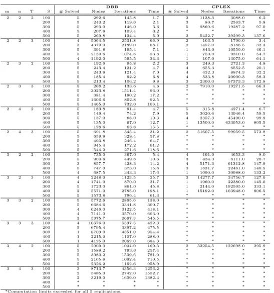
The results of the experiments appear in full in Table 1. Statistics on the num-ber of instances solved and premature terminating conditions can be found in Table 2. As evident from the tables, the numerical results for the DBB Al-gorithm are quite positive. The alAl-gorithm performed significantly better than CPLEX in its efforts to solve the deterministic equivalent in all three of the per-formance measures. Nearly 85% of the instances were solved within the desired tolerance by the algorithm within the time, iteration and node constraints that were set a priori. Of those that did not fully solve, only 38% were terminated prematurely due to time. The average gap between the bounds after stopping due to the time constraint was a reasonable 2.05%. When the termination was due to a memory problem or node limitation the average stopping time was 882.3 seconds and the average gap was 1.10%.
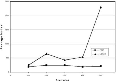
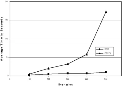
CPLEX MIP statistics are extremely unfavorable. The problem becomes unsolvable for CPLEX rather quickly, evident by the lack of numbers in Table DBB. Its success rate was a mere 27%, and over 90% of its premature termi-nations were due to time with an average stopping gap of 0.848%. As one can see from Table 1, the number of scenarios in general has a much greater impact on the CPLEX MIP, where the effect on the DBB Algorithm is not as drastic. In order to illustrate the differences in the two, the set of instances in which CPLEX could be most closely compared to the algorithm were examined. The case of 2 resources, 3 tasks, and 2 time periods is the one in which CPLEX solved the most instances of any set of problem parameters. Figures 1 through 3 compare the performance of both algorithms in terms of three performance measures. The rapid growth of nodes, iterations and solution time evident in the CPLEX runs is more severe than the that of the DBB algorithm values. In total, of the 253 instances solved by the DBB Algorithm, the solution time surpassed the CPLEX MIP time on only 4 occasions, and was beaten 9 times in all 300 runs. The average time savings in those 9 instances for CPLEX was 191.2 seconds.
DBB CPLEX
m n T S # Solved Nodes Iterations Time # Solved Nodes Iterations Time 2 2 2 100 5 292.6 145.8 1.7 3 1138.3 3088.0 6.2 200 5 240.2 119.6 2.1 3 80.7 2563.7 5.8 300 5 293.0 146.0 3.6 5 9860.6 19287.2 97.0 400 5 207.8 103.4 3.2 * * * * 500 5 269.8 134.4 5.0 3 5422.7 39299.3 137.6 2 2 3 100 4 5064.5 2531.8 66.9 2 103.5 1790.0 3.4 200 3 4379.0 2189.0 68.1 2 1457.0 8186.5 32.3 300 5 391.8 195.4 7.1 1 843.0 10550.0 46.1 400 5 2150.6 1074.8 53.8 1 750.0 9310.0 54.7 500 4 1192.0 595.5 33.3 1 107.0 13075.0 64.1 2 3 2 100 5 192.6 95.8 2.2 3 249.3 2721.3 4.8 200 5 243.4 121.2 4.7 4 655.3 6552.5 20.1 300 5 243.8 121.4 7.0 4 432.3 8874.3 32.2 400 5 185.4 92.2 6.8 4 533.8 20990.3 58.3 500 5 213.4 106.2 9.8 3 2300.0 57373.3 172.8 2 3 3 100 5 268.2 133.6 4.6 2 7910.0 19271.5 66.3 200 5 3023.8 1511.4 96.0 * * * * 300 5 381.4 190.2 17.2 * * * * 400 5 1606.6 802.8 92.5 * * * * 500 5 1465.0 732.0 103.1 * * * * 2 4 2 100 5 183.8 91.4 4.7 5 315.8 4271.4 6.7 200 5 149.4 74.2 7.9 5 3020.6 13946.4 59.5 300 5 137.0 68.0 10.3 4 2357.3 45490.0 99.9 400 5 135.0 67.0 12.7 1 13500.0 633953.0 805.5 500 5 128.6 63.8 15.5 * * * * 2 4 3 100 5 691.8 345.4 31.2 2 51607.5 99959.5 573.8 200 5 659.8 329.4 57.8 * * * * 300 5 493.8 246.4 64.7 * * * * 400 5 345.4 172.2 61.2 * * * * 500 5 544.2 271.6 118.6 * * * * 3 2 2 100 5 735.0 367.0 5.4 4 191.0 4653.3 8.0 200 5 900.6 449.8 10.6 3 434.3 8111.0 28.7 300 3 857.7 428.3 14.2 4 5171.3 61312.8 147.9 400 5 747.0 373.0 15.8 3 1831.7 22461.0 140.5 500 4 687.5 343.3 17.6 1 1090.0 30988.0 133.2 3 2 3 100 4 2248.0 1123.5 25.7 3 14277.7 34756.7 127.0 200 4 1741.0 870.0 31.7 1 1960.0 22380.0 145.0 300 5 1723.0 861.0 45.8 1 2144.0 192505.0 333.1 400 2 5571.0 2785.0 198.1 1 15192.0 103948.0 806.5 500 5 1573.8 786.4 61.3 * * * * 3 3 2 100 5 5772.6 2885.6 138.0 * * * * 200 5 6684.6 3341.8 300.7 * * * * 300 4 6246.0 3122.5 418.1 * * * * 400 4 7141.0 3570.0 603.0 * * * * 500 3 5375.7 2687.3 545.5 * * * * 3 3 3 100 4 10676.0 5337.5 422.3 * * * * 200 5 6795.4 3397.2 475.5 * * * * 300 1 8703.0 4351.0 954.4 * * * * 400 1 2215.0 1107.0 288.0 * * * * 500 1 4125.0 2062.0 684.3 * * * * 3 4 2 100 5 2009.0 1004.0 169.3 2 33254.5 122698.0 295.9 200 5 1588.2 793.6 257.4 * * * * 300 5 3080.2 1539.6 781.0 * * * * 400 5 2165.8 1082.4 710.5 * * * * 500 5 2326.2 1162.6 958.0 * * * * 3 4 3 100 3 8713.7 4356.3 1256.2 * * * * 200 2 5485.0 2742.0 1552.7 * * * * 300 2 3219.0 1609.0 1382.4 * * * * 400 * * * * * * * * 500 * * * * * * * *
*Computation limits exceeded for all 5 replications.
Table 1: Numerical results
DBB CPLEX
Reason for Termination Instances % Avg Gap Avg Time Instances % Avg Gap Avg Time Solved 253 84.3 0.005 173.9 81 27.0 0.008 105.3 Time 18 6.0 2.046 1800.0 198 66.0 0.848 1800.0 Nodes or Iterations 8 2.7 0.662 452.5 21 7.0 0.065 1256.0 Memory 21 7.0 1.264 1046.0 0 0.0 * * *Not Applicable.
Figure 1: Number of Nodes.
Figure 3: CPU time.
5.4
Interpretation
In problems of this size and parameter range, it is favorable to use the DBB Algorithm rather than conventional MIP solution strategies. The DBB algo-rithm’s performance was superior in virtually every problem instance without the assistance of any preprocessing or advanced memory management. The number of scenarios seems to be the greatest stumbling block for CPLEX. This is the parameter that grows most rapidly in common applications of this type, hence, it is crucial to establish an algorithm that is less sensitive to scenario growth. The DBB Algorithm’s major factor is actually the interaction between a combination of 2 problem parameters. The number of variables to be branched upon in the first stage MIP is determined by the number of resources and the number of time periods.
The other significant parameter combination is that of resources and tasks, which drastically changes the size of the solution search space in the enumeration scheme used to solve the general assignment subproblems in the second stage. One immediate improvement to the algorithm is to generate a more efficient solution strategy to these subproblems; if the time needed to solve them is improved, a considerable reduction in overall solution time might be achieved. Growth in the algorithms branch-and-bound iterations was not that significant when compared to the solution time as problem sizes increased. This is due in large part to the solution time required of the subproblems, which must be solved for each scenario at every iteration. Some alternate approaches might be
to use dynamic programming methods, or solve these problems using a heuristic and possibly obtain an approximate solution to the entire problem.
CPLEX MIP, while only solving 27% of the problems, seemed to tighten the bounds rather quickly even when the problems were not solved within the allot-ted time. The natural tendency was to make great improvements rather quickly and then slowing to almost a halt, with the gap remaining almost constant. The DBB Algorithm, on the other hand, seemed to keep a steady pace while converg-ing. A possibility for improvement may be to use a generic branch-and-bound approach such as CPLEX MIP in conjunction with the DBB algorithm. The generic approach could be used to find an initial feasible solution for the DBB algorithm with tight bounds, and then a hot start would place the algorithm in a much more advantageous position.
The number of scenarios becomes the crucial parameter in deciding which modeling approach and solution strategy to pursue. Several trial runs were con-ducted on smaller instances where this parameter was in the ranges of 20 to 50 scenarios. Although, the DBB Algorithm also solved these problems rather quickly, CPLEX seemed to outperform the algorithm on average. As this param-eter increases, the problem becomes unsolvable for a general branch-and-bound approach and use of the algorithm becomes the appropriate scheme.
6
Concluding Remarks
In this paper we have developed a model for dynamic capacity acquisition and allocation under uncertainty. The resulting problem is a two-stage stochastic integer program, which is extremely difficult to solve. We used a recently de-veloped decomposition based branch and bound algorithm to solve this class of problems to global optimality. Our preliminary numerical experiments suggest significant saving in computational effort when using the proposed decomposi-tion strategy over straight-forward use of commercial solvers.
References
[1] S. Ahmed, M. Tawarmalani, and N.V. Sahindis. A finite branch and bound algorithm for two-stage stochastic integer programs. Stochastic Program-ming E-Print Serieshttp://dochost.rz.hu-berlin.de/speps/, 2000. [2] O. Berman, Z. Ganz, and J. M. Wagner. A stochastic optimization model
for planning capacity expansion in a service industry under uncertian de-mand. Naval Research Logistics, 41:545–564, 1994.
[3] J. R. Birge and F. Louveaux. Introduction to Stochastic Programming. Springer, New York, NY, 1997.
[4] J. R. Birge and F. V. Louveaux. A multicut algorithm for two-stage stochas-tic linear programs. European Journal of Operational Research, 34(3):384– 392, 1988.
[5] C. E. Blair and R. G. Jeroslow. On the value function of an integer program.
Mathematical Programming, 23, 1979.
[6] C. C. Caroe.Decomposition in stochastic integer programming. PhD thesis, University of Copenhagen, 1998.
[7] C. C. Caroe and J. Tind. L-shaped decomposition of two-stage stochastic programs with integer recourse. Mathematical Programming, 83:451–464, 1998.
[8] Y. Ermoliev. Stochastic quasigradient methods and their application to systems optimization. Stochastics, 9:1–36, 1983.
[9] C. O. Fong and V. Srinavasan. The multiregion dynamic capacity expansion problem: Part I. Operations Research, 29:787–799, 1981.
[10] C. O. Fong and V. Srinavasan. The multiregion dynamic capacity expansion problem: Part II. Operations Research, 29:800–816, 1981.
[11] J. L. Higle and S. Sen. Stochastic decomposition: An algorithm for two stage stochastic linear programs with recourse. Mathematics of Operations Research, 16:650–669, 1991.
[12] R. Horst and H. Tuy. Global Optimization: Deterministic Approaches. Springer-Verlag, Berlin, 3rd edition, 1996.
[13] Gerd Infanger. Monte Carlo (importance) sampling within a Benders de-composition algorithm for stochastic linear programs.Annals of Operations Research, 39(1-4):69–95, 1993.
[14] J. G. Klincewicz, H. Luss, and C.-S. Yu. A large-scale multilocation capac-ity planning model.European Journal of Operational Research, 34:178–190, 1988.
[15] G. Laporte and F. V. Louveaux. The integer L-shaped method for stochas-tic integer programs with complete recourse. Operations Research Letters, 13:133–142, 1993.
[16] S.-K. Lim and Y.-D. Kim. An integrated approach to dynamic plant lo-cation and capacity planning. Journal of Operational Research Society, 50:1205–1216, 1999.
[17] M. L. Liu and N. V. Sahinidis. Optimization in process planning under uncertainty. Industrial & Engineering ChemistryResearch, 35:4154–4165, 1996.
[18] V. I. Norkin, G. C. Pflug, and A. Ruszczynski. A branch and bound method for stochastic global optimization.Mathematical Programming, 83:425–450, 1998.
[19] A. Ruszczynski. A regularized decomposition method for minimizing a sum of polyhedral functions. Mathematical Programming, 35:309–333, 1986. [20] R. Schultz. Continuity properties of expectation functions in stochastic
integer programming.Mathematics of Operations Research, 18(3):578–589, 1993.
[21] R. Schultz. On structure and stability in stochastic programs with random technology matrix and complete integer recourse. Mathematical Program-ming, 70(1):73–89, 1995.
[22] R. Schultz, L. Stougie, and M. H. van der Vlerk. Solving stochastic pro-grams with integer recourse by enumeration: A framework using Gr¨obner basis reductions. Mathematical Programming, 83:229–252, 1998.
[23] A. Shapiro and Y. Wardi. Convergence analysis of gradient descent stochas-tic algorithms. Journal of Optimization Theoryand Applications, 91:439– 454, 1996.
[24] J. M. Swaminathan. Tool capacity planning for semiconductor fabrica-tion facilities under demand uncertainty. European Journal of Operational Research, 120:545–558, 2000.
[25] R. Van Slyke and R. J.-B. Wets. L-Shaped linear programs with applica-tions to optimal control and stochastic programming. SIAM Journal on Applied Mathematics, 17:638–663, 1969.