An evaluation of using
GPM satellite products to
forecast flash floods in
mountainous catchments
________________________________________________
Yihan Chen
Master Thesis
TVVR 17/5020
An evaluation of using
GPM satellite products to
forecast flash floods in
mountainous catchments
By:
Yihan Chen
Master Thesis
Division of Water Resources Engineering
Department of Building & Environmental Technology
Lund University
Box 118
Water Resources Engineering
TVVR 17/5020
ISSN 1101-9824
Lund 2017
www.tvrl.lth.se
Master Thesis
Division of Water Resources Engineering
Department of Building & Environmental Technology
Lund University
English title:
An evaluation of using GPM satellite products to
forecast flash floods in mountainous catchments
Author(s):
Yihan Chen
Supervisor:
Dr. Rolf Larsson
Assoc. Prof. Fuqiang Tian
Examiner:
Linus Zhang
Language:
English
Year:
2017
Acknowledgements
I would like to thank Associate Prof. Fuqiang Tian (Tsinghua University,
Department of Hydraulics) and Associate prof. Rolf Larsson (Lund university,
Water resource engineering) for supervising me on this thesis. I would also
like to thank the examiner of this thesis, Associate Prof. Linus Zhang.
Furthermore I would like to express my gratitude to Yilu Li, Shiyou Hou and
Sihan Zhao for helping me with input data and the hydrological model.
Abstract
NASA's GPM satellite rainfall products IMERG early run and IMERG late run
were evaluated for their applicability in flash flood forecasting. The selected
catchment was the upper Han River basin, a mountainous catchment with low
precipitation in winter and heavy precipitation during summers located in
central China. The evaluated period spanned from 2015-03 to 2016-03 and is
limited by the IMERG data history. The hydrological model that was used to
simulate river floods was the THREW model. The IMERG data was first
compared to data from rain gauges at an hourly 0.1x0.1 degree grid scale. The
comparison criteria were correlation (r
2), relative root mean squared error
(RMSE) and mean bias (BIAS). The errors between IMERG and rain gauges
were also compared against elevation. The results showed that the correlation
varied from 0.3 to -15 (late run) and 0.33 to -21 (early run), relative RMSE
varied from 730 % to 4100 % (early run), bias varied from -25 % to 370 %
(early run) and -19 % to 410 % (late run),
Then, using the bias factor correction method, the two IMERG data sets were
corrected against the rain gauge data set.
Simulations of river flows during 2015-03 to 2016-03 with the prepared
precipitation data sets showed that the uncalibrated IMERG data performed
with a Nash-Sutcliffe Model efficiency of -8 and -10 (early and late) while rain
gauges performed 0.19. The calibrated IMERG performed -0.14 and -0.21
(early and late) which was a considerably improvement from the uncalibrated
IMERG. Simulation results showed that while the near-real time products
IMERG early and IMERG late have potential to estimate rain events that
generate floods, calibration of the IMERG products are necessary in order to
set reasonable results.
Contents
Acknowledgements i Abstract ii List of Figures v List of Tables vi Abbreviations vii 1 Introduction 1 1.1 Background . . . 1 1.2 Aim . . . 2 1.3 Procedure . . . 2 1.4 Limitations . . . 3 2 Study area 4 2.1 The upper Han river . . . 43 Global Precipitation Measurement mission (GPM) 6 3.1 History . . . 6
3.2 Technical specifications . . . 6
3.3 Current research in IMERG . . . 8
3.4 Hydrological application of IMERG . . . 8
3.5 Early/late runs vs. final run . . . 8
4 TsingHua Representative Elementary Watershed model (THREW) 9 4.1 General model structure . . . 9
4.2 Vegetated zone and bare soil zone (v-zone, b-zone) . . . 11
4.3 Unsaturated and saturated zone (u-zone, s-zone) . . . 13
4.4 Sub-stream and main channel zone (t-zone, r-zone) . . . 15
4.5 The upper Han river model specifics . . . 18
5 Data and methods 20 5.1 IMERG . . . 20
5.2 Rain gauges . . . 21
Contents iv
5.4 Reference evapotranspiration . . . 24
5.5 Discharge data . . . 26
5.6 Quantifying performance of the hydrological model . . . 26
6 IMERG analysis and correction 28 6.1 Error analysis . . . 28
6.2 Error correction . . . 34
7 Results and Discussion 35 7.1 Upper Han river model results using rain gauge precipitation data as forcing 35 7.2 Performance of the hydrological model with IMERG precipitation data . . 36
7.3 Sources of errors . . . 41
7.3.1 Discharge data . . . 41
7.3.2 Rain gauge data . . . 41
7.3.3 Reference evapotranspiration . . . 42
7.4 IMERG correction method . . . 42
7.5 Interpolation methods . . . 43
8 Conclusion 44 8.1 Using IMERG for flood prediction . . . 44
8.2 Further research . . . 44
A FAO 56 Penman-Montieth calculation process 46
List of Figures
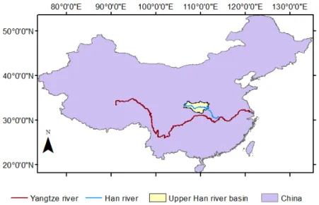
2.1 Yangtze river and the Han river with the upper Han river basin . . . 4
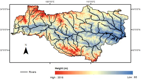
2.2 The upper Han river basin and its elevation . . . 5
3.1 The GPM satellite constellation . . . 7
4.1 A basin split in REW units . . . 9
4.2 Regions in the REW unit . . . 10
4.3 Simplified surface geometry of a REW . . . 11
4.4 Overview of REW and zone interactions . . . 11
4.5 The upper Han river basin divided into 89 REWs . . . 19
5.1 GPM grid over the upper Han river basin . . . 20
5.2 Usable gauges in the upper Han river . . . 22
5.3 Area of influence using Thiessen polygon . . . 23
5.4 MODIS 15 reference system . . . 23
5.5 a) Example of a 4-day composite of leaf area index in the upper Han river basin b)Resulting REW averaged LAI of a) . . . 24
5.6 Meteorological stations in the upper Han river region . . . 25
5.7 Hydrological stations on the upper Han river basin . . . 26
6.1 The spatial variation of total precipitation volume for the period March 2015 to February 2016 for a) gauges b) IMERG early(6h) c) IMERG late(18h) . . . 30
6.2 Analysis of IMERG errors and its’ attributes, a-b) Relative errors of IMERG early and late plotted against elevation c-d) IMERG precipta-tion data plotted against rain gauge precipitaprecipta-tion data e-f) accumulated difference between IMERG and intersecting rain gauge . . . 31
6.3 Statistical indicators for IMERG early run and late run interpolated to a continuous field over the upper Han river basin . . . 33
7.1 Simulated discharge with rain gauges compared to observed discharge in the upper Han river basin (hourly time steps) . . . 35
7.2 Simulated discharge of uncalibrated IMERG early(6h) run and late (18h) run compared to observed discharge . . . 37
7.3 Simulated discharge of uncalibrated IMERG early(6h) run and late (18h) run compared to rain gauge-simulated discharge . . . 38
7.4 Simulated discharge with calibrated IMERG precipitation data compared to observed discharge . . . 39 7.5 Simulated discharge with calibrated IMERG precipitation data compared
List of Tables
3.1 Different versions of IMERG and their attributes . . . 7
4.1 Zones with their corresponding location and abbreviation . . . 10
5.1 GPM grid limit . . . 20
5.2 CMA weather station data declaration . . . 25
6.1 Detection accuracy of IMERG early and late to rain gauges, i.e. detection matrix . . . 30
6.2 Statistical indicators between rain gauges and IMERG . . . 32
7.1 Statistical indicators of the performance of rain-gauge driven hydrological model in comparison to observed discharge data . . . 36
7.2 Statistical indicators of the performance of IMERG driven hydrological model in comparison to observed discharge data . . . 38
7.3 Statistical indicators on the comparison of simulated discharge driven by calibrated IMERG data with observed discharge and with rain gauge-driven discharge simulation respectively . . . 40
Abbreviations
GPM GlobalPrecipitation Measurement mission
IMERG IntegratedMulti-satellitE Retrieval for GPM
LAI Leaf Area Index
REW Representative Elementary Watershed
IDW Inverse Distance Weighting
NSC Nash-Sutcliffe model efficiencyCoefficient
RMSE RootMeanSquaredError
CC Correlation Coefficient
Chapter 1
Introduction
1.1
Background
Extreme weather events in China cause deaths and property damage almost yearly. The most common type of natural disaster due to these events in China is flooding. In 1931 it is estimated that somewhere between 900 000 to 4 million people died during the world’s deadliest flooding which took place in China [Britannica, 2016]. Just this year (2016), over a hundred have died and billions(U.S. dollar) of properties were damaged due to flooding [Aon-Benfield, 2016].
The most dangerous type of flooding is flash floods. Flash floods are characterized by fast arising destructive currents that pose a major risk to both property and human lives. Flash floods are usually caused by heavy rainfall over a short period but can also be caused by an accidental release of water from storage, i.e. dam breakage [NSSL, 2016].
To prevent the loss of human life and mitigate damage to property, prediction of flash floods are important. Forecasting a flash flood will increase the ability to evacuate people early from the affected area. A common practice to forecast flash floods is to establish a hydrological model that relies on rainfall forcing in order to predict flooding events. Often rainfall data is obtained through in-situ measurements. These are usually from rain gauges which report the rainfall amount with a certain time interval. The density of rainfall gauges is crucial to the outcome of the model. The higher density of rainfall gauges in a basin the more likely the model is to achieve accurate results. The amount of rainfall gauges can, however, be limited by accessibility and resources. This leads to basin areas where the gauge density is low and thus the network of gauges will be
Introduction
One other important aspect is the lead time of the data. It is crucial, when predicting flash floods, to get rainfall data as early as possible due to the short time of its arising (as opposed to regular floods that can be predicted days ahead). Rain gauges that are not measuring real time can have a hard time in fulfilling this requirement.
To achieve good model results and lead time for areas that lack rain gauges other means of measurement methods such as radar and satellite products may be used.
One of such satellite products, which is fairly new (launched 2014) is the Global Pre-cipitation Measurement mission. The product is provided for free by U.S. NASA and is the satellite product to be evaluated in this thesis. [NASA, 2011a]
1.2
Aim
The main goal of this thesis is to evaluate the applicability of GPM satellite rainfall products to forecast flash floods in mountainous catchments, in comparison to using gauged precipitation data. A method for improving the GPM product using gauges as reference is also to be evaluated. Questions to be investigated:
• How does the GPM product perform (for flood prediction) in comparison to rain gauges in high density gauge network?
• How well does rainfall estimates from the GPM product correlate with rain gauge data?
• Can the flood prediction be improved when combining the GPM product with rain gauge data?
• What is the viability of the GPM product for predicting flash floods?
1.3
Procedure
Firstly, A hydrological model will be established for a well gauged mountainous catch-ment using data from rain gauges. This hydrological model will be used for evaluating the performance of GPM products. Secondly, the same hydrological model will be driven by GPM rainfall products. A satellite-rain gauge correction method will be applied to the input data at this step in order to increase model performance. The performance of this satellite-rain gauge forced hydrological model will then be compared to the same hydrological model driven solely by gauged precipitation data. The main indicator of performance will be the Nash-Sutcliffe model efficiency coefficient. Lastly, an evaluation of the applicability of using GPM rainfall products for flash flood forecasting will be
Introduction
1.4
Limitations
Due to the limitations of a master thesis, a basin which already has an established and good performing model will be used. Using an already established model will save time as opposed to building one from scratch which requires a lot resources. By same limitation, the GPM-gauge correction method used in this thesis has to be fairly simple.
Chapter 2
Study area
2.1
The upper Han river
For evaluating the GPM products in mountainous catchments an appropriate basin has to be chosen. There are a lot of mountainous catchments in China but the upper Han river basin is deemed as the best for this thesis. The reason for choosing upper Han river basin is that it is extensively researched. The extensive research done on this area can aid in the evaluation of results produced by this thesis project. The density of the gauge network in this catchment is high and there are six hydrological stations in this basin that measure the river flow. There is also already a model established for this basin by the Hydrology group at the Department of Hydraulic Engineering at Tsinghua University, which reduces the amount of preparation needed in order to carry out the evaluations.
Study area
The upper Han river basin is the most upstream part of the Han river. The Han river is located in central china and is a major tributary of the Yangtze river (see fig. 2.1). It originates in Qin mountains of Shaanxi province and stretches 1500 km to the Yangtze river at the city of Wuhan in Hubei province.
Figure 2.2: The upper Han river basin and its elevation
From its start to outlet the upper Han river drops from 2000 m.a.s.l. to 150 m.a.s.l. The outlet of the upper Han river basin is located at the Danjiangkou reservoir. The basin has an area of 95 200 km2 with the main river running 900 km from west to east. The climate in the upper Han river basin is sub-tropical with heavy rainfall in summer and dry periods in winter. In this basin there are many reservoirs that regulate the flow in the main river with Danjiangkou being the biggest.
The upper Han river is prone to flooding due to its mountainous landscape and heavy summer rainfall, which further argues for this basin as an ideal study area.
Chapter 3
Global Precipitation
Measurement mission (GPM)
3.1
History
In 1997 U.S. NASA and Japanese JAXA launched together satellites in what would be the Tropical Rainfall Measurement mission (TRMM). The mission was to achieve a better understanding how water moves around at a global scale using remote sensing. The TRMM was estimating rainfall in earth’s tropical zones until 2014 when it was replaced by the Global Precipitation Measurement mission. The Global Precipitation Measurement mission uses a constellation of satellites from different providers and a main calibrating satellite in order to produce near real time precipitation estimates. The estimation is done by measurements from two instruments, the GPM Microwave Imager from the main satellite and the Dual-Frequency Precipitation Radar on the remaining satellites. These measurements are run through a series of algorithms in order to arrive at the final precipitation estimation. [NASA, 2011a]
3.2
Technical specifications
GPM products are provided in different levels and versions. Levels 1 to 3 represent the different processing stages of satellite data in which the third level is the precipitation product.[NASA, 2011b]
Level 1 which is the lowest level, contains only raw GPM microwave imagery data. At level 2 the raw data has been translated into parameters concerning rainfall. There are different versions at this level which reflect each of the sensors and frequency bands and the combinations of those.
Global Precipitation Measurement mission (GPM)
Figure 3.1: The GPM satellite constellation [NASA, 2017]
At level 3 all estimates are merged and interpolated to create precipitation estimations. At this level the versions differ by which sensors are merged. The most accurate pre-cipitation product at level 3 is the Day-1 IMERG prepre-cipitation set. This data set is an interpolation and merging of all sensors. The data set comes at 0.1 [degrees] spa-tial resolution and different temporal resolutions at 30 min, 3 hours, daily, 7-day and monthly. The IMERG product is provided in near real time and post real time. The fastest data product at this level is called IMERG early run and has a six hour time lag (long term goal of 4 hours according to NASA) between recorded event and publication. The second fastest is the IMERG late run with 18 hours delay (long term goal of 12 hours). The third and slowest IMERG product is the final run which has a delay of 4 months. IMERG early and late run are considered to be near-real time while IMERG final run is a post-real time product. [Huffman et al., 2015]
Table 3.1: Different versions of IMERG and their attributes
Run Delay Spatial resolution Temporal resolutions Accuracy Early 6 hours 0.1x0.1 [degrees] 30 min, 3 hours, 1 day,
3 days, 7 days Worst Late 18 hours 0.1x0.1 [degrees] 30 min, 3 hours, 1 day,
3 days, 7 days Medium Final 4 months 0.1x0.1 [degrees] 30 min, 1 day, monthly Best
Global Precipitation Measurement mission (GPM)
3.3
Current research in IMERG
Since IMERG is fairly new, research on the hydrological forecasting performance of IMERG early run and late run are limited. However, there are plenty of research (such as [Guoqiang et al., 2016] [Rios Gaona et al., 2016] [Chen and Li, 2016]) that evaluates the IMERG final run in comparison to gauges and the common conclusion is that the IMERG final run looks promising for use in analyzing floods/draughts. However same studies mention that IMERG is far from perfect and should be improved further for more accurate predictions. Guoqiang et al. [2016] also show that the errors in IMERG final run is related to precipitation, climate, intensity, elevation, temporal scale and randomness.
In China, Guoqiang et al. [2016] show that IMERG final run performance is influenced by climate and temporal scale. IMERG final run at an hourly scale performs poorly in comparison to the daily scale. Guoqiang et al. [2016] divided China into six regions for which each region were tested for correlation and errors. There was no region that specifically contained the upper Han river basin. There are however two regions close to the upper Han river basin. These two regions performed relatively well (in comparison to other regions) at a daily scale. They also performed better at an hourly scale in comparison to the rest.
3.4
Hydrological application of IMERG
For hydrological application, Lia et al. [2017] used IMERG final run to predict stream flows in the Ganjiang. Ganjiang is also a tributary of Yangtze river but is located on the south side. The IMERG final run performed worse than gauges and gauge-calibrated radar but was still applicable for stream flow prediction. Even though IMERG final run is subject to errors, it still has potential for hydrological applications Lia et al. [2017].
3.5
Early/late runs vs. final run
The studies that have been presented in this section all make use of the final run of IMERG. As mentioned in section (3.2), the final run is the most accurate IMERG version. For the early run and late run the errors should be bigger. The difference in errors between early/late and final is due to the calibration of data with rain gauges, which is not done for the early/late runs. Thus the early/late runs are expected to have larger errors than the final run [Huffman et al., 2015].
Chapter 4
TsingHua Representative
Elementary Watershed model
(THREW)
4.1
General model structure
THREW, an acronym for Tsing Hua Representative Elementary Watershed, is a phys-ically semi-distributed hydrological model developed at the Department of Hydraulic Engineering at Tsinghua University. It is an extension of the original Representative Elementary Watershed (REW) by Paolo Reggiani. [Tian et al., 2008]
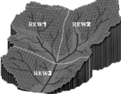
Figure 4.1: A basin split in REW units
THREW adheres to the principle of a continuous open system thermodynamic model. Mass, momentum and heat are preserved throughout the system. The model uses dis-crete elements, henceforth referred to as REWs, to model runoff in river basins (Figure 4.1). Each REW is considered to be a sub basin of the larger basin model and thus has
TsingHua Representative Elementary Watershed model (THREW)
Figure 4.2: Regions in the REW unit
Each REW is in turn divided into eight zones (fig. 4.2), that are necessary for describing the hydrological processes. These zones can be categorized into two layers, the surface layer and the subsurface layer.
The surface layer consists of the following six zones, snow zone, glacial zone, vegetated zone, bare soil zone, sub-stream zone and main channel zone. The subsurface layer consists of two zones saturated zone and unsaturated zone.
Table 4.1: Zones with their corresponding location and abbreviation
Layer Zone Abbreviation
surface snow n glacial g vegetated v bare soil b sub-stream t main channel r sub-surface unsaturated u saturated s
The surface geometry of each sub-basin is simplified into an open triangular channel (fig. 4.3). This simplified surface geometry model has a reference system defined in figure. Determining bank angles (γr,γt) can be done through slope analysis with a digital elevation model.
Hydrological processes for each zone are described by physically based equations for mass, momentum and heat balance. The exchange between each zones are schematically described in figure 4.4
TsingHua Representative Elementary Watershed model (THREW)
Figure 4.3: Simplified surface geometry of a REW
Figure 4.4: Overview of REW and zone interactions
This system of equations are simplified through empirical relationships and assumptions. The resulting system is an ordinary differential equation system. In each section of this chapter, the general balance equation with their empirical relationships are presented for each zone. Since the Han river-model does not account for snow and glacial zones these processes and heat balance will not be described in this thesis.
4.2
Vegetated zone and bare soil zone (v-zone, b-zone)
The vegetated and bare soil zone are volumes in the surface layer that are responsible for hydrological processes such as evaporation, transpiration, depression and interception. The area of vegetated zone is dynamic and varies by season and year. In the vegetated zone the outgoing fluxes are due to transpiration and evaporation. Water is extracted from the unsaturated zone by vegetation and is transpired into the air. Water can alsoTsingHua Representative Elementary Watershed model (THREW)
in processes between b-zone and v-zone they can be defined with a combined equation where j denotes the sum of v-zone and b-zone.
d dt(y
jωj) =ejP +eju+ejt+ej
lg (4.1)
yj : soil depth of j-zone [length]
ωj : area ratio of j-zone
ejp : precipitation falling on j-zone
eju : mass exchange between u-zone and j-zone
ejt : Hortonian runoff to the j-zone
ejlg : evaporation/transpiration from j-zone
Evaporation and transpiration (ejlg) is limited by either the reference evapotranspiration or by the exfiltration capacity of the soil in the u-zone.
evlg=min (1−M)Ep+M(ETv) ·ωj, fe·ωj (4.2)
Where M is the fraction of vegetation,ETv is the reference evapotranspiration,feis the
exfiltration capacity of the unsaturated zone. Governing equation for the exfiltration capacity can be found in section (4.3) equation (4.8).
Interception is subtracted from the precipitation falling on the v-zone and can be defined as:
V =Sm(1−e−p/Sm) +ω·ETp (4.3)
p: precipitation
Sm : interception coefficient ETp : potential evapotranspiration
Sm=α·LAI (4.4)
α: coefficient for leaf area index
Where the LAI is the leaf area index that is input into the model and p is the rainfall. The bare soil zone is the zone that is only defined by the absence of the other six zones in the surface layer. This means that the bare soil zone is the area left in the surface layer which cannot be categorized in any of the other zones. This zone has storage and
TsingHua Representative Elementary Watershed model (THREW)
mass exchange in the form of depression and evaporation/infiltration only. Thus for the bare soil zone the fraction of vegetation is 0. No interception happens in this zone. The depression storage in the b-zone is empirically set to around 1-2 mm for impermeable surfaces and 2-15 mm to permeable surfaces. When the depression storage is exceeded, the water will directly go to the sub-stream zone see section (4.4)
4.3
Unsaturated and saturated zone (u-zone, s-zone)
The unsaturated and saturated zones are responsible for hydrological processes in the ground. Zones are separated by the ground water table which fluctuates over the year. The saturated zone is limited by the bedrock at the bottom which is assumed to be flat in the THREW model. In the saturated zone, vertical momentum is neglected while in the unsaturated zone horizontal momentum is neglected. Rainfall that reaches the unsaturated zone infiltrates to the saturated zone and adds to the height of water table. From the saturated zone mass exchange occurs with neighbouring REW’s saturated zone and the main channel zones.
The general equation for mass balance can be defined for u-zone as:
d dt(
usuyuωu) =eus+eub+euv (4.5)
u : volume of soil moisture in u-zone
su : soil moisture in u-zone [volume]
yu : soil depth of u-zone [length]
ωu : area ratio of u-zone
eus : mass exchange between s-zone and u-zone
eub: mass exchange between b-zone and u-zone
euv: mass exchange between v-zone and u-zone
Mass exchange between the u-zone and surface layers (euv,eub) are governed by
infiltra-tion and exfiltrainfiltra-tion. The infiltrainfiltra-tion in the unsaturated zone is defined as:
fi=Ku s 1 +αIF L|ψ|(1−s u)u suyu (4.6)
TsingHua Representative Elementary Watershed model (THREW)
Ks
u : hydraulic conductivity in the unsaturated zone
αIF L: infiltration coefficient
ψ: averaged water potential in u-zone
However the actual infiltration is limited by the water supply. There can never be more infiltration than what is provided through rain, storage depletion and irrigation. The actual infiltration is thus:
Fj =minRωj, fiωj
(4.7) Where R is the water supply in the form of either rain, depression storage or irrigation. If R exceeds the infiltration capacity, the water will go directly to depression storage. Exfiltration is due to vegetation extracting water from the u-zone:
fe=α
Kus
(1−su)yu ·
(su)2+du|ψb|
µ (4.8)
ψb : entry suction value for air
µ: soil pore distribution index
d: diffusion index
Where the relationship between the soil pore distribution index and the diffusion index:
d= 2 + 1/µ (4.9)
The unsaturated and saturated zone exchanges water through recharge and capillary rising (eus):
eus =αωvz (4.10)
α : coefficient for recharge/capillary rising
: volume of soil moisture in u-zone
vz : velocity of water flow in u-zone
The velocity of the water flow in the u-zone is solved through momentum balance and can be defined as:
vz =K u su 0.5 +ψ u yu (4.11)
TsingHua Representative Elementary Watershed model (THREW)
The mass balance equation for the s-zone can be defined as:
d dt(
sysωu) =esu+est+esr (4.12)
u : volume of soil moisture in s-zone
ys : soil depth of s-zone [length]
ωs: area ratio of s-zone
esu : same aseus see equation (4.10)
est : water flow from the s-zone to the t-zone (Dunnian runoff)
esr : mass exchange between r-zone and s-zone
The water can seep from the s-zone onto the surface and create or add to sub-streams (est). This happens where the height of the water table is higher both the surface and the r-zone. This process is also known as Dunnian runoff and is specially important in mountainous areas. est =αstKss ys Z βst (4.13)
αst: coefficient for seepage
βst : empirical coefficient
Kss: average saturated hydraulic conductivity for s-zone
Z : total soil depth
For water flow from the saturated zone to the main channel (i.e. esr) the defining equation is the same as equation (4.13) but with different empirical coefficients (α and
β).
4.4
Sub-stream and main channel zone (t-zone, r-zone)
The main channel is connected throughout the network of REWs. It is subsequently the river for which the flow is modeled. The main channel exchanges mass with the saturated zone and main channels from neighbouring REWs. The sub-stream zone represents small streams and lakes/reservoirs that are located within the REW. The sub-streamsTsingHua Representative Elementary Watershed model (THREW)
The governing equation for mass balance for the t-zone:
d dt(y
tωt) =ept+etb+etv+ets+etr+et
lg (4.14)
yt: average water depth of t-zone [length]
ωt: area ratio of t-zone
ept: precipitation falling on t-zone
etb: Hortonian runoff from b-zone to t-zone
etv: Hortonian runoff from v-zone to t-zone
ets: Dunnian runoff from s-zone to t-zone, see equation (4.13)
etr : Diversion from t-zone to r-zone
etlg: evaporation from t-zone
When the rainfall intensity exceeds the infiltration capacity and depression storage of the soil, the water runs directly to the t-zone. This process is called Hortonian runoff (etb,etv) and happens only from the b-zone and v-zone in the surface layer. The evaporation from the t-zone (etlg) is identical to the evaporation process from the b-zone (section 4.2) The area ratio of the t-zone (ωt) is defined by the relationship of geometric and volu-metric properties of the sub-surface layer.
ωt= 1− 1−y uusu+yss W M B 1+B (4.15)
B : the distribution curve of water tension capacity
W M : mean areal water tension capacity
In order to know the transfer of water from the t-zone to the r-zone (etr) the flow velocity needs to be calculated through momentum balance.
1 g d dtv t+ (n t m)2 (yt)4/3v t|vt|=sinγt (4.16)
TsingHua Representative Elementary Watershed model (THREW)
vt: velocity of t-zone
ntm: roughness coefficient of t-zone
γt: slope of t-zone
Governing equation for mass transfer in the r-zone:
d dt(m rζr) =epr+ Nk X L=1 erL+erEXT +ert+ers+erlg (4.17)
mr: cross section area of r-zone
ζr: length of r-zone
yr: average water depth of r-zone [length]
ωr : area ratio of r-zone
epr : precipitation falling on r-zone
erL: water routed from neighbouring REWs
erEXT : water leaving the r-zone onto downstream REW’s r-zone
ert: water routed from regional t-zone to r-zone
ers: flow from s-zone to r-zone
erlg : evaporation from r-zone
The flow through the r-zone is governed by the velocity and cross-section of it, as well as the neighbouring r-zones.
Nk X L=1 erL+erEXT =−m rvr Σ ± Nk X L=1 mr(L)vr(L) Σ (4.18)
mr(L) : cross sectional area of r-zone L
TsingHua Representative Elementary Watershed model (THREW)
Just like in the t-zone, momentum needs to be defined in order to determine the amount of water moving through the r-zone (etr).
mrlr g d dtv r+p rlr(nr m)2 (Rr)1/3 v r|vr|=mrlrsinγr−1 2y rmr± Nk X L=1 1 4y r mr(k) +mr(L) cosδkL (4.19)
nrm : roughness coefficient of r-zone
Pr : wetness perimeter of r-zone
lr: axial length of r-zone
γr: the equivalent slope of r-zone
δKL: the angle between the equivalent axis directions of r-zone in neighbouring L REW K and current REW
All the balance equations with the empirical relationships presented for each zone make up the ordinary differential equation system. This system has an equal amount of unknown variables as independent equations. The model solves this ordinary differential equation system for each time step.
4.5
The upper Han river model specifics
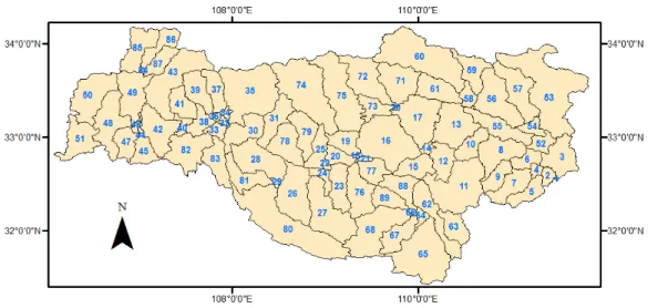
The upper Han river is divided into 89 sub-basins (REW-units). Each REW-unit has its own parameters and input data and is also assigned an ID-number. The ID-number is arranged so that the most downstream REW has the number one. From number one each REW is assigned a higher number the more upstream it is located. These numbers are unique and no REW has the same ID-number as another. The model is built using a digital elevation model (DEM) as a blueprint when estimating basin and sub-basin limits.
TsingHua Representative Elementary Watershed model (THREW)
Figure 4.5: The upper Han river basin divided into 89 REWs
Due to the climate in the upper Han river area (section 2.1) snow and glacial processes are excluded in this model.
No starting values for the hydrological situation are input into the upper Han river model. Instead, one year of simulation is used as warm up for the model.
Chapter 5
Data and methods
5.1
IMERG
The GPM precipitation product IMERG is readily available from NASA’s website. The data product provides precipitation data in a 0.1◦x0.1◦ grid for the whole globe and needs to be narrowed down to a rectangle that cover the upper Han river basin. This rectangle is defined by four corner locations in decimal degrees. The reference system used for the definition of location in degrees is the WGS 1984.
Table 5.1: Limiting corners for the GPM grid
Corner location Lon (Decimal Degrees) Lat (Decimal Degrees)
North West 106.05 34.25
North East 111.85 34.25
South West 106.05 31.35
South East 111.85 31.35
Data and methods
For a grid resolution of 0.1◦x0.1◦ the limiting rectangle contains a total of 1770 grid cells. Each cell that falls within a REW-unit will influence the rain input for the REW. The influence is calculated by dividing the area of the cell that intersects the REW with the total area of the REW. This influence is henceforth referred to as cell weight. Intersecting cells with REWs and calculating area of influence are performed using ArcGIS.
wj,k=
Aj,k
αk
(5.1)
wj,k : cell weight of GPM cell j for REW k
Aj,k : area of GPM cell j within REW k
αk: area of REW
Each precipitation input for REW k will thus be:
Pk: n
X
j=1
(wj,k·pj) (5.2)
Pk: input precipitation for REW k
pj : precipitation data of GPM cell j
All input data needs to have the same time resolution. Since the flow and gauge data is of an hourly resolution, it is unnecessary to have smaller time resolution on the GPM data. Therefore, the GPM data is converted into hourly averages (mm/hr) by arithmetic averaging.
GPM IMERG is provided in UTC time with no daylight savings adjustments. In order for the IMERG data to match the other model inputs temporally, it is converted to Beijing time (UTC+8). China does not use any daylight saving schemes and thus it is not required to adjust for any time changes during the year.
5.2
Rain gauges
Data and methods
Not all gauges are usable, some lack historical data, and some are faulty. The choosing criteria for the gauges were the following:
• Historical data has to exist between 2014-03-01 and 2016-03-01
• The data should not have too many missing values between above mentioned dates, i.e. lack historical data.
• The gauges have to fall within the basin limits.
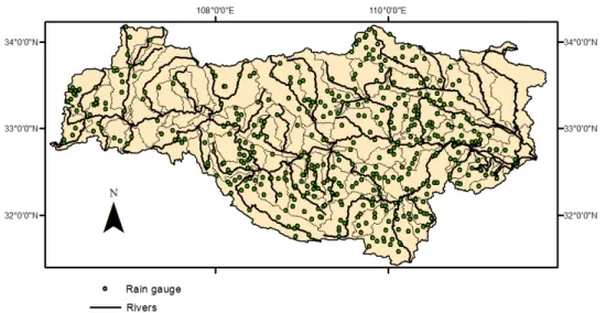
A gauge is defined as lacking historical data if there are no data for any of the months between 2014-03 to 2016-03. All the 2300 gauges are checked and sorted by an algorithm which applies the above criteria and sorts gauges in usable and non-usable. Out of these 2300 gauges, approximately 470 are considered usable after applying the sorting algorithm.
All of the gauges report in hourly accumulated precipitation in mm (mm/hr) with the minimum detection limit 0.2-0.5 mm/hr depending on gauge.
Figure 5.2: Usable gauges in the upper Han river
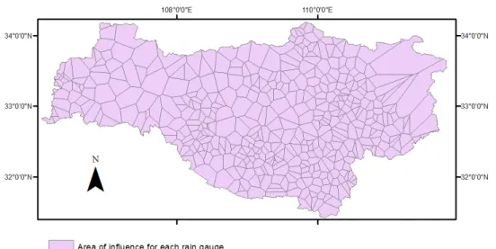
To convert gauge data into REW precipitation input, each gauge point is assigned an area of influence by creating Thiessen polygons. These polygons are then intersected with the REWs and influence factors are calculated as in section 3.1.1.
Data and methods
Figure 5.3: Area of influence using Thiessen polygons
5.3
Leaf area index
The model requires leaf area index as input for calculations of interception. The simplest way to attain this data is to download the MODIS-15 FPAR/LAI which is provided for free by NASA. The MODIS-15 comes with a global remote sensed 4- or 8-day composite of the leaf area index. It is provided in a grid based sinusoidal reference system with tiles of 10◦x10◦ around the equator. Each tile has a code as according to figure (5.4) and contains a raster with a spatial resolution of 1000m. [NASA, 2012]
Figure 5.4: MODIS 15 reference system [NASA, 2012]
For this project, the 4-day composite is chosen with the tiles h26v05 and h27v05. Since the data is a 4-day composite it is assumed that the LAI remains the same during all hours of these four days. Furthermore, the average of all tiles that intersects the
Data and methods
Figure 5.5: a) Example of a 4-day composite of leaf area index in the upper Han river
basin b)Resulting REW averaged LAI of a)
5.4
Reference evapotranspiration
China’s meteorological administration (CMA) operates four weather stations in the up-per Han river region. The meteorological data from these weather stations can be used to estimate the reference evapotranspiration with the Penman-Monteith equation. Ac-cording to ZHANG et al. [2012] the Penman-Moneteith is the most accurate method for estimating reference evapotranspiration in the whole Han river basin. The data from the weather station is provided as daily averages and thus the evapotranspiration can only be calculated into mm/day as the smallest time resolution.
Data and methods
Figure 5.6: Meteorological stations in the upper Han river region
The data that is provided by the CMA weather stations and its format can be found in the 5.2.
Table 5.2: CMA weather station data declaration
Data Data unit
Station number
-Year
-Month
-Day
-Average wind speed 0.1m/s Max wind speed 0.1m/s Direction of max wind speed direction Sunshine duration 0.1 hours Average air pressure 0.1 hPa Max air pressure 0.1 hPa Min air pressure 0.1 hPa Average temperature 0.1 C◦ Max temperature 0.1 C◦ Min temperature 0.1 C◦ Average water vapor pressure 0.1 hPa Average relative humidity 1% Min relative humidity 1%
To estimate the reference evapotranspiration, the FAO-56 empirically derived simplifi-cation of the Penman-Monteith equation was used. For the full calculation process and their corresponding equations see appendix (A) Since the net radiation at crop surface
dura-Data and methods
5.5
Discharge data
China’s hydrological bureau operates four river flow measuring stations in the basin. Danjiangkou, Baihe, Ankang and Yangxian. [Sun et al., 2014]
Figure 5.7: Hydrological stations on the upper Han river basin
Danjiangkou is located furthest down the river and at the final discharge of the whole basin. The water running into the Danjiangkou reservoir comes partially from upstream rivers that do not arise from mountainous areas. Thus the Danjiangkou hydrological station is not suitable to use. Baihe hydrological station is located upstream of Dan-jiangkou and covers mostly the mountainous areas of the upper Han river basin. For the purpose of modelling flash floods in mountainous areas, Baihe hydrological station is deemed to be the most appropriate to use.
5.6
Quantifying performance of the hydrological model
The performance of the hydrological model will be quantified by comparing simulated discharge to observed discharge using statistical indicators. These statistical indicators are the Nash-Sutcliffe coefficient (NSC) and index of volumetric fit(IVF).N SC= 1− PT t=1(Qtm−Qto)2 PT t=1(Qto−Q¯o)2 (5.3) IV F = ¯ Qm−Q¯o ¯ Qo (5.4)
Qtm: modeled discharge at time t
Qto: observed discharge at time t ¯
Data and methods
These statistical indicators will be applied for the whole period 2015-2016 but will also be concentrated for the flood period during summer. The flood period is defined as the time around the highest discharge peak in year 2015 to 2016.
Chapter 6
IMERG analysis and correction
6.1
Error analysis
Analysing differences between IMERG and gauges has to be done in order to better un-derstand the (lack of) performance of IMERG. It is assumed that rain gauges represent the true rainfall patterns. Henceforth are errors of IMERG defined as the difference be-tween IMERG data and rain gauge data. Both IMERG early and late run are analyzed at a grid level. Corrections are however applied at a REW scale to match input data format for THREW. For several gauges that fall within an IMERG cell, an arithmetic mean is used when comparing data. In order to quantify errors several statistical indica-tors will be used. Common statistical indicaindica-tors that are used in identifying errors are: root mean squared error (RMSE), mean bias (BIAS) and coefficient of determination (r2) [Chen and Li, 2016; Guoqiang et al., 2016; Rios Gaona et al., 2016].
RM SE= r Pn i=1( ˆyi−yi)2 n (6.1) BIAS = Pn i=1( ˆyi−yi) n (6.2) r2 = 1− P i(yi−yˆi)2 P i(yi−y¯)2 (6.3)
yi: observed value at point i
ˆ
yi: estimated value at point i
¯
y : mean observed value
IMERG analysis and correction
It is also of interest to analyse the accuracy of rain and dry events through a hit/miss matrix. To compare total rain volumes for period 2015-2016 between rain gauges and IMERG, data is interpolated from points to field using inverse distance weighting.
Z(x) = P wiZi P wi (6.4) Z(x) : interpolated value at x Zi: data point at i wi(x) = 1 d2 (6.5)
d: distance from point i to x
The total volume falling between April 2015 and March 2016 varies between 150 mm and 1500 mm over the basin. The southern part of upper Han river recieves most precipitation while there is a decline further north. Similarly for IMERG early and late both capture the total volume variation over the basin fairly well. IMERG early and late tend to overestimate in comparison to rain gauges with total volumes varying between 500 mm and 2200 mm. Heavy precipitation areas have a higher total volume in the late run than in the early run. The dry area in the northeast corner seems to be more concentrated for the late run than early run. Overall no version seems to be better at representing the spatial variation of the total volume in comparison to rain gauges than the other.
Looking at the total volume for rain gauges, it is uncertain whether some gauges may be faulty as their total volume differs considerably from the neighbouring gauges. To estimate how good IMERG is at detecting precipitation events a detection matrix is established. For each time step IMERG data and rain gauge network data are compared. If both IMERG and rain gauges record a rain event at the same time it is considered a hit. Similarly if both record no rain during the same time it is also considered a hit. If rain is recorded in the IMERG but not in the rain gauge it is considered as a false positive. If the opposite happens it is considered a false negative.
IMERG analysis and correction
Figure 6.1: The spatial variation of total precipitation volume for the period 2015 to
2016 for
a) gauges b) IMERG early(6h) c) IMERG late(18h)
Table 6.1: Detection accuracy of IMERG early and late to rain gauges, i.e. detection
matrix Gauge wet dry IMERG Early run wet 2.19 % 2.02 % dry 2.22 % 93.6 % Gauge wet dry IMERG Late run wet 2.40 % 1.98 % dry 2.00 % 93.62 %
as the lower limit, any detected precipitation below this limit is not included in the statistics.
The majority of all data points are dry events, i.e. no precipitation. It is clear that IMERG manages to detect the majority of all these dry events correct. For precipitation
IMERG analysis and correction
2% are correctly detected. IMERG has slightly more false negatives than false positives. The high amount of false positives and false negatives can be partially explained by low temporal accuracy. Possibly, the rain events that happen during a certain period might be detected at different times for different data sets. Guoqiang et al. [2016] show that the daily variation is not fully replicated in the IMERG final run, which means for early and late it should be even less.
As mentioned in section (3.3), previous research shows that errors in the IMERG are related to intensity and elevation. To further investigate these relationships each IMERG and gauge data point are compared at a grid scale. If more than one gauge falls within the IMERG cell, the average of the gauges will be used for comparison.
Applying the statistical indicators for the whole period gives a good understanding of how the errors are characterized.
IMERG analysis and correction
In figure (6.2 a-b) no clear correlation between errors and elevation can be found for neither the early run or the late run. Errors of IMERG seems to not be affected by small local elevation differences.
Both early run and late run have a clear overestimation of precipitation intensities over gauges which is shown in (figure 6.2 c-d) where data point clusters are skewered towards higher y-values. The late run seems to be just marginally better than the early run in estimating precipitation. However figures (6.2 c-d) also show that both IMERG early and late are overall very poor at estimating correct precipitation intensity.
Looking at the accumulated difference over time, two conclusions can be made. Firstly, IMERG tends mostly to overestimate but cases of underestimation exist as well. Sec-ondly, errors are not just attributed to temporal inaccuracy. If all errors were attributed to the temporal inaccuracy of IMERG the accumulated difference should tend to be zero over time, which is not shown in figures(6.2 e-f).The accumulated difference also shows that the errors increase mostly during the rainy periods, which further confirms that IMERG has an intensity estimation error.
Each statistical indicator is interpolated using inverse distance weighting over the whole basin to create a continuous field.
Table 6.2: Statistical indicators between rain gauges and IMERG
Early run Late run Min Max Min Max CC -21 0.35 -15 0.3 BIAS (%) -25 370 -19 410 RMSE (%) 730 4100 650 3500
Generally IMERG late run performs slightly better than the early run when looking at the statistical indicators. Forr2the early run has a span of -21 to 0.35 with an average of -1.9 while the late run has a span of -15 to 0.3 with an average of -1.8. The interpolated fields show that most agreement between IMERG and rain gauges happens around the dry northwest area of upper Han river. Most errors happens around a rain gauge that records relatively low total volume for the period in comparison to neighbouring gauges (fig. 6.3). Generally wetter areas show lower r2 in comparison to dryer areas for both IMERG early and late. Lower r2 in wetter areas could indicate that IMERG have problems for both intensity and temporal estimation errors.
The relative RMSE spans are 730% to 4100% for the early run while slightly lower for the late run ranging from 650% to 3500%. Theoretically, the temporal accuracy can
IMERG analysis and correction
Figure 6.3: Statistical indicators for IMERG early run and late run interpolated to a
continuous field over the upper Han river basin
by the satellite the calculated error would be pretty big even though the rain pattern matches well. In this case the big RMSE errors can be attributed to both temporal inaccuracy and intensity estimation inaccuracy.
IMERG analysis and correction
low or negative bias. Unlike the previous two indicators, mean bias is not affected by temporal inaccuracy since negative and positive values cancel each other.
6.2
Error correction
There are numerous methods and much research in correcting rainfall estimates. The errors in IMERG vary both spatially, temporally and with intensity, therefore a cor-rection method needs to account for these variables. Generally, corcor-rection requires an adjustment of the rainfall estimate to match a ’true’ data set, i.e. gauge measurements. The lack of research into IMERG correction means that correction methods for other satellite precipitation product will be used.
A method stemming from ground radar calibration, which is also used for satellite pre-cipitation estimates, is the multiplicative bias factor [Lia et al., 2017]. The process involves choosing a window for which a certain amount of time steps are aggregated. Both IMERG and gauges are aggregated for the same window and then adjusted through a multiplicative factor to match each other. The factors will be calculated in a grid-scale and then interpolated through Thiessen polygons to an area of influence over the basin. Further on, an average bias factor will be calculated for each REW (the same process as preparing precipitation input data).
Bhatti et al. [2016] showed that for CMORPH (a similar satellite rainfall product) the best results was 7-days backwards sequential window. This thesis will make use of Bhatti et al. [2016]’s results to correct IMERG.
BFiw = Pt=w t=d PiG(t) Pt=d+7 t=d PiI(t) (6.6)
BFiw : Bias factor for period w=d+7
PiG(t) : Precipitation of gauge i for time t
PiI(t) : Precipitation of IMERG i for time t
Pkcorr =Pkraw·BFk (6.7)
Pkcorr : corrected precipitation for REW k
Pkraw: uncorrected precipitation for REW k
Chapter 7
Results and Discussion
7.1
Upper Han river model results using rain gauge
pre-cipitation data as forcing
Running the upper Han river model with rain gauge precipitation data gives a good indication on how said model performs for 2015 . The rain gauge driven model acts as a baseline for which the performance of IMERG early (6h) and late (18h) runs can be compared against.
Results and Discussion
Table 7.1: Statistical indicators of the performance of rain-gauge driven hydrological
model in comparison to observed discharge data
Period NSC IVF
Whole 0.19 -0.06 Flood -0.10
-The gauge driven model has a fairly poor performance when looking at the NSC for the overall year. The poor overall performance can also be found in the discharge graphs (observed and simulated) in fig (7.1). The IVF shows that the total volume over the year between simulated and observed matches fairly well. The poor performance could possibly be explained by flow regulation in the upper Han river. Inflow into the Danjiangkou reservoir (reservoir at basin outlet) needs to be regulated for security purposes and thus there are numerous reservoirs that regulate the flow in the main river. Commonly reservoirs are also used for hydro power generation and thus flow regulation could also be influenced by power consumption and production.
Regulating reservoirs would mean that the river flow can be delayed and intensity re-duced in comparison to natural flow. The total runoff volume would still be similar over a long period for natural and regulated flow. The upper Han river model can only simulate natural flow in the basin, thus a low IVF suggests that the poor performance can be attributed to the target series showing regulated flow.
The regulation of stream flow is limited by reservoir capacity. Heavy floods can thus only be regulated to a certain extent. As shown in the discharge graphs the upper Han river model simulates the flood event in 2015 quite well. The first peak is overestimated but the second peak is very close. This can again possibly be explained by regulation. A theory is that the first flood is reduced by storing in the reservoirs but when the second wave of flooding arrives the reservoirs have already reached their regulating limit. This means that the first peak can be reduced while the second cannot. However, without certain knowledge on how regulation works in the upper Han river, this theory cannot be confirmed.
7.2
Performance of the hydrological model with IMERG
precipitation data
Both the uncalibrated and calibrated IMERG precipitation data has been run with the upper Han river model. Uncalibrated IMERG refers to the precipitation data set of IMERG that is not corrected with the bias multiplicative factor method, where as calibrated IMERG means that the method has been applied to it. The purpose of
Results and Discussion
IMERG with rain gauge data affects model results. Theoretically, if the rain gauge-driven upper Han river model does represent the natural flow (as opposed to regulated flow which discharge data might represent), IMERG should be compared to it as well.
Results and Discussion
Figure 7.3: Simulated discharge of uncalibrated IMERG early(6h) run and late (18h) run compared to rain gauge-simulated discharge
The uncalibrated IMERG has a clear overestimation of the flood event, which is both visible in the discharge graphs (fig. 7.2 and 7.3) and in the statistics (table 7.2) for the flood event. This result could be expected when looking at the error analysis for IMERG where the wet areas had relatively higher bias (50-100 percent). Such high overestimation might not be viable for flood predictions since even small flow peaks are greatly overestimated.
Table 7.2: Statistical indicators of the performance of IMERG driven hydrological model in comparison to observed discharge data
IMERG NSC IVF
Early -8.66 0.73 Late -10.91 0.88
There is a similarity between the simulated flow graphs of IMERG and gauges in terms of timing and shape. Since the IMERG early/late and rain gauges are independent of each other, the similarity further confirms the possibility of flow regulation in the discharge data.
Results and Discussion
Figure 7.4: Simulated discharge with calibrated IMERG precipitation data compared
Results and Discussion
Figure 7.5: Simulated discharge with calibrated IMERG precipitation data compared
to rain gauge-driven discharge simulation
The calibration of IMERG improves its performance vastly (fig. 7.4 and fig. 7.5). The total volume is heavily reduced and would possibly be viable in predicting floods. Worth noting is that the first flood peak is higher than the second peak, which is opposite to the rain gauge-driven upper Han river model. This can be due to different bias factors for the two corresponding periods. The peaks are split, coincidentally, in separate bias factor windows and may subsequently have different bias factors. Since the window is a 7-day accumulation, underestimation earlier in the window containing the first peak can have a reducing effect on the bias factor. This could affect the correction negatively.
Table 7.3: Statistical indicators on the comparison of simulated discharge driven by calibrated IMERG data with observed discharge and with rain gauge-driven discharge
simulation respectively
Comparison with Period IMERG Nash-sutcliffe IVF
Observed discharge
Whole Early -0.14 0.11 Late -0.21 0.16 Flood Early -1.51
-Late -1.22
-Rain gauge-driven discharge simulation
Whole Early 0.76 0.18
Late 0.75 0.24
-Results and Discussion
The IMERG early(6hr) run performs, after corrections, better than the corrected IMERG early(18hr) run overall (table 7.3). This result is a bit surprising since NASA states that the late run is more accurate than the early run. The IMERG early run performs better both compared against observed discharge and gauge-simulation. However when scaling down the statistical window to just the flood event, IMERG late performs significantly better. For an additional 12 hours delay the peak is estimated better in the late run. The lead time vs. accuracy needs to be considered when choosing the IMERG product.
7.3
Sources of errors
As with all models accurate input data is crucial in achieving good results. The uncer-tainties for each input data will add to the uncertainty of the simulation results.
7.3.1 Discharge data
One of the biggest uncertainties lies in the target series, i.e. discharge data. As dis-cussed in the earlier section, the discharge data may not be corrected for regulated flow which means that statistical indicators may not be representative for the model’s actual performance. Unreliable discharge data negatively affects the possibility to asses the errors in input data which will be explained in the corresponding subsection.
7.3.2 Rain gauge data
An equally important factor is the error in rain gauge precipitation data. In this project the rain gauges are considered to be the truth in depicting rainfall patterns. However, the rain gauges are not perfect in this representation. Each rain gauge can only measure the rainfall for a point in space, thus requiring interpolation when rainfall data for a continuous area is needed.
The interpolated data for certain areas might not reflect the spatial variation of the rainfall if the gauge density is low. This problem is reduced when the gauge density is high but can never be removed fully. For the upper Han river basin gauge density is fairly well but for some areas (such as north west) the density is lower and might lead to uncertainties when interpolating rainfall. Without the proper discharge data, however, assessing the rain gauge interpolation is difficult.
The rain gauge data from the provincial hydrological bureau is of varying quality, some rain gauges report every hour regardless of weather and some only report during rainfall events. The algorithm to sort out bad rain gauges works fairly well but, as discussed in section (6.1), some faulty gauges might have been included. This will affect the results
Results and Discussion
7.3.3 Reference evapotranspiration
There are only four meteorological stations in the upper Han river basin. Similar to rain gauges each measurement is discrete and needs to be interpolated to cover the whole basin. With only four measurement stations, the interpolated evapotranspiration is subject to more spatially related errors than the rain gauges. The temporal resolution of the measurements are daily averages and thus the diurnal variation cannot be repre-sented. This can give a slight impact on the model results since more evapotranspiration happens during the day than night.
As explained in section (5.4) the data from the meteorological stations are not direct measurements of evapotranspiration but rather parameters that affect it. The FAO 56 Penman-Monteith is a empirical method to derive the reference evapotranspiration from these parameters. This means that to obtain the most accurate results, empirical coefficients need to be calibrated.
There are no calibration data available for the upper Han river basin (as of 2016) and thus recommended values are applied (as mentioned in section 5.4). Without calibration, reference evapotranspiration is most likely to differ from actual reference evapotranspi-ration. However, this method is still deemed to be the most accurate one for the upper Han river basin.
7.4
IMERG correction method
This thesis makes use of a correction method commonly used when correcting ground radar against rain gauges. This method was evaluated for the satellite product CMORPH in the basin of Gigil Abbey in Ethiopia [Lia et al., 2017]. The findings of the aforemen-tioned evaluation are applied to this study. However, CMORPH is derived using different satellites and algorithms. The window scale and movement used for CMORPH might not be the most effective one for IMERG. As no such equivalent evaluation of optimal window scales and movement for IMERG has been made (as of 2016), using CMORPH findings was the best choice.
The error correction relies on rain gauges and thus more rain gauges should give a better error correction. There are two ways in creating a continuous bias correction field. Either an interpolated rain gauge field is compared to the IMERG field or the bias factor for each IMERG cell that contains rain gauges is interpolated. Both ways add uncertainties onto the final correction field and determining which one would be most suitable can only be done by trail and error.
Results and Discussion
7.5
Interpolation methods
The main method for interpolating input data is the Thiessen polygon method. When interpolating rainfall, more accurate interpolating methods exist such as, kriging. Simi-larly, when interpolating bias factor more advanced interpolation methods (such as in-verse distance weighting ) can be used as well. These methods are more complicated and requires more time to execute. The simplicity of Thiessen polygon reduces the amount of work needed. For high density rain gauge networks Thiessen polygons should produce acceptable results. With sparser data points however, more sophisticated interpolation methods should be considered
Chapter 8
Conclusion
8.1
Using IMERG for flood prediction
This study has made use of a high density rain gauge network to analyze the potential of the near real-time satellite IMERG products as input data when forecasting flash floods. The IMERG product is far less accurate than the rain gauge network for both flood prediction and overall flow prediction. The gauged precipitation data performed at N SC = 0.2 overall and N SC = −0.1 for peak flow period, while the IMERG un-calibrated data performed at N SC = −8.66 (early) and N SC = −10.91 (late) overall and N SC =−66 (early) andN SC =−77 (late) for peak flow period. The correlation between IMERG and rain gauges was found to be poor (avg. r2=−1.8 for IMERG late andr2=−1.9 for IMERG early ), with some areas showing as high asr2= 0.2 (IMERG late) andr2 = 0.35 (IMERG early) while others as low asr2 =−15 (IMERG late) and
r2 = −21 (IMERG early). The combination of gauge precipitation data and IMERG precipitation data showed a remarkable improvement for hydrological model results but still not on par with using only the rain gauge-data.
In conclusion, the results of ths study show that IMERG has a potential for flood forecasting but good results rely on rain gauge assisted correction. The IMERG product by itself is not viable at this stage for flood prediction.
8.2
Further research
As mentioned in the previous section, the gauge network used in this study had a reasonably high density. For real flood forecasting applications, further research should be done on IMERG correction and performance in areas with low gauge density. Ideally a basin with relatively few rain gauges where heavy flooding occurs should be chosen. The discharge data needs to reflect natural flow or a model that can simulate regulated flow
Appendices
the corresponding low density rain gauge network in flood forecasting can be decided. Since there is not a lot of research into rain gauge-correction methods for IMERG, further investigation of it should also be done. Further research can also be done for the multiplicative bias factor method such as optimal window size and movement.
Appendix A
FAO 56 Penman-Montieth
calculation process
ET0 = 0.408∆(Rn−G) +γT900+273u2(es−ea) ∆ +γ(1 + 0.34u2) (A.1)ET0 : reference evapotranspiration (mm/day)
Rn= net radiation at crop surface (MJ/(m2 day))
G= soil heat flux (MJ/(m2 day))
T = air temperature at 2 m height (C*)
u2 = wind speed at 2 m height (m/s)
es= saturation vapour pressure (kPa)
ea= actual vapour pressure (kPa)
∆ = slope vapour pressure curve(kP a/C∗)
γ = psychometric constant (kPa/C)
∆ = 4098(0.6108e 17.27T T+237.3) (T+ 237.3)2 (A.2) γ = 0.665P ·10−3 (A.3) eo(T ) +eo(T )
FAO 56 Penman-Montieth calculation process
eo= 0.6108eT17+273.27T.3 (A.5)
Rn=Rns−Rnl (A.6)
Rns= net solar radiation
Rnl = net outgoing long wave radiation
Rns= (1−α)Rs (A.7)
α= 0.23(albedo for hypothetical grass crop)
Rs = incoming solar radiation (MJ/(m2 day))
Rs= (as+bs
n
N)Ra (A.8)
n= sunshine duration [hours]
N = maximum possible sunshine duration [hours]
Ra= extra terrestrial radiation [M J/(m2·day)]
Ra=
24·60
π Gscdr(ωssinϕsinδ+ cos$cosδsinωs) (A.9)
Gsc= solar constant = 0.0820M J/(m2·min)
dr = inverse relative distance between earth and the sun
ωs= sunset hour angle [rad]
ϕ= latitude of measuring station
δ= solar decimation
dr = 1 + 0.033 cos(
2π
FAO 56 Penman-Montieth calculation process
J = current day out of L in the year [day]
L= length of year [days]
ωs= arccos(−tanϕtanδ) (A.12)
Rnl =σ (Tmax,K)4+ (Tmax,K)4 2 ·(0.34−0.14√ea)· 1.35Rs Rso −0.35 (A.13) σ: Boltzmann’s constant) = 4.903·10−9
Tmax,K : maximum temperature a certain day [K]
Tmin,K : minimum temperature a certain day [K]
ea: actual vapor pressure [kPa]
Rs: the incoming solar radiation
Rso: clear sky solar radiation
For non-calibrated as and bs:
Rso=Ra(0.75 + 2·10−5z) (A.14)
References
Allen, R. G., Pereira, L. S., Raes, D., Smith, M. et al. [1998], ‘Crop
evapotranspiration-guidelines for computing crop water requirements-fao irrigation and drainage paper 56’,FAO, Rome300(9), D05109.
Aon-Benfield [2016], ‘Global catastrophe recap’. Accessed 2016-08-24.
URL: http://thoughtleadership.aonbenfield.com/Documents/20160908-ab-analytics-if-august-global-recap.pdf
Bhatti, H. A., Rientjes, T., Haile, A. T., Habib, E. and Verhoef, W. [2016], ‘Evaluation of bias correction method for satellite-based rainfall data’, Sensors16(6).
URL: http://www.mdpi.com/1424-8220/16/6/884
Britannica, E. [2016], ‘Huang he floods’. Accessed 2016-08-19.
URL: https://www.britannica.com/event/Huang-He-floods
Chen, F. and Li, X. [2016], ‘Evaluation of imerg and trmm 3b43 monthly precipitation products over mainland china’,Remote Sensing8(6), 472.
Guoqiang, T., Yingzhao, M., Di, L., Lingzhi, Z. and Yang, H. [2016], ‘Evaluation of gpm day-1 imerg and tmpa version-7 legacy products over mainland china at multiple spatiotemporal scales’, Journal of Hydrology533(1), 152–167.
Huffman, G., Bolvin, D., Braithwaite, D., Hsu, K., Joyce, R., Kidd, C., Nelkin, E. and Xie, P. [2015], ‘Nasa global precipitation measurement (gpm) integrated
multi-satellite retrievals for gpm (imerg) version 4.5’.
URL:
https://pmm.nasa.gov/sites/default/files/documentfiles/IM ERG AT BD V4.6.pdf
Lia, N., Tang, G., Zhao, P., Hong, Y., Goue, Y. and Yang, K. [2017], ‘Statistical assessment and hydrological utility of the latest multi-satellite precipitation analysis imerg in ganjiang river basin’, Atmospheric Research183(1), 212–223.
References
NASA [2011b], ‘Gpm data downloads’. Accessed 2016-08-26.
URL: https://pmm.nasa.gov/data-access/downloads/gpm
NASA [2012],MODIS LAI/FPAR Product User’s Guide.
NASA [2017], ‘Global precipitation measurement (gpm)’. Accessed 2016-08-24.
URL: https://pmm.nasa.gov/image-gallery/gpm-constellation-1-31-2017
NSSL [2016], ‘Severe weather 101’. Accessed 2016-08-25.
URL: http://www.nssl.noaa.gov/education/svrwx101/floods/
Rios Gaona, M. F., Overeem, A., Leijnse, H. and Uijlenhoet, R. [2016], First-year evaluation of IMERG - Final Run in the Netherlands, in ‘EGU General Assembly Conference Abstracts’, Vol. 18 of EGU General Assembly Conference Abstracts, p. 16683.
Sun, Y., Tian, F., Yang, L. and Hu, H. [2014], ‘Exploring the spatial variability of contributions from climate variation and change in catchment properties to streamflow decrease in a mesoscale basin by three different methods’, Journal of Hydrology 508, 170–180.
Tian, F., Hu, H. and Lei, Z. [2008], ‘Thermodynamic watershed hydrological model: Constitutive relationship’,Science in China Series E: Technological Sciences
51(9), 1353–1369.
URL: http://dx.doi.org/10.1007/s11431-008-0147-
![Figure 3.1: The GPM satellite constellation [NASA, 2017]](https://thumb-us.123doks.com/thumbv2/123dok_us/499052.2558958/19.893.234.711.130.523/figure-the-gpm-satellite-constellation-nasa.webp)