Theses and Dissertations Graduate School 2015
Graph-based Regularization in Machine Learning: Discovering
Graph-based Regularization in Machine Learning: Discovering
Driver Modules in Biological Networks
Driver Modules in Biological Networks
Xi GaoFollow this and additional works at: https://scholarscompass.vcu.edu/etd
Part of the Artificial Intelligence and Robotics Commons, Bioinformatics Commons, Microarrays Commons, Systems Biology Commons, and the Theory and Algorithms Commons
© The Author Downloaded from Downloaded from
https://scholarscompass.vcu.edu/etd/3942
This Dissertation is brought to you for free and open access by the Graduate School at VCU Scholars Compass. It has been accepted for inclusion in Theses and Dissertations by an authorized administrator of VCU Scholars Compass. For more information, please contact [email protected].
A dissertation submitted in partial fulfillment of the requirements for the degree of Doctor of Philosophy at Virginia Commonwealth University
by
Xi Gao
Master of Science in Bioinformatics from Virginia Commonwealth University, 2010 Bachelor of Science in Medicine from Sun Yat Sen University, 2008
Director: Dr. Tomasz Arodz
Assistant Professor, Department of Computer Science
Virginia Commonwealth University Richmond, Virginia
1 Introduction 1
1.1 Motivation . . . 1
1.2 Contributions of the Dissertation . . . 3
1.3 Structure of the Dissertation . . . 5
2 Background 7 2.1 Biological Networks . . . 7
2.2 Differential Analysis of Gene Expression . . . 8
2.2.1 Differential Co-expression . . . 9
2.2.2 Gene Set Enrichment Analysis . . . 10
2.2.3 Differential Sub-network Detection . . . 10
2.3 Machine Learning . . . 12
2.3.1 Basic Terms . . . 12
2.3.2 Algorithm Types . . . 13
2.3.3 Supervised Learning Algorithms . . . 14
2.3.4 Regularization in Supervised Learning . . . 16
3 Evaluation of Supervised Machine Learning Methods 19 3.1 Evaluation Scheme . . . 19
3.1.1 Cross-validation Framework . . . 20
3.1.2 Performance Evaluation . . . 21
3.2 Benchmark Non-biological Datasets . . . 23
3.2.1 Gaussian Dataset . . . 23
3.2.2 Time Series Dataset . . . 23
3.2.3 Image Analysis Dataset . . . 24
3.3 Simulated Biological Datasets . . . 25
3.3.1 Motivation for Simulating Biological Datasets . . . 25
3.3.2 Dataset Simulation Framework . . . 26
3.3.3 Base Network Extraction . . . 27
3.3.3.1 GeneNetWeaver Simulation Theory . . . 27
3.3.3.2 Modeling Different Phenotypes . . . 29
3.3.4 Simulated Datasets used in Experiments . . . 30
3.3.4.1 PhosphoFull Network Dataset . . . 30
3.3.4.2 Phospho200 Network Dataset . . . 31
4.2 Proposed Method for Graph Connectivity Constrained AdaBoost . . . 36
4.2.1 Connectivity-deletion AdaBoost . . . 37
4.2.2 Connectivity Penalty Module . . . 38
4.2.3 Deletion Function . . . 40
4.2.3.1 Tree-based Deletion with Enforced Connectivity . . . 40
4.2.3.2 Feature-based Deletion with Enforced Connectivity . . . 41
4.2.4 Model Retraining . . . 42
4.3 Computational Complexity . . . 43
4.4 Results and Discussion . . . 45
4.4.1 Phospho200 Dataset . . . 47
4.4.2 Phospho200 Mutation Dataset . . . 50
4.4.3 PhosphoFull Dataset . . . 52
5 Linear Support Vector Machine with Submodular Graph Regularization 54 5.1 Background . . . 54
5.1.1 Linear Programming Support Vector Machine . . . 54
5.1.2 Submodular Functions and their Convex Extensions . . . 56
5.2 Proposed Method for Submodular Graph-based Regularization in Linear SVM 60 5.2.1 Graph-based Regularization in SVM . . . 60
5.3 Results and Discussion . . . 62
5.3.1 Biological Datasets . . . 62
5.3.2 Benchmark Non-biological Datasets . . . 64
6 Boosting with Proximal Descent and Submodular Graph Regularization 66 6.1 Background . . . 66
6.1.1 AdaBoost as a Descent Method in Functional Space . . . 66
6.1.2 Boosting as a Descent Method in the Space of Real Vectors . . . 71
6.1.3 Proximal Gradient Descent . . . 73
6.2 Proposed Method for Submodular Graph Regularization in Boosting . . . 76
6.3 Results and Discussion . . . 82
7 Conclusions 85
3.1 Confusion Matrix . . . 21
3.2 PhosphoNetwork Edges with Modified Dissociation Constant . . . 31
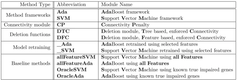
4.1 Abbreviations of Module Names . . . 46
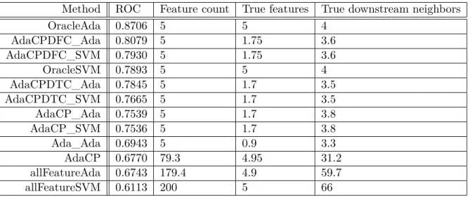
4.2 Results for Phospho200 Dataset . . . 48
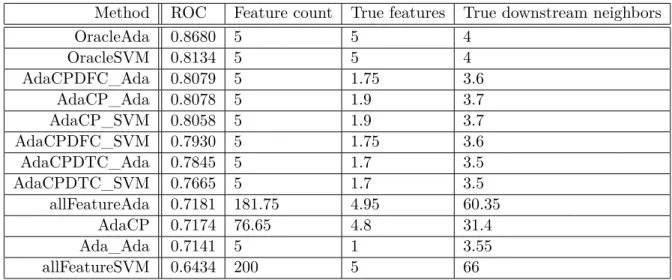
4.3 Results for Phospho200 Mutation Dataset . . . 51
4.4 Results for PhosphoFull Dataset . . . 52
5.1 Linear SVM results for Phospho200 Dataset . . . 63
5.2 Linear SVM results for PhosphoFull Dataset . . . 63
5.3 Linear SVM results for Phospho200 Mutation Dataset . . . 63
5.4 Linear SVM results for Gaussian Red Dataset . . . 64
5.5 Linear SVM results for Gaussian Cyan Dataset . . . 64
5.6 Linear SVM results for Gaussian Green Dataset . . . 64
5.7 Linear SVM results for time series Dataset . . . 65
5.8 Linear SVM results for MNIST Dataset . . . 65
6.1 Boosting results for Phospho200 Dataset . . . 83
6.2 Boosting results for PhosphoFull Dataset . . . 83
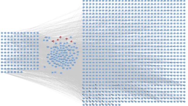
3.1 Gaussian dataset and its feature network - a random graph with 100 nodes. . . 24 3.2 Complete view of PhosphoFull network. Edges marked red between diamond
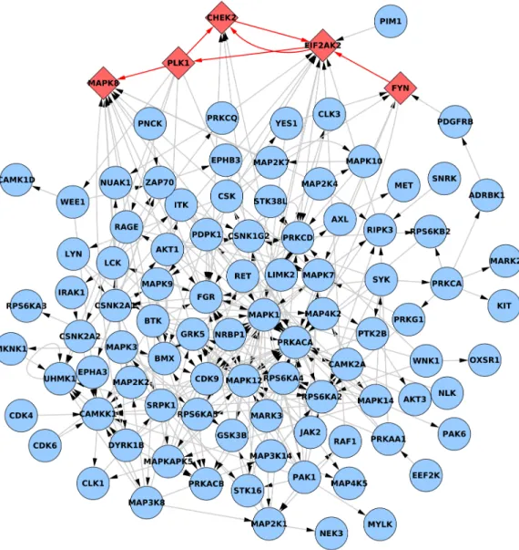
red nodes are impaired. Dissociation constants of impaired edges are increased thirty times for pathological phenotype data simulation. Left grid contains nodes that have null in-degree while right grid groups nodes with no outbound edges. . . 32 3.3 Core of the PhosphoFull network after removing nodes with null in- or
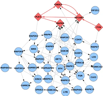
out-degree. Edges marked red between diamond red nodes are impaired. Disso-ciation constants of impaired edges are increased thirty times for pathological phenotype data simulation. . . 33 3.4 Phospho200 network extracted from full PhosphoNetwork. Edges marked red
between diamond red nodes are impaired. Dissociation constants of impaired edges are increased two times for pathological phenotype data simulation. Left grid contains nodes that have null in-degree while right grid groups nodes with no outbound edges. . . 34 3.5 Core of the Phospho200 network after removing nodes with null in- or
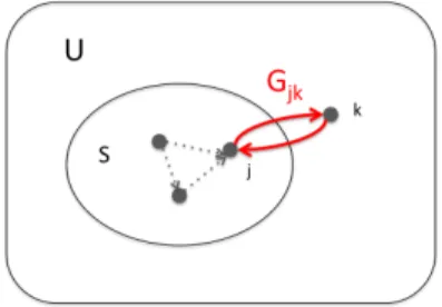
out-degree. Edges marked red between diamond red nodes are impaired. Disso-ciation constants of impaired edges are increased two times for pathological phenotype data simulation. . . 34 5.1 Graph cut regularizer penalizes undirected edges that cross setS boundary. . . 57
5.2 Graph cut regularizer penalizes directed edges that cross setS boundary. . . . 57
5.3 By adding elementx, a smaller set Areceives bigger increase of edge numbers that cross the expanded set boundary than a larger set B. U represents the universe of set elements, equal to the set of graph vertices V. . . 58 5.4 Graph cut set function and its values for a single specific edge are defined at
points (0,0), (0,1), (1,0), (1,1). We assume Gjk = 1 in the plot. . . 59
5.5 Lovasz extention of the graph cut submodular function is convex, piece-wise linear, and equal to the original submodular set function at the corners of the unit hypercube, (0,0), (0,1), (1,0), (1,1). We assume Gjk = 1 in the plot. . . 60
1 Cross-validation Label Generation . . . 20
2 Cross-validation Framework . . . 21
3 Data Simulation Pipeline . . . 27
4 Subnetwork Extraction for Simulation . . . 27
5 AdaBoost Algorithm . . . 36
6 AdaCPDFC/AdaCPDTC - Connectivity-deletion AdaBoost . . . 38
7 Connectivity Penalty Module . . . 39
8 Tree-based Deletion with enforced Connectivity (DTC) . . . 41
9 Feature-based Deletion with enforced Connectivity (DFC) . . . 42
Discovering Driver Modules in Biological Networks
by
Xi Gao
A dissertation submitted in partial fulfillment of the requirements for the degree of Doctor of Philosophy at Virginia Commonwealth University
Virginia Commonwealth University, 2015
Director: Dr. Tomasz Arodz, Department of Computer Science
Curiosity of human nature drives us to explore the origins of what makes each of us differ-ent. From ancient legends and mythology, Mendel’s law, Punnett square to modern genetic research, we carry on this old but eternal question. Thanks to technological revolution, to-day’s scientists try to answer this question using easily measurable gene expression and other profiling data. However, the exploration can easily get lost in the data of growing volume, di-mension, noise and complexity. This dissertation is aimed at developing new machine learning methods that take data from different classes as input, augment them with knowledge of fea-ture relationships, and train classification models that serve two goals: 1) class prediction for previously unseen samples; 2) knowledge discovery of the underlying causes of class differences. Application of our methods in genetic studies can help scientist take advantage of existing biological networks, generate diagnosis with higher accuracy, and discover the driver networks behind the differences. We proposed three new graph-based regularization algorithms. Graph Connectivity Constrained AdaBoost algorithm combines a connectivity module, a deletion function, and a model retraining procedure with the AdaBoost classifier. Graph-regularized Linear Programming Support Vector Machine integrates penalty term based on submodular graph cut function into linear classifier’s objective function. Proximal Graph LogisticBoost adds lasso and graph-based penalties into logistic risk function of an ensemble classifier. Re-sults of tests of our models on simulated biological datasets show that the proposed methods are able to produce accurate, sparse classifiers, and can help discover true genetic differences between phenotypes.
Introduction
1.1 Motivation
In the past two decades, techniques for exploration of biological systems grew swiftly. Gene expression profile measurement became easier, faster and cheaper. Array-based methods such as DNA microarrays and sequence-based techniques like RNA-seq are taking the main stage in biological and medical experiments. Other techniques that operate at genetic, epigenetic, transcriptomic, proteomic and metabolomic level are also in rapid progress. In result, sci-entists can capture global snapshots of thousands gene expression levels of many patients. Increasingly, they are also able to place them in the context of gene mutations, promoter methylation, chromatin states, protein abundances, and lipid profiles.
Rapidly growing volumes of experimental data are full of promise, but snapshots with so many variables pose a challenge – they are no longer easily interpretable. Results from profiling experiments are increasingly easy to obtain, but become notoriously hard to process and understand. The purposes of gene expression and other profiling analyses is to formulate novel and plausible hypotheses to narrow down possible new knowledge of studied objects, such as the explanations of a certain disease. Then, further detailed experiments focusing on narrowed list of targets should be performed to confirm the hypotheses. However, due to the scale, noise and complexity of profiling data, formulating reasonable hypotheses becomes a major bottleneck.
bi-ological research. Concepts from biology inspired many machine learning algorithms such as artificial neural network, likewise the broad application of machine learning algorithms benefits many biology fields, especially genetic research. By their nature, machine learning algorithms learn from existing data to derive models for prediction, classification and pattern recognition. This facilitates the process of hypotheses generation and reasoning about molec-ular mechanisms in many areas of genetic research, including high-throughput gene expression analysis. In unsupervised studies, clustering algorithms group genes or patients based on the distances calculated from the expression matrix. In supervised studies, classification models with high prediction accuracy can serve as diagnostic or prognostic rules. Compact models with selected small number of variables, or features, can help scientists narrow down from countless possible hypotheses to a selected few, and raise evidence to illustrate the underlying basis of the molecular differences between phenotypes.
Despite many advances, traditional machine learning algorithms struggle with forming models that are accurate, interpretable and concise when faced with highly-dimensional pro-filing data. One reason is that classification methods based on statistical learning are purely data-driven. They do not use existing knowledge when they analyze the data. They miss on the rapidly growing domain knowledge related to genetic research – gene ontologies, gene regulatory interactions, protein-protein interactions. Many databases with useful information are available online and a large number of them are organized in the form of biological net-work. Can machine learning algorithms be designed to comprehend domain knowledge and use it for analyzing gene expression data? Can such new algorithms improve classification performances? Driven by these questions, we steered our research towards designing algo-rithms for incorporating domain knowledge in the form of biological networks into machine learning methods in a way that leads to classification models with improved accuracy and interpretability.
There is an abundant knowledge of gene regulatory and protein-protein interactions, but what are the potential benefits of using biological networks in model training? First, in su-pervised machine learning, selecting informative features for training is the key to building successful models. The immense number of features in the analysis of gene profiles makes many learning methods lose power. The nature of graph-based biological networks illustrate
the relationships between genes - these relationships reveal closeness and dependency between features, and can counter the effects of statistical noise inherent in datasets with small number of samples. Combined with methods from graph theory, these feature-to-feature relationships could be used in feature grouping, extraction and selection. For example, grouping of genes into sets, based on pathways in a network or other information, resulted in the move from univariate analysis to gene set enrichment analysis. In machine learning, we could use fea-ture relationships as a source of constraints on models, to guide training and optimization. Second, previous domain knowledge could help rationalize experiment design. Gene expres-sion analysis used to focus on single gene expresexpres-sion variation between phenotypes. However, when genetic research provide more gene regulation information in terms of network, many researchers start differential co-expression analysis [28, 29, 60] that leads to fruitful result. Third, models built from biological networks are easier to interpret. In univariate gene differ-ential expression analysis or traditional supervised feature selection studies, multiple single selected genes leave scientists no biological mechanism to follow up on, but network-guided expression analysis select significant changed gene subnetworks or pathways to be explored further. Fourth, limiting the models to subnetworks can lead to simpler models. What are the potential benefits of choosing simpler classifiers? Simple models mean shorter testing time, so given the same accuracy, simpler models are more efficient. Also, simple models are less prone to overfitting. Furthermore, as we stated before, smaller connected models are easier to interpret biologically.
1.2 Contributions of the Dissertation
In this study we propose three method for constructing classifiers that predict the phenotype of samples. Even though many state-of-art methodologies including machine learning intend to construct systems to mine out the differences between phenotypes through gene expression, there is shortage of methods that build high-accuracy classifiers that can facilitate biology elucidation.
Our first method is Graph Connectivity Constrained AdaBoost. By adding network nectivity constraint, deletion function and model retraining procedure to Adaboost, we
con-structed a new supervised machine learning classification algorithm. We tested our method on simulated data with known differences between classes. Our proposed method shows higher predicting accuracy, flexibility and interpretability than state-of-the-art methods. Our second method is Graph Regularized Linear SVM. By adding graph regularization term in to linear SVM objective function, we encourage linear SVM to select features that organize small highly internally connected independent subnetworks. We test our graph regularized linear SVM with other linear SVM methods on three biology datasets and three non-biology datasets. Results show our Graph Regularized Linear SVM method outperform other linear SVM methods. Our third method is Proximal Graph LogisticBoost. We modify the risk func-tion of LogisticBoost by adding convex extension of submodular graph cut set funcfunc-tion and integrating it into boosting through proximal gradient descent. Proximal graph LogisticBoost highly improved the performance of AdaBoost and LogisticBoost in biological datasets.
In summary, the major contributions of the research are
1. We integrated biological network knowledge with machine learning algorithms for gene expression analysis.
2. We proposed three new graph-based supervised classification methods that has been shown to:
(a) predict sample classes with high accuracy; (b) produce sparse classifiers;
(c) discover the true genetic differences between different phenotypes.
3. We improved performance of AdaBoost with our Graph Connectivity Constrained Ad-aBoost by including:
(a) network connectivity penalty module; (b) deletion function;
(c) variable importance feature selection model retraining procedure.
4. We improved performance of linear SVMs with our Graph Regularized Linear SVM by including:
(a) graph regularization term into SVM objective function;
5. We improved boosting with our Proximal Graph LogisticBoost by including: (a) graph regularization term into logistic risk function;
(b) lasso regularization term into logistic risk function;
6. More generally, we demonstrated how to incorporate nonlinear, non-differentiable penalty terms, e.g. those based on submodular set functions, into boosting.
1.3 Structure of the Dissertation
The rest of this dissertation is organized in the following way. In Chapter 2 we review the background relevant to our research. Specifically, in Section 2.1 we explore major types and sources of biological networks. In Section 2.2 we go through the major challenges of gene expression analysis and summarize the state-of-the-art methods that approach the problem from different angles. In Section 2.3 we recapitulate basic knowledge of machine learning that is the foundation of our research.
In Chapter 3, we introduce the experimental framework and the datasets we will use in evaluating the proposed methods in subsequent chapters. In Section 3.1 we explain the cross-validation setup we used. Also, we introduce the metrics that measure the performance of classification methods. In Section 3.2 and Section 3.3, we describe three non-biological datasets and three biological datasets we used for evaluating our methods.
In Chapter 4 we introduce a new machine learning classification algorithm we developed for solving the problem of graph-based learning. We introduce classical AdaBoost algorithm that our algorithm is based on in Section 4.1. Then, in Section 4.2 we describe the design of the new algorithm, Graph Connectivity Constrained AdaBoost, and the details of the connec-tivity penalty module, deletion function and the model retraining procedure. Connecconnec-tivity module integrates biological network knowledge into model training, while deletion function and retraining procedure lead to smaller classifiers of higher accuracy. We analyze our method and show their performance in Sections 4.3 and 4.4.
In Chapter 5, we introduce graph regularization in linear SVM. In Section 5.1 we introduce linear SVM and the convex extensions of submodular functions that will form the basis for the graph regularization. In Section 5.2, we propose our Graph Regularized Linear SVM method. In Section 5.3 we present results of our proposed method along with other linear SVM methods.
In Chapter 6, we introduce our submodular graph regularized boosting method. We explain boosting theory in the perspective of gradient descent in Section 6.1. We elaborate on details of the new Proximal Graph LogisticBoost algorithm in Section 6.2. Then we compare the new graph-based boosting method results along with state-of-art results in Section 6.3.
Finally, in Chapter 7, we summarize the conclusions from our current solutions to the problem of classification and finding differentially expressed modules in biological networks.
Background
Our work is focused on differential analysis of molecular profiles, such as gene expression data, by using machine learning methods, and by extending them with knowledge of biological networks. In this Chapter, we provide background information about these three focus areas.
2.1 Biological Networks
Graph is a data structure broadly used to represent objects as well as their relationships. Biological objects such as genes and proteins organized in a graph form a biological network. In bioinformatics, this typically includes gene regulatory networks, protein-protein interaction networks, signaling pathway networks or metabolic networks. Depending on the type of the interactions, these networks can be classified as a directed or undirected graphs. As the knowledge of biochemistry and molecular biology accumulates, biological networks become more and more complex. Large, comprehensive networks with large number of nodes and edges provide scientists opportunities, but also challenges. How to efficiently store and organize these networks and mine out the hidden biological information behind the labyrinthine graphs are two major issues. Various databases are built for biological networks and many existing and new graph algorithms have been used in conjunction with these networks to answer biological questions.
Here we review two major biological networks we have been using in our research -BioGRID and PhosphoNetworks. -BioGRID is a public database that contains
comprehen-sive information on genetic and protein-protein interactions collected from multiple sources for human and other model organisms [49]. It was first created in 2003 and it is continu-ously updated [44]. There are 217,928 human genetic and physical interactions in total in the 2013 version of BioGRID network we downloaded. Most BioGRID network interactions are gathered from literature studies, and the experimental method used for discovering the inter-action is recorded in BioGRID along the interinter-actions. A study based on Bayesian learning showed differences in confidence that can be assigned to interactions discovered by different experimental system [58]. This difference in confidence of evidence is presented as probability scores, where higher score means higher confidence in the evidence behind the interaction.
Another biological network we used is focused on a subset of protein-protein interactions. PhosphoNetworks is a public biological network database that focuses on human kinase-substrate phosphorylation relationships [22, 23, 38]. Rather than being collected from lit-erature, all the interactions stored in PhosphoNetworks are validated by proteomic-based strategy. Phosphorylation reactions of 289 human kinases on 4,191 human proteins are tested and 3,656 phosphorylation relationships are identified and stored in the database.
2.2 Di
ff
erential Analysis of Gene Expression
As genome-wide expression profiles became more available, computational methods aimed at discovering differences between two or more phenotypes entered into a rapid development phase to deal with the newly available breadth of data. Because of the relatively small sample size and large feature space of genome-wide expression data, traditional univariate analysis based on comparison of means or correlation with class variable showed multiple disadvantages:
1. low statistical power resulting from ignoring the fact that groups of genes act together in a biological function and mild change of expression level of each gene could result in significant cell malfunction or hyper-function that leads to phenotype differences. Treating genes independently reduces the ability to identify genes that act as a set but with non-significant expression level changes by themselves;
correction for large number of variables;
3. if some genes are identified as significant, there is often little overlap of genes in exper-iments conducted by independent groups;
4. identified genes cannot tell us much about the biological processes and pathways involved in the studied pathology.
Various categories of methods are designed to overcome these disadvantages of traditional univariate methods. Below, we review the major current solutions for the above problems. 2.2.1 Differential Co-expression
Differential co-expression analysis is gaining attention in recent years as a tool for finding phe-notypic differences that are more complex than univariate differences. The approach aims at detecting pairs of genes that show differences in gene regulation and cellular signaling between two phenotypes. Differential co-expression brings a new perspective on differences between phenotypes – that a specific phenotype could result from differences in gene regulation that do not significantly alter average expression levels of genes, but alter the pattern of behavior of the genes in tandem. For example, expression levels of a pair of genes may be tightly correlated in one phenotype, where one of the genes regulates the other, but uncorrelated in another phenotype, where the regulation is lost due to mutation or other reasons. This idea has been proven true in a lot of biological conditions such as obesity [52], aging [48] and cancer [57].
Existing differential co-expression detection methods usually measure some gene pair re-lationship score separately in each phenotype condition, then compare the difference of these scores. The score most often used is the Pearson correlation coefficient, applied in conjunction with Fisher’s Z transformation [7, 61] that yields a probability distribution of the differences in correlation. However, Pearson correlation coefficient is highly affected by outlying samples. Efforts to make correlation more resilient to outliers were undertaken by using biweight mid-correlation [25]. Rank-based and entropy-based measurements [31], as well as F-statistic [29] are also used. In terms of the number of gene as a unit in the differential co-expression network, some methods aim at gene pairs while others aim at gene modules [28,40,60].
2.2.2 Gene Set Enrichment Analysis
Gene Set Enrichment Analysis (GSEA) [50] is designed to improve the disadvantages of tra-ditional statistical methods. GSEA takes genes in a pre-defined gene set as a group and uses it to assess the results of univariate tests. In effect, GSEA translates results from the level of independent genes to a level of pre-defined, biologically meaningful sets of genes. These pre-defined gene sets could be derived from existing biological knowledge. Genes acting to-gether in the same cellular process or same signaling pathway could be grouped toto-gether. For example, known oncology genes could be defined as a group. By doing this, genes functioning as a group could be tested together, revealing the cellular function changes associated with disease phenotypes. Based on the list of genes sorted according to the correlation between their expression levels and sample classes obtained from a statistical test, GSEA defines an enrichment score. GSEA operates by going through the sorted list of genes, increasing a score for each gene from the pre-defined set and decreasing it for genes from outside the set. The increment is proportional to the correlation between the gene’s expression level and the sample class, so if genes from the set are concentrated at the top or at the bottom of the list, the GSEA score will be far from null. Significance level of the enrichment score is calculated by permuting genes and adjusted for multiple hypotheses testing using false discovery rate (FDR). GSEA was originally validated on leukemia and lung cancer data sets and the results showed the method is able to discovery strong significant gene sets while univariate analysis find little significant gene and no overlap between repeat experiments [50].
Gene set enrichment analysis, even though it overcomes a lot of disadvantages of traditional univariate analysis, has its limitations. It only tests genes in a set together as a whole but fails to take the topology of inter-gene relationships into consideration. Moreover, as it is only based on pre-defined gene sets, it has no power to discover new gene sets that differentiate biological phenotypes.
2.2.3 Differential Sub-network Detection
Based on observed data, can we tell which genes changed expression as a group under different experimental conditions and what are the signaling pathways connecting these genes? In order
to move beyond pre-defined pathways employed in gene set enrichment analyses and be able to answer questions like this, research in computational biology started to focus on methods for detecting active modules under certain experiment conditions. Ideker and his team was the first one who started to tackle this problem [24]. They first build up a statistical scoring system for sub-networks to detect how much the expression level of such sub-network changed under certain condition. Then, using simulated annealing, they search the full network to find the sub-network with the optimal score heuristically. After obtaining high-scoring sub-networks of genes, they used Fisher’s exact test and random walk approach to determine statistical significance of discovered sub-networks. Cytoscape, a commonly used software in network biology, employed this sub-network searching algorithm as a plug-in, ActiveModules, and it has been applied in many biological domains, such as diabetes [32]. The ActiveModules sub-network searching algorithm has been extended by combining it with differential co-expression method, thus replacing genes by gene interactions as the input [17]. Rather than picking up the sub-network of genes, the methods intends to pick up the sub-network of gene-interactions that changed most under experiment conditions. Pearson correlation coefficient is used to represent the edge scores of pairs of genes, and again simulated annealing is used to pick up the optimal sub-network of gene edges with the most statistically significant accumulated edge score.
Chuang et al. [8] used a greedy approach for gene sub-network discovery and applied it in breast cancer metastasis research. In their algorithm, they give an activity score to each gene sub-network by averaging gene expressions of such sub-network. Then they calculate mutual information of activity score of each sub-network and sample classes. They take each single gene as a seed, and grow corresponding sub-network using such seed greedily. Sub-network with local maximum mutual information score will finally be chosen.
Most gene sub-network detection methods try to search for connected gene groups that, in aggregate, exhibit statistically significant differential expression. Another approach to this problem is to use an additive score for the group, based on the univariate scores of individual genes. Then, the task is to find a connected component from a graph that maximizes the score. With non-negative scores, the maximum is the whole graph, so a penalty is used to limit the size of the discovered subnetwork. If the penalty is assigned to each edge in the
subnetwork, the optimal solution is a spanning tree, known as the prize-collecting Steiner tree. Steiner tree problem is NP-hard and has been studied extensively [11, 27, 36, 59]. Based on Dreyfus-Wagner algorithm [11], Scott et al. [46] developed their Steiner tree algorithm to pick up meaningful gene sub-network. They calculate p-values of differential expression for each gene and used ≠log(1≠p) as prize for each gene. Based on a known gene network structure
and user-defined gene prizes, their algorithm could pick up the sub-network that represents regulatory pathway altered under experimental condition. Bailly-Bechet et al. approached the sub-network detection problem the same way with an improved solver for the Steiner tree problem [2].
2.3 Machine Learning
Many of the most successful methods for analyzing data coming from biological experiments involve machine learning. Machine learning is an important discipline in computer science. It emerged from early artificial intelligence field and touches many different fields of science and industry, such as biology, neuroscience, image processing, robotics and language processing. The main task of machine learning is to learn, recognize and predict patterns from data. By applying machine learning algorithms, we turn raw records into new knowledge. Arhur Samuel defined machine learning in 1959 as a “Field of study that gives computers the ability to learn without being explicitly programmed”. This points to the generalization ability of machine learning algorithms. A good framework of supervised machine learning algorithm should be autonomous. Given training data and domain knowledge, algorithms should be able to derive model for future prediction by integrating information without human interference. 2.3.1 Basic Terms
In our study we focus on supervised learning algorithms. In supervised machine learning, featuresare individual measurable properties or attributes that have been recorded;samples are individual objects whose features have been recorded; classes are the labels of samples that indicate their categories. Well-behaved features, samples and sample classes are crucial to the success of machine learning algorithms. Good features are supposed to be discriminative
and independent. That means there is little overlapped information or association between features. In practice, this ideal is rarely reached. This opens the opportunity for our proposed graph-based regularization methods, which make use of known relationships between features captured in a form of a graph. Some examples of features are age, gender, p53 expression value. Good samples are supposed to be independent and identically distributed. That means first there is little association between samples; second all samples of the same class should be polled from the same population. The number of classes should be small compared to the number of samples. Often, machine learning algorithms are designed for problems where only two classes are present. Such binary sample classes are usually represented by 1/0 or 1/-1. For example class label 1 represent healthy people and class label -1 represent cancer patients. In our study all classes are labeled in 1/-1.
2.3.2 Algorithm Types
Depending on the types of their input and output data, machine learning algorithms could be organized into four major fields - supervised learning, unsupervised learning, semi-supervised learning and reinforcement learning. Insupervised learning, the training data always come in pairs with data labels - we know the correct answers to sample classes. Supervised learning algorithms take samples values and sample classes as input, learn the associations between them in training stage, then try to predict sample classes for new sample values in testing stage based on the learned associations. The most popular supervised learning algorithms today are Support Vector Machine (SVM), Artificial Neural Network (ANN), decision tree and ensemble learning (bagging, boosting and random forest).
In unsupervised learning, there is no label for any sample, so there is no training and testing stages as in supervised learning. Unsupervised learning algorithms aim at recognizing the patterns and inner structure of data. For example,clustering algorithmsgroup samples based on their closeness to each other, while association rules extract abstract rules of objects’ relationships from inventory of object sets. Semi-supervised learning is situated between supervised and unsupervised learning. Usually semi-supervised learning data are comprised of large amount of unlabeled and small amount of labeled data.
learning algorithms try to learn from previous actions that lead to punishments or rewards so that algorithms’ future actions maximize cumulative rewards. It is widely studied in disciplines like game theory, control theory, and operations research. Reinforcement learning models are composed of 1) a set of environment states S, 2) a set of actions A, 3) rules of transitioning between states, 4) rules that determine the scalar immediate rewards of a transition, 5) rules that describe what the agent observes. An example of reinforcement learning application is an autopilot system. We set environment states as different road systems, a set of actions as move forward, backward, or turn, rules to transitioning between different road systems, rules that determine punishments and rewards for wrong or correct operations and rules that describe observed results.
2.3.3 Supervised Learning Algorithms
Our research is focused on supervised learning algorithms. Supervised methods can be cat-egorized based on the properties of data labels. If the data labels an algorithm takes and produces are both continuous, then the algorithm is a regression algorithm; otherwise, if the data labels are discrete categorical numbers (usually binarized as 1/0 or 1/-1), then the algorithm is aclassification algorithm. We focus here on classification algorithms, so below we provide a brief review of the most popular supervised learning algorithms commonly used in classification analysis.
Support Vector Machine (SVM)in its modern form was published in 1995 by Vladimir
N. Vapnik and Corinna Cortes [9]. In training phase, SVM looks for a hyperplane that maximizes the margin between two classes of samples. Those samples lying on the margin are called support vectors. Kernel trick in SVM maps samples onto a high-dimensional space that leads to efficient non-linear classification. Soft margin SVM allows for accepting samples lying on the wrong sides of the margin, rendering higher generalization power and limiting overtraining. SVM can be reformulated for regression analysis too. More details about the basic, linear version of SVM will be presented in Chapter 5.1.1.
Artificial Neural Network (ANN)is comprised of input, output and optional hidden
layers of nodes that are interconnected between layers. To train an ANN we feed the data through the input layer through hidden layers and collect result from the output layer. By
comparing results with sample labels, we calculate errors and correct weights on connections between nodes. Eventually, when all weights converge, a trained neural network system is able to predict sample classes with high accuracy. But ANN is a black box model and its weights are hard to interpret. The first model of ANN was introduced in 1943 [35]. It was once a very popular research topic until 1969, when Marvin Minsky and Seymour Papert’s publication put the research into stagnation [37]. They revealed two problems about ANN - single layer neural networks cannot solve “exclusive-or problem”; and multi-layered networks with linear nodes can be reduced to single layer networks. The backpropagation algorithm [43,54] and an ANN model with nonlinear nodes in hidden layers successfully solved the “exclusive-or problem” and neural network regained attention. Even though in the 1990s SVM and other new machine learning methods such as ensemble learning reduced popularity of neural networks, recent research in deep learning [20] resulted in another explosion of interest in the field.
Decision Tree uses a tree-like structure as the classification model. All the training
samples pass through the root node, and are directed towards the leaves by decisions at each node. Each node of the tree contains a split based on a threshold of a selected feature. The split guides the samples that reached the node into the node’s left and right child. Each of the leaves of the tree indicates a single class to be assigned to samples that reach the leaf. In the training stage we train a decision tree, typically in a greedy fashion, and in the testing stage decision tree could predict sample classes by letting samples go from the root through splits to leaves. Decision tree is not a black box model so it is simpler to understand and interpret. However, as it is not resistant to overfitting and is highly susceptible to noise in the training set, usually decision tree cannot get results with high accuracy in complicated data sets. On the other hand, due to its low computational complexity and inherent instability, decision trees are commonly used as base classifiers in ensemble learning (bagging, random forest, boosting).
Decision Stump is a very simple type of decision tree, in which the tree has just one
level. That is, we predict one class for all samples that have the value of the feature higher than the threshold, and the other class for all samples for which the value of the feature is below the threshold. Which feature is the deciding feature, what is the threshold, and which class is above the threshold and which is below is decided based on the training data. We
chose one feature, one split or threshold on that feature, and the orientation of that split, in a way that minimizes the classification error on the training set.
Ensemble classifiersaggregate multiple learning models to predict results. This highly
enhances the prediction accuracy and model resistance to overfitting. Major ensemble methods are bagging, random forest and boosting. Bagging is also called bootstrap aggregating. It was proposed by Leo Breiman in 1996 [4]. The idea of bagging is to create multiple training sets of the same size by random sampling with replacement from original training set. Models are built upon those new training sets and final prediction is the average of predictions of all the models. Random forest [6, 10] is the application of bagging technique in feature spaces. In addition to sampling samples as in bagging, random forest sample features for multiple model training. Boosting is another ensemble classifier that is superficially similar to bagging, with the added weights of base models, and weights of points that focus training on samples that are hard to classify, typically because they are close to the decision boundary separating the classes. However, it has a deeper interpretation as an iterative method for optimizing the risk of the classifier. Our work is based on extending boosting to improve its accuracy on biological datasets, and we discuss boosting separately in more detail in Sections 4.1.1, 6.1.1 and 6.1.2.
2.3.4 Regularization in Supervised Learning
Classification algorithms such as those described above extract models by learning from train-ing samples data and their categories. Then, the trained model, or a classifier, is used to pre-dict unknown categories for new data samples. Classifiers should generalize well to previously unseen samples, and should also be parsimonious and interpretable.
Many classification problems involve a feature space that is very highly dimensional. For example, in biological classification problems, the number of experimental genes or proteins are almost always much larger than the number of patients. As a result, the density of training samples in the feature space is very low, which may result in overfitting. Overfitting happens when classifiers describe training data too well, and they lose their robustness and generalization ability. Thus, overfitted classifiers usually perform poorly in prediction and are unstable to noise fluctuation. When feature dimensions are much higher than training
sample sizes, classifiers are usually overly complex. Complex classifiers that contain excessive number of parameters are often overfitted.
Various methods were invented to deal with overfitting and regularization is one of the most important class of techniques. Regularization aims to limit overfitting by penalizing model complexity. L1 and L2 regularization are classic regularization paradigms that were initialy used in regression, but are also used in classification.
L2 regularization adds L2 norm of parameter weights into loss function to control model complexity. For example, in a linear model, the sum of squares of weights of features in the model would be incorporated into the loss function. Ridge regression [21] is a statistical application of L2 regularization. Classical linear SVM is another example. However, L2 regularization’s feature weight decay effect cannot effectively reduce feature numbers, since penalty drops very quickly as feature weights approach zero, and there’s little incentive to actually reach null feature weight and eliminate the feature from the model completely. As a result, classical linear SVM classifiers can still contain many parameters with small weights.
To obtain more parsimonious classifiers, feature selection methods such as recursive feature elimination [19] are usually combined with SVM. These external feature selection methods are called wrapper. They rank features by their importance and remove less important features to reduce feature size. By testing numerous feature sizes, wrappers choose the best feature subset for model training. Wrappers are very computational expensive and unstable due to its greedy disposition [18]. One would desire a regularization method with embedded feature selection property that does feature selection and model construction simultaneously. L1 regularization can accomplish such effect by driving some feature weights to zero. This leads to sparse models that are preferred [39]. LASSO [51] and LARS [14] are example of statistical methods involvingL1 regularization. Zou and Hastie proposed Elastic net regularization [64] that combines L1 and L2 penalty parts. The L1 penalty part contributes to the sparsity of models andL2 penalty partially releasesL1from its feature selection limitations. Additionally, L2 penalty part promotes a grouping effect that encourages selection of related features as a group.
The methods described above are all purely data-driven. Besides experimental data, domain knowledge is helpful to model success. For example, in genetic study, gene groupings
or interactions established through decades of biology experiments can play an important role in illuminating new studies. In image processing, neighboring pixels are often similar, with variation that can be attributed more to noise than to the actual difference. In recent years, group LASSO was introduced to incorporate additional information about groups formed by features. Also, pre-defined quadratic spatial kernels over features were used to improve image processing using AdaBoost [56]. Quadratic penalties on graphs were also proposed for linear regression [30].
Evaluation of Supervised Machine
Learning Methods
In this Chapter we describe how the methods we propose in this dissertation will be evaluated. This includes the description of performance metrics and the validation procedures. We also present the datasets that will be used for evaluating the methods, and propose our own method for creating realistic, simulated biological two-class datasets.
3.1 Evaluation Scheme
To evaluate supervised learning algorithms, we usually partition samples into training and testing parts. We feed algorithms training samples and their classes as input, and let algo-rithms learn a model that recognizes the patterns in the data. Then we can generate predicted classes for testing samples using the model learned from training samples and classes. By com-paring the predicted test sample classes to the known true test sample classes, we evaluate the algorithm’s performance on test data. The most common problem in supervised machine learning algorithms is overfitting. It is also called overtraining. In supervised machine learning it means the learning algorithms selects too complicated models to fit training data accurately so that the models fit to noise and loose generalization power to predict future data accurately. The opposite side of overfitting isunderfitting. It is also calledundertraining. Underfitting means machine learning algorithms select too simple models to fit training data.
In the situation of underfitting, models have equally low predicting power over both training and testing samples.
Cross-validation is mainly used in supervised learning and it is a useful technique to avoid overfitting. It partitions experiment samples into several different parts called “folds” (e.g. five-fold cross validation partitions samples into five parts). In classification problems, each part is supposed to have the same proportion of samples from each class. Cross validation chooses one part of the partitions as “testing set” while the rest serve as “training set”. Machine learning algorithms extract models from training sets in “training stage” and predict on testing sets in “testing stage”. We could evaluate algorithms by checking their average performance on all different cross-validation training/testing sets derived from given dataset. 3.1.1 Cross-validation Framework
For testing the methods, we store and use the same cross-validation labels for a given dataset. When we use cross validation to test the method performances on a dataset, we have to avoid using different cross-validation partitions of data for different methods, because different data partition introduce noise to the estimate of the method’s performance. We generate and save 10 independent five-fold cross validation labels for each dataset as specified in Algorithm 1. We then test methods for any given dataset using cross-validation labels generated as specified in Algorithm 2. We go through five-fold cross validation of this data set when testing performances of methods. For each method, we average the results of those 50 runs. Algorithm 1 Cross-validation Label Generation
foreach datasetddo forj Ωrun{1, ...,10} do for iΩclass{1,≠1} do Si= (sampleœclass); SÕi=P ermute(S); for kΩ{1, ..., m}do label(SÕ i(k)) = 1 + (k mod 5); end for label(SÕ
i,sort) = sortlabel(SiÕ) according to Index(Si);
end for
save five-fold cross validation label(Ssort) for jth run of datadto file asSd,j.
end for end for
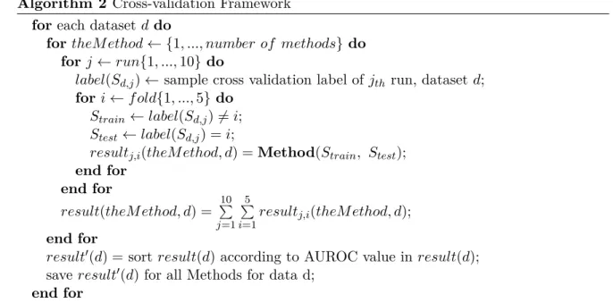
Algorithm 2 Cross-validation Framework for each datasetddo
for theM ethodΩ{1, ..., number of methods} do
forjΩrun{1, ...,10} do
label(Sd,j)Ωsample cross validation label ofjth run, dataset d;
foriΩf old{1, ...,5}do
Strain Ωlabel(Sd,j)”=i;
Stest Ωlabel(Sd,j) =i;
resultj,i(theM ethod, d) =Method(Strain, Stest);
end for end for result(theM ethod, d) = q10 j=1 5 q i=1
resultj,i(theM ethod, d);
end for
resultÕ(d) = sortresult(d) according to AUROC value inresult(d); save resultÕ(d) for all Methods for data d;
end for
Given a dataset, we compare the average results of all methods and sort them by their mean AUROC value, which we introduce below in Section 3.1.2. Experiment results are presented in the result and discussion section by the end of each method chapter.
3.1.2 Performance Evaluation
There are many ways to measure the performance of an algorithm. In supervised learning, we assume we know the true label of some test samples so that we could evaluate our algorithm by comparing the predicted values of labels for testing samples to the true ones. A table called confusion matrix or contingency table (Table 3.1) shows different possible scenarios.
True positives (TP) and true negatives (TN) are correctly classified testing samples. False negative (FN) is rejection error, also called type I error. False negatives are true positive samples that are predicted negative. False positive (FP) is acceptance error, also called type II error. False positives are true negative samples that are predicted positive. From the
Table 3.1: Confusion Matrix
XXXXXXXX XXX
Truth Prediction Positive Negative Total
Positive True Positive (TP) False Negative (FN) P Negative False Positive (FP) True Negative (TN) N
contents of the confusion matrix, we can calculate a set of values that are often used to measure the quality of predictions generated by supervised classification machine learning algorithms.
Sensitivityis also called recall. It means how often the algorithm finds out true positive samples. It is an estimate probability that a true positive sample will be predicted correctly.
Sensitivity =T P/P =T P/(T P +F N) (3.1)
Specificitymeans how often the algorithm finds true negative samples. It is an estimated probability that a true negative sample will be predicted correctly.
Specif icity=T N/N =T N/(F P +T N) (3.2)
Accuracy means how often the algorithm finds true sample labels. It is an estimated probability that a sample will be predicted correctly.
Accuracy = (T P +T N)/(P+N) (3.3)
Precision means how often the predicted positive samples are truly positive. It is an estimated confidence of a predicted positive sample.
P recision=T P/(T P +F P) (3.4)
False positive rate (FP rate) means how often the true negative samples are falsely predicted positive.
F P rate=F P/N =F P/(F P +T N) = 1≠Specif icity (3.5)
False Discovery rate (FDR)means how often the predicted positive samples are falsely predicted.
Receiver Operating Characteristics Curve (ROC curve) is used to analyze per-formance of binary classifiers that return a continuous decision that is later converted into a binary prediction using a threshold. ROC curve is a smooth line connecting dots plotted in the space of FP rate and sensitivity. Each dot represents the value of FP rate and sensitivity of tested algorithm at a given threshold for classification. Area under the ROC curve (AUC or AUROC) equals to the probability that the classifier will differentiate a randomly cho-sen true positive from a random chocho-sen true negative sample. Its power is equivalent to the Wilcoxon/Mann-Whitney U rank test.
3.2 Benchmark Non-biological Datasets
While our work is focused on biological network and data, we have identified three datasets from outside of the biological field, as a way to show the generality of our methods.
3.2.1 Gaussian Dataset
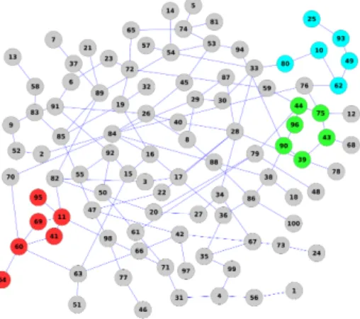
We have created an artificial, toy dataset with the size small enough to all be convenient during algorithm development. The dataset has 10000 samples and 100 features, connected by a random graph depicted in Fig 3.1. In the graph, three small connected subgraphs of different topology are identified, labeled as red, green and cyan. We created three datasets corresponding to these three colors. In each dataset features corresponding to one of the three subgraphs are the discriminative features. All other features are Gaussian random noise.
We tested Heuristic Graph AdaBoost and Graph Regularized Linear SVM on three dif-ferent Gaussian datasets. We used five fold nested cross validation for parameter tuning and testing results.
3.2.2 Time Series Dataset
We have used a real-world time series datasets with 121 samples and 637 features. The dataset describes a two-class problem of differentiating two types of atmospheric lightnings, based on features that describe electromagnetic power density of the atmosphere measured from a satellite in regular time intervals in the sub-microsecond range. The series of such
measurements together forms a time series that describes a single lightning event.
In classical classifier training using e.g. SVM or boosting, the information that the features correspond to consecutive time points would be lost. To show how graph-based regularization can help in time series data, we have constructed a graph in which each feature is connected to the feature representing the previous time step. We have used the graph as an additional knowledge in graph-based regularization.
We tested Heuristic Graph AdaBoost and Graph Regularized Linear SVM on time series datasets. We used five fold nested cross validation for parameter tuning and testing results. 3.2.3 Image Analysis Dataset
Our next dataset is incorporated to demonstrate how graph-based regularization can help with image analysis. The NIST (National Institute of Standards and Technology) handwrit-ten digits database that contains Special Database 1 which is sampled from American Census Bureau employees and Special Database 3 which is sampled from American high school stu-dents. NIST is a hard dataset for image processing as its training (Special Database 1) and testing (Special Database 3) samples are from different population. Each image of a digit contains 28 by 28 pixels, that is, 784 features. MNIST (Mixed National Institute of Stan-dards and Technology) handwritten digits dataset mixed Special Database 1 and 3 from NIST dataset. It then split the mixed samples into training set of 60,000 images and testing set of 10,000 images. MNIST is, compare to NIST, an easier dataset for image processing, and is widely used for machine learning method testing, including our tests in this dissertation. We
have used the pixels in the images as features, and we constructed a regularizing graph by treating each pixel as a vertex, and adding an edge between adjacent pixels. That is, a pixel is connected to it’s top, bottom, left and right neighbor.
We tested Heuristic Graph AdaBoost and Graph Regularized Linear SVM on three dif-ferent Gaussian datasets. We used five fold cross validation for parameter tuning on MNIST training dataset. Then we tested methods on MNIST test set using parameter chosen from previous step.
3.3 Simulated Biological Datasets
We tested Heuristic Graph AdaBoost, Graph Regularized Linear SVM and Proximal Ad-aBoost on biological datasets. For testing Graph Regularized Linear SVM, we used five fold nested cross validation for parameter tuning and testing results. For Heuristic Graph Ad-aBoost, we used 10 replicates of two fold cross validation for parameter tuning and testing results. For Proximal AdaBoost, we used five fold cross validation to choose optimal param-eters then test on ONE test set.
3.3.1 Motivation for Simulating Biological Datasets
Our research is dedicated to developing new algorithms that detect the underlying differ-ences between phenotypes using gene expression data and gene network information. Gene expression profiles with different phenotypes are organized in a matrix of feature values for each sample and a vector of class labels. Each column of the matrix is a gene acting as a feature while each row is a sample, typically corresponding to a patient. Every sample has a corresponding class label 1 or -1 to indicate which phenotype group it belongs to. Gene network is organized in adjacency matrix that indicates the relationships between features.
The two major tasks of the new algorithms are to 1) obtain models from training data and matching networks to predict classes for previously unseen samples, given sample gene expression profile; 2) extract the hypotheses of underlying differences between two phenotypes from the model. Performance of algorithms with respect to the first task can be assessed using methods such as cross-validation. However, validating the performance of algorithms on the
second task is problematic: 1) the true underneath network structures of gene regulation and protein interactions are unknown; 2) the true differences between two phenotypes are unknown. Even though gene expression profiles and network information for real life datasets are widely available, there is only limited information about the causes of differences between phenotypes. Moreover, most available human biological networks are incomplete maps of the genetic interactions. Results of algorithms integrating these incomplete networks with complete genetic expression information are not completely valid or comparable. For the purpose of algorithm development and evaluation, data simulation becomes our best option.
3.3.2 Dataset Simulation Framework
Proper experiment datasets should have gene expression values of two classes from the same network structure. Sample values of class one are generated from the intact network, while sample values of class two are from the network with selected regulation or signaling damage. The regulation damage is achieved by altering the dissociation constant k of corresponding edges. Dissociation constant kof edge AæB specifies strength of regulation of B byA.
To shorten testing time, we started with networks of limited size but with preserved basic regulation pathways. We extracted desired networks from existing high confidence biological network PhosphoNetworks [23] for simulation. The network extraction details are explained in Subsection 3.3.3, Algorithm 4. All selected impaired edges are connected. We modify dissociation constantkbased on network size and type of impairment. Molecular and experimental noises are added to all simulated datasets. Normalization procedure is applied to all noised datasets. We use GeneNetWeaver software [45] to simulate two sample classes of gene expression profiles. The GeneNetWeaver simulation model are illustrated in Subsection 3.3.3.1 and the datasets we obtained from the simulations are described in subsection 3.3.4. Machine learning method performance evaluation criteria are listed in Section 3.1.2. In our research, we use area under the ROC (receiver operating characteristic) curve as the final metric to evaluate all method we test. The complete pipeline for data simulation and method evaluation is outlined in Algorithm 3.
Algorithm 3 Data Simulation Pipeline choose a base network N;
datanormΩ GeneNetWeaver simulation from N;
define impaired network Nimpaired with chosen impaired edgesEimpairedfrom N;
dissociation constant kÕ(Eimpaired) =x·k(Eimpaired);
dataimpairedΩ GeneNetWeaver simulation fromNimpaired withk;
d=union(datanorm, dataimpaired)
result(d) =crossValidation(data)
Algorithm 4 Subnetwork Extraction for Simulation Require: : 1) A biological network Gwithm nodes.
2) Node size nof desired subnetworkGÕ. Selectp the longest of all shortest paths in G; for iΩgenes{1, ..., m}do
di = the distance of nodeitop;
end for
VÕ Ω sort all the verticesV = (v1, v2, ..., vm) in Gby corresponding D= (d1, d2, ..., dm);
select the top nnodes from VÕ;
GÕ Ω edgesEÕ inGwith both nodes inVÕ. 3.3.3 Base Network Extraction
The first step of simulation is to extract a well-structured network of desired size. The ex-tracted networks should preserve some biological pathways and other network properties. Net-work structures generated from random graph models such as Watts-Strogatz model (small-wold), Barabási–Albert model (scale-free) and Erd s–Rényi model (independent edges) do not capture statistically overrepresented biological network properties such as modularity and net-work motifs occurrences [42, 47]. Applying raw existing subnetnet-work extraction methods will break pathways and render graph-based machine learning methods irrelevant. For example, sub-networks of PhosphoNetworks generated from random extraction by GeneNetWeaver have longest path of only 3 edges. Networks for our experiment preferably should have at least one complete long signaling pathway with other pathways growing along it. To achieve this task, we designed an extraction method shown below in Algorithm 4.
3.3.3.1 GeneNetWeaver Simulation Theory
GeneNetWeaver (GNW) [45] is an open-source software for in silico simulation of gene ex-pression data based on an underlying gene regulatory network. Originally it was designed
to evaluate network inference methods. Theory behind the simulation model is described in [33] and we summarize it here because it is needed to explain our way of creating different phenotypes.
Expression value simulations are based on a network structure. Given a network, for each gene i, GNW simulates FiRN A, the change rate of mRNA concentration, andFiP rot, the change rate of protein concentration. Functionfi(·) serves as the activation function ranging
from 0 to 1 representing the relative activation of gene i. Furthermore, mi is the maximum
transcription rate, ri is the translation rate, ⁄RN Ai and ⁄P roti are the mRNA and protein
degradation rates andx,yare vectors containing all mRNA and protein concentration levels, respectively. The dynamical model is
FiRN A(x,y) = dxi dt =mi·fi(y)≠⁄ RN A i ·xi (3.7) FiP rot(x,y) = dyi dt =ri·xi≠⁄ P rot i ·yi (3.8)
Random fluctuations and molecular noise in transcription and translation process are modeled be changing a dynamic model of the form
dXt dt =V(Xt)≠D(Xt) (3.9) into a model dXt dt =V(Xt)≠D(Xt) +c 3Ò V(Xt)÷v+ Ò D(Xt)÷d 4 , (3.10)
where V(Xt) is the RNA or protein production; D(Xt) is the degradation; ÷v and ÷d are
independent Gaussian noise processes; and c is a constant to control the amplitude of the noise.
The relationships between a transcription-factor (TF)j and genei(j æi) is modeled by the probability of states of gene i. State S1 means TF j is bound to the promoter region of gene i while state S0 means not bound. The probability of TF j and gene ibinding P{S1}
promoter region, and onnij, the Hill coefficient. The probability can be expressed as P{S1}= ‰j 1 +‰j with ‰j = A yj kij Bnij . (3.11)
If –0 is the relative activation for state S0 and –1 the relative activation for state S1, given P{S1}, we could derive P{S0} as its complement, and define the function describing mean activation of gene igiven the concentrationyj of TF j:
f(yj)i=–0P{S0}+–1P{S1}=
–0+–1‰j
1 +‰j (3.12)
In real biological network, the interaction relationships are more complicated than one to one: one gene could be controlled by N TFs. With each TF possibly bound or not bound to such gene, we will have 2N states in total. Thus the function describing mean activation of genei
given concentrations y of its N regulators could be calculated as f(y) =
2N≠1 ÿ
m=0
–mP{Sm} (3.13)
Here is an example how to calculate the activation a gene that is regulated by two TFs: f(y1, y2) = –0+–1v1+–2v2+–3flv1v2
1 +v1+v2+flv1v2 with vj = (yj/kj)
nj (3.14)
3.3.3.2 Modeling Different Phenotypes
For testing our methods, we need datasets that contain samples from two different phenotypes. To generate such datasets, we need to simulate sample expression values for two phenotypes separately. We first use GNW to simulate normal samples with selected network structure. We choose stochastic simulation with multifactorial molecular and experimental noise added. GNW software will set all simulation parameters automatically. Along with the normal sample expression values, we get a normal network model with parameters from GNW. We create a pathological network model by modifying dissociation constantsk of the selected impaired edges and keeping other parameters intact. We feed back this pathological network model to GNW software and it will generate the pathological sample expression values. By doing
this, we could ensure samples from both classes come from the same network structure with the same other simulation parameters and same amount of noise added. The only differences are the dissociation constants of impaired edges. We treat these edges and their incident vertices as the “true differences” between two phenotypes. As we can tell from equation 3.11, the modification of dissociation constant kij of the simulation model changes the regulation
strength of TF j over gene i. By altering dissociation constants of selected edges, multiple related gene regulation relationships are impaired in simulated pathological situation.
We applied such modeling procedure to two different network structures - PhosphoFull and Phospho200 network. Because PhosphoFull network has 4375 edges while Phospho200 network has only 591 edges, we increase dissociation constants of the same set of impaired edges 30 times in PhosphoFull network while 2 times in Phospho200 network. To simulate gene mutations of the same pathway, we used a similar modeling procedure on Phospho200 network, but instead of impairing all edges in our predefined set, we create five different mutation models for five different impaired edges from the same set. Each mutation model contains the same set of parameters as the normal network model but with one edge dissociation constant increased 10 times. We simulate one fifth of pathological samples using each mutation model and put these samples together as a whole pathological expression set. This mutation dataset is called Phospho200 Mutation. It models the real-world situation where pathology is based on alteration of a single pathway, but in individual patients different components of that pathway are altered. All datasets are described in details in subsection 3.3.4.
3.3.4 Simulated Datasets used in Experiments 3.3.4.1 PhosphoFull Network Dataset
PhosphoFull network dataset is simulated from base network PhosphoNetworks [23]. Phos-phoNetworks is a recently published kinase-substrate network that contains downloadable 1291 human kinases and 4375 kinase-substrate phosphorylation relationships. All the pro-tein prosphorylation interactions recorded in PhosphoNetworks are validated by proteomic methods so all the edges in PhosphoNetworks have uniformed confidence. For class 1, the normal phenotype, we simulate a data matrix of 100 samples for these 1291 gene features.