Scanning Photogrammetry for Measuring Large Targets in Close Range

remote sensing

www.mdpi.com/journal/remotesensing

Article

Scanning Photogrammetry for Measuring Large Targets in

Close Range

Shan Huang, Zuxun Zhang, Tao Ke *, Min Tang and Xuan Xu

School of Remote Sensing and Information Engineering, Wuhan University, No.129 Luoyu Road, Wuhan 430079, China; E-Mails: [email protected] (S.H.); [email protected] (Z.Z.);

[email protected] (M.T.); [email protected] (X.X.)

* Author to whom correspondence should be addressed; E-Mail: [email protected]; Tel.: +86-135-5443-5928; Fax: +86-27-6877-8010.

Academic Editors: Diego Gonzalez-Aguilera, Fabio Remondino, Henrique Lorenzo and Prasad S. Thenkabail

Received: 5 May 2015 / Accepted: 29 July 2015 / Published: 7 August 2015

Abstract: In close-range photogrammetry, images are difficult to acquire and organize primarily because of the limited field of view (FOV) of digital cameras when long focal lenses are used to measure large targets. To overcome this problem, we apply a scanning photography method that acquires images by rotating the camera in both horizontal and vertical directions at one station. This approach not only enlarges the FOV of each station but also ensures that all stations are distributed in order without coverage gap. We also conduct a modified triangulation according to the traits of the data overlapping among images from the same station to avoid matching all images with one another. This algorithm synthesizes the images acquired from the same station into synthetic images, which are then used to generate a free network. Consequently, we solve the exterior orientation elements of each original camera image in the free network and perform image matching among original images to obtain tie points. Finally, all original images are combined in self-calibration bundle adjustment with control points. The feasibility and precision of the proposed method are validated by testing it on two fields using 300 and 600 mm lenses. The results confirm that even with a small amount of control points, the developed scanning photogrammetry can steadily achieve millimeter scale accuracy at distances ranging from 40 m to 250 m.

Keywords: scanning photography; close-range photogrammetry; modified triangulation; long focal lens

1. Introduction

The development of electric sensors and image processing techniques has contributed to the rapid growth of the application of photogrammetry. Since 2000, photogrammetric mapping using digital photographic systems has become popular because of the application of digital cameras [1–6]. Given their changeable focus lens, various photography methods, and low cost, digital single-lens reflex cameras (DSLRs) are widely applied in close-range measurement tasks [7–13]. The high resolution of DSLRs is helpful for high-precision measurements. These advantages suggest the need to develop photogrammetry systems that can help inexperienced users accomplish close-range measurements well [11,12,14]. The size of a single digital image sensor (e.g., charge-coupled device (CCD) detector) is limited. As such, the field of view (FOV) of a digital image captured by this sensor is restricted compared with that of film image with the same focal length. Therefore, when digital cameras with long focal lens are used for measurements, the limited intersection angle decreases the measurement precision if a normal photography method is employed. Oblique photography can ensure intersection angles and maintain high measurement accuracy [8,15–18]. However, when the intersection angle increases, the parallax of correspondences changes in a large range and may become discontinuous as the occlusion occurs. Large intersection angles make image matching difficult, whereas small ones result in low intersection precision. Therefore, in many measurement methods, multi-view photography is applied to solve this contradiction [19–21]. Nonetheless, this technique introduces new problems, such as the difficult acquisition of images in order, particularly in large measurement ranges. Likewise, organizing images for data processing is complicated. There is a lot of work to be done to solve these issues.

In aerial photogrammetry, several approaches for expanding the format of cameras have been proposed (e.g., UltraCam and digital mapping cameras) to facilitate the continuous acquisition of nadir images. These aerial cameras consist of a specific number of fixed CCD detectors and employ a special software to make the frames completely stitched into a whole image. The stitched images are then used in traditional triangulation method. However, the portability of these aerial cameras is crucial to fulfilling close-range measurements tasks. Therefore, multi-view photography by one camera is a widely adopted alternative technique to “normal” photography to ensure intersection angles and maintain high measurement accuracy [8,15–18]. In this case, the approach of matching all images to one another and certain improvements of the method are proposed to determine the relationship among images for automatic image organization. To ensure measurement accuracy, numerous ground control points are employed as in V-STARS [22] and ACION [23]. Nevertheless, these methods augment the complexity of data processing and increase the workloads of field operation. Moreover, oblique photography is generally implemented manually to control oblique angles, which usually result in photographic gaps and weak intersection angles.

Cameras with novel design have also been proposed to address the problem of the limited format of single frames. Scanning photography is the photography approach in which the camera is controlled and rotated around one point to acquire images in multiple rows and columns to enlarge the FOV of one station. The images in numerous rows and columns are referred to as an image matrix. The core idea of scanning photogrammetry is that the view of stations can alternatively be enlarged given that the view of cameras is difficult to do so. This method is easier to exploit than to expand the format by multiple CCD detectors. In this approach, camera parameters, including focal length and pixel size of each projection, are kept constant

as well [24,25]. A3 Edge, a contemporary aerial mapping camera developed and introduced by VisionMap, is an example of commercially available cameras for aerial photogrammetry. This camera takes images when it is rotated in a cross-track direction to enlarge FOVs [24]. In close-range measurements, a surveying robot carrying an image sensor and a theodolite or total station are typically applied, allowing the immediate acquisition of the position and posture of images [26]. In view of the limited image format used in surveying robots, theodolite scanning photogrammetry is proposed by controlling the robot to rotate the camera and acquire images in multiple rows and columns to enlarge the FOV of one station [27]. However, the use of surveying robots for measurements is expensive. Zhang et al. [16,28,29] proposed panning and multi-baseline photogrammetry to obtain rotating images during measurements. This photography approach specifies the overlaps among images, making it easy to organize images in order. Nevertheless, this technique is operated by hand, and only experienced photographers can accomplish the work well. L. Barazzetti et al. [30–32] generated gnomonic projective images from several pinhole images acquired by rotation platform with long focal lens to reconstruct a 3D model. This method provides a general network around the object using central perspective images with normal focal lens and reconstructs “sharp” details through gnomonic projections. Spherical panoramas have also been employed to extract 3D information [25,33–35]. G. Fangi [33] captured panoramas with the use of both normal and long focal lenses. The normal focal lens spherical panorama was used to establish the station coordinates, whereas the long one was employed to ensure accuracy.

In this study, we improve the solution of scanning photography. This method allows stations to be distributed in order as that in aerial photogrammetry and correspondingly allows standardized data to be acquired in close range. A photo scanner consisting of a non-metric camera, a rotation platform, and a controller is developed for convenient data acquisition without coverage gap. Once the operator sets the required parameters and specifies the ground coverage of the station, this machine can automatically control the camera to rotate in horizontal and vertical directions and obtain images as designed overlaps. Our scanning photogrammetry method is expected to extract 3D information from long focal images immediately and robustly without the use of normal focal images to provide the general network. Therefore, we propose a modified triangulation according to the traits of data obtained by scanning photography. This developed approach can directly achieve high-precision measurement results regardless of the adopted focal lens (i.e., long or normal). Likewise, this approach is similar to processing images acquired with multiple CCD detectors. The main rationale underlying this technique is that the overlap between the ground coverages of adjacent image matrices is known and larger than 60% based on station distribution, whereas the overlap between stereo original images from different stations is unknown and may be less than 50%. Thus, the relative orientation should be executed between the images synthesized from image matrices than among the original images. We then generate a free network of synthetic images and solve the exterior orientation elements of original images from elements of the former and their relative rotation angles recorded by the scanner. Consequently, we determine the overlap relationship among the original images. This method avoids identifying the overlap relationship among images by matching all of them to one another, which is a time-consuming approach. Finally, all of the original images are employed for final bundle adjustment because the multi-directional images obtained by scanning photography could affect the accuracy and robustness of the method. Considering the unknown interior elements and instable distortion in using DSLRs, we apply self-calibration bundle

adjustment with control points to solve the interior elements of the camera; this approach has been adopted by most researchers [13,20,36,37].

The proposed method is applied in two test fields to validate the feasibility and precision of scanning photogrammetry. The experiments prove that scanning photogrammetry organizes image data well when large scenes are measured using long focal lens and achieves millimeter accuracy. Several comparative experiments are also performed to analyze the factors that may affect measurement accuracy.

The rest of this paper is organized as follows. Following the Introduction, Section 2 explains the theories of scanning photogrammetry. Section 3 evaluates the performance of the scanning photogrammetry system with the use of real datasets obtained with 300 and 600 mm lenses. Section 4 discusses the differences between our scanning photogrammetry technique and previous ones, and analyzes the reasons for the efficient measurement results. Finally, Section 5 presents the conclusions of the study and cites recommendations for future research.

2. Proposed Scheme

The proposed scheme comprises four parts, namely, Section 2.1 scanning photography, Section 2.2 station distribution, Section 2.3 scanning platform (photo scanner), and Section 2.4 data processing.

2.1. Scanning Photography

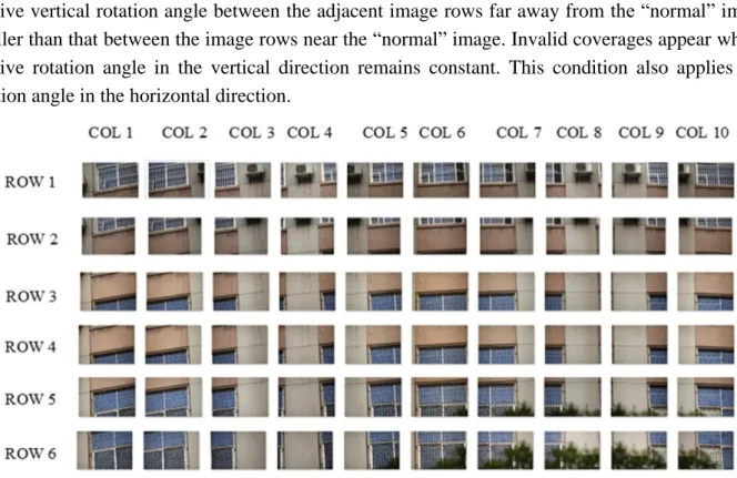
As previously mentioned, the size of a single image sensor is limited, thereby restricting the FOV of DSLRs when long focal lenses are used to yield comparatively high ground resolution images. Therefore, scanning photography was developed. This photography approach obtains sequences of images by rotating the camera in both horizontal and vertical directions to enlarge the FOV of one station. This technique is similar to VisionMap A3 camera, which acquires the flight sequences of frames in a cross-track direction to provide wide angular coverage of the ground [24]. When used in close-range photogrammetry, the presented scanning photography further improves traditional photography by exposing camera frames in both horizontal and vertical directions because the height of the camera is generally difficult to change in a wide range when high targets are photographed. This particular mechanism is similar to the concepts of “cross-track” and “along-track” in aerial photography. Each image captured by the camera is called an original image, and all original images taken at one station form an image matrix as displayed in Figure 1.

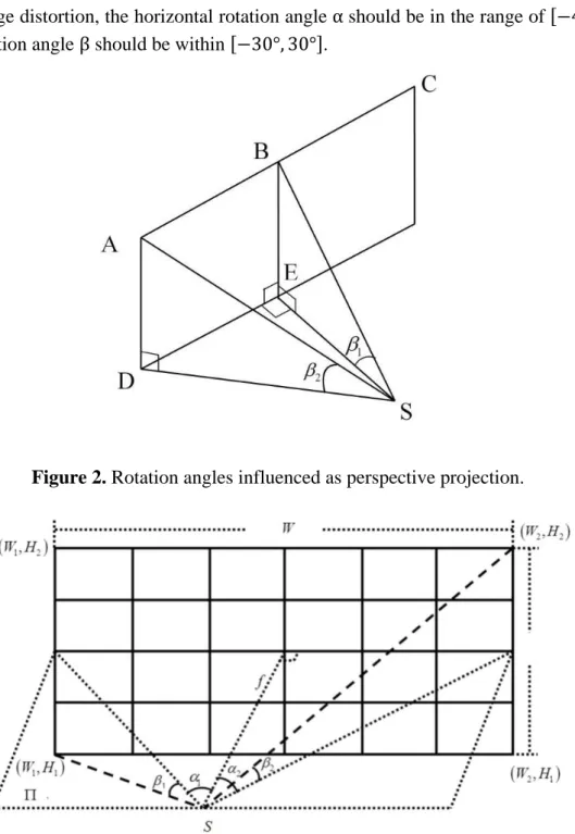
In scanning photography, rotation angles are calculated based on the principle that the relative rotation angles between two adjacent images in both directions are equal. However, in our experiments, this approach is inadequate because the images at the corners of image matrices may be covered by invalid areas as a result of the central perspective when photographing. Figure 2 illustrates how this scenario occurs. In this figure, points D, E, and S are in a horizontal plane, whereas points A, B, C, D and E are in another plane that is perpendicular to the horizontal one. Point B is in line AC, and 𝐴𝐷 ⊥ 𝐷𝐸, 𝐵𝐸 ⊥ 𝐷𝐸, 𝑆𝐸 ⊥ 𝐷𝐸, and 𝑆𝐸 ⊥ 𝐵𝐸. Angles ∠𝐵𝑆𝐸 and ∠𝐴𝑆𝐷 _{are defined as} β₁and β₂, respectively. Therefore, β1 > β2. Points A, B, C, D, and E represent the center points of images A, B, C, D, and E, respectively. Image E is the reference image in both horizontal and vertical directions and is named the “normal” image. β1 denotes the vertical angle rotating from images E to B, and β2 depicts the vertical angle rotating from images D to A. Correspondingly, when photos are taken at the same height, the

relative vertical rotation angle between the adjacent image rows far away from the “normal” image is smaller than that between the image rows near the “normal” image. Invalid coverages appear when the relative rotation angle in the vertical direction remains constant. This condition also applies to the rotation angle in the horizontal direction.

Figure 1. Illustration of image matrix at one station (The matrix contains 6 rows and 10 columns).

In view of the abovementioned problem, we propose an improved means for calculating rotation angles. Figure 3 presents how rotation angles are calculated using this method. S is the perspective center. Horizontal rotation angle ranges from α₁ to α₂, and vertical rotation angle varies from β₁ to β₂. f is the focal length, and region W × H is the ground coverage of the station projected to the focal plane of the “normal” image. The rotation angle of each original image is determined based on the designed overlaps in both directions. In Figure 3, the junctions of grids represent the image centers, and the rays from the perspective center to the image center indicate the principal rays of each image. The mechanism for calculating rotation angles is cited below. By following these procedures, we can calculate the rotation angles of images as in Equation (1).

(1) Obtain the range of rotation angles of a station. As mentioned above, horizontal rotation angle ranges from α₁ to α₂, and vertical rotation angle varies between β₁ and β₂ .

(2) Region W × H can be calculated according to the angle range.

(3) Calculate the temporary horizontal and vertical distances between centers of the adjacent images in the same row and column in image matrix as ∆𝑊_{𝑡𝑒𝑚𝑝} and ∆𝐻_{𝑡𝑒𝑚𝑝}, respectively. Accordingly, determine the row and column number of image matrix as 𝑁_𝑟𝑜𝑤,𝑁_𝑐𝑜𝑙, respectively.

(4) Recalculate the horizontal and vertical distances as ∆𝑊and ∆𝐻, respectively, to divide the region equally into rows 𝑁_𝑟𝑜𝑤 and columns 𝑁_𝑐𝑜𝑙.

(5) Determine the location of each image center on focal plane of the “normal” images, and calculate the rotation angles of each image in both directions.

In our experiment, the absolute value of the horizontal and vertical rotation angles is assumed to be less than 60°. Figure 4 shows the horizontal and vertical rotation angles of original images in one image matrix; where the black solid dots denote the centers of images. In particular, the figure demonstrates that the relative rotation angle between adjacent images is decreased when the rotation angle increases from the “zero position.” The improved results of scanning photography are depicted in Figure 5. To ensure successful measurement, the overlap between any two adjacent images in one image matrix should not be less than 30% in both directions.

To limit image distortion, the horizontal rotation angle α should be in the range of [−45°, 45°], and the vertical rotation angle β should be within [−30°, 30°].

Figure 2. Rotation angles influenced as perspective projection.

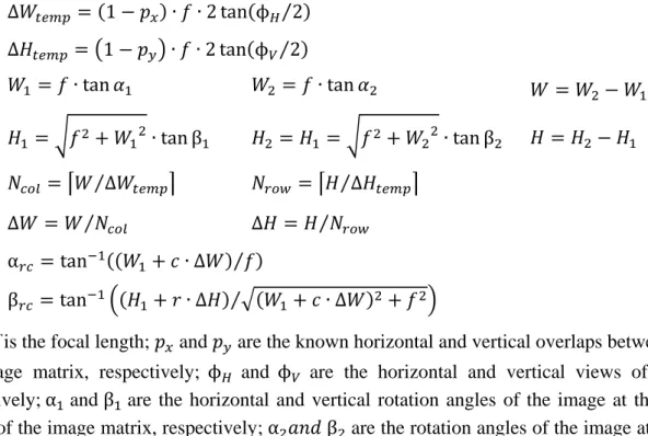
∆𝑊_{𝑡𝑒𝑚𝑝} = (1 − 𝑝_𝑥) ∙ 𝑓 ∙ 2 tan(ϕ_𝐻⁄ ) 2 (1) ∆𝐻_{𝑡𝑒𝑚𝑝}= (1 − 𝑝_𝑦) ∙ 𝑓 ∙ 2 tan(ϕ_𝑉⁄ ) 2 𝑊1 = 𝑓 ∙ tan 𝛼1 𝑊2 = 𝑓 ∙ tan 𝛼2 𝑊 = 𝑊₂− 𝑊₁ 𝐻₁ = √𝑓2_{+ 𝑊} 12∙ tan β1 𝐻2 = 𝐻1 = √𝑓2+ 𝑊22∙ tan β2 𝐻 = 𝐻2 − 𝐻1 𝑁_𝑐𝑜𝑙 = ⌈𝑊 ∆𝑊⁄ _{𝑡𝑒𝑚𝑝}⌉ 𝑁_𝑟𝑜𝑤 = ⌈𝐻 ∆𝐻⁄ _{𝑡𝑒𝑚𝑝}⌉ ∆𝑊 = 𝑊 𝑁⁄ _𝑐𝑜𝑙 ∆𝐻 = 𝐻 𝑁⁄ _𝑟𝑜𝑤 α𝑟𝑐 = tan−1((𝑊1 + 𝑐 ∙ ∆𝑊) 𝑓⁄ ) β_𝑟𝑐 = tan−1_((𝐻 1+ 𝑟 ∙ ∆𝐻) √(𝑊⁄ 1+ 𝑐 ∙ ∆𝑊)2+ 𝑓2)

where f is the focal length; 𝑝_𝑥 and 𝑝_𝑦 are the known horizontal and vertical overlaps between images in the image matrix, respectively; ϕ_𝐻 and ϕ_𝑉 are the horizontal and vertical views of the camera, respectively; α₁ and β₁ are the horizontal and vertical rotation angles of the image at the bottom left corner of the image matrix, respectively; α₂𝑎𝑛𝑑 β₂ are the rotation angles of the image at the top right corner; 𝑊and 𝐻 are the width and height of the projected region on the “normal” image, respectively; ∆𝑊𝑡𝑒𝑚𝑝 denotes the temporary horizontal distance between centers of the adjacent images in the same row in image matrix; ∆𝐻_{𝑡𝑒𝑚𝑝} is the temporary vertical distance between centers of the adjacent images in the same column; 𝑁_𝑟𝑜𝑤 and 𝑁_𝑐𝑜𝑙 are the row and column numbers of the image matrix, respectively; ∆𝑊 represents the distance between adjacent image centers in the same row; ∆𝐻 is the final distance between adjacent image centers in the same column; and α_𝑟𝑐 and β_𝑟𝑐 depict the horizontal and vertical rotation angles of the image at row r and column c in the image matrix, respectively.

Figure 4. Distribution of horizontal and vertical rotation angles; the focal length is 100 mm, and the camera format is 36 mm × 24 mm. The rotation angles of the image at the bottom left corner and top right corner of the image matrix are (−30°, −30°), and (30°, 30°), respectively. The set overlaps in horizontal and vertical directions are 80% and 60%, respectively.

-40 -30 -20 -10 0 10 20 30 40 -40 -30 -20 -10 0 10 20 30 40 vertica l rota tion angle[ °]

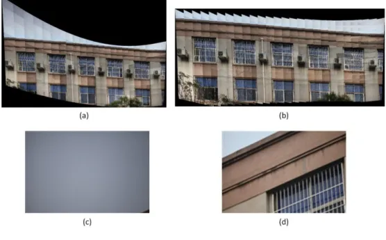
Figure 5. Synthetic images from image matrices with rotation angles calculated in different approaches; (a) is the synthetic image from the image matrix acquired using the same approach in determining the relative rotation angle between adjacent images; (b) is the synthetic image from the image matrix acquired with the improved method introduced in this paper; (c) is the image at the top left corner of the image matrix presented in Figure 5a; (d) is the image at the top left corner of the image matrix presented in Figure 5b.

2.2. Station Distribution

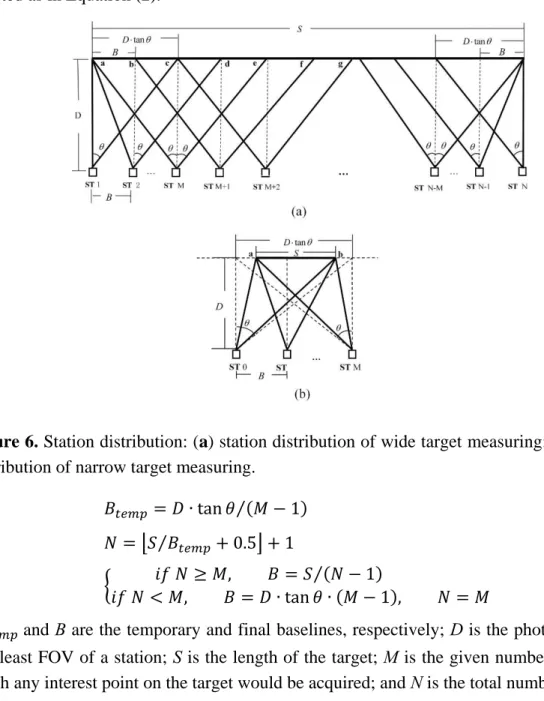
To facilitate data acquisition and processing, our station distribution is set similar to the flight strip in aerial photogrammetry. The top view of this distribution is displayed in Figure 6, where the horizontal line denotes the measured target, the rectangles represent the stations, and the corresponding two solid lines stretching from the station to the object are the FOV of the station. 𝑆 denotes the length of the target, and D is the photographic distance (referred to as photo distance hereafter for brevity). For easy manipulation, the baseline denoted by 𝐵 between adjacent stations is designed the same, which is the same as aerial photogrammetry. Then, the operator will easily find out the location of the next station during data acquisition. To ensure the maximum utilization of images, the columns and rows of each station are varied because the FOV of each station is different. θ is the least FOV of stations determined by operators. 𝑁 represents the total number of stations, and 𝑀 is the given number of least stations from which any interest point on the target would be photographed. Figure 6a shows the station distribution when the target has a large width. In such a case, the distance from the first station to the last is the same as the width of the target. In our scanning photography mechanism, the FOV of stations ranges from 𝜃 to 2θ according to the location of the station. Similarly, the largest intersection angle of the measured points ranges from θ to 2θ. We limit θ between 20° and 45° to maintain a good balance between measurement and matching precisions. Photo distance 𝐷 is determined according to the selected camera focus, required measurement precision, and scene environment. However, certain scenarios exist (e.g., Figure 6b) in which the target is extremely narrow such that the FOV of a station is greatly limited in the given photo distance. Figure 6b depicts the solution for this condition, ensuring the intersection

angle at measuring points. The distance from the first station to the last is larger than the width of the target. As such, the intersection angle at the measuring points is larger than θ, and the view angle of stations can either be smaller or larger than θ. To maintain measurement precision, every point on targets should be photographed from at least three stations. In other words, 𝑀 should be selected, but it should not be less than 3. Then, the overlap between two adjacent stations is set above 67% to enable stereo photogrammetric mapping. It is known that large overlap will result in small baseline. However, as in Figure 6, our scanning photogrammetry is a kind of photogrammetry method using multi-view images. Image correspondences of each tie point for bundle adjustment are from multiple stations, which can form considerable intersection angle. Even if the baseline of the adjacent stations is small, it will not affect the measurement precision. Nevertheless, a small baseline will lead to consuming more time for data obtainment and processing. Therefore, we advise the operators to determine the parameter after balancing the data acquisition time and variation of the target in the depth direction. These parameters are computed as in Equation (2).

Figure 6. Station distribution: (a) station distribution of wide target measuring; (b) station distribution of narrow target measuring.

𝐵_{𝑡𝑒𝑚𝑝}= 𝐷 ∙ tan 𝜃 (𝑀 − 1)⁄

(2) 𝑁 = ⌊𝑆 𝐵⁄ _{𝑡𝑒𝑚𝑝}+ 0.5⌋ + 1

{ 𝑖𝑓 𝑁 ≥ 𝑀, 𝐵 = 𝑆 (𝑁 − 1)⁄ 𝑖𝑓 𝑁 < 𝑀, 𝐵 = 𝐷 ∙ tan 𝜃 ∙ (𝑀 − 1), 𝑁 = 𝑀

where 𝐵_{𝑡𝑒𝑚𝑝} and B are the temporary and final baselines, respectively; D is the photo distance 𝜃; 𝜃 is the given least FOV of a station; S is the length of the target; M is the given number of least stations from which any interest point on the target would be acquired; and N is the total number of stations.

(1) The first station should be aligned to the left edge of the target shown in Figure 6a. However, when faced with the situation as in Figure 6b, the first station should be located at the distance of (𝐷 ∙ 𝑡𝑎𝑛θ − 𝑆)/2, away from the left edge of the target.

(2) The photo distances of every station are approximately equal when the variation of the target in depth direction is not large. Otherwise, the stations should be adjusted to the variation of the target in depth direction to maintain equal photo distances.

(3) The length of the baselines should be the same.

After the location of the first station is identified, the location of the remaining stations can be determined according to the abovementioned principles. As demonstrated in Figure 6a, the horizontal coverage of the first, second, and third stations ranges from points a to c, a to d, and a to e, respectively. Contrarily, the fourth station covers points b to f. The remaining stations follow the same concept. In Figure 6b, points a and b denote the beginning and end of the target, respectively, and the horizontal coverage of each station begins from point a to b.

Since the height of the different parts of the target is variable, the vertical view of each station is based on the height of the photography region. Given that a large pitch angle leads to severe image distortion, the vertical rotation angle of each station should be limited in the range of−30° to 30°. In other words, when the target is extremely high, the height of the instrument or the photo distance must be increased to maintain the vertical view within range.

2.3. Photo Scanner

To guarantee image quality and measurement efficiency, we develop a photo scanner for automatic data acquisition. This scanner shown in Figure 7 consists of a non-metric camera, a rotation platform, a controller (e.g., PC or tablet PC with Win7/8), and a lithium battery. The camera is mounted on the rotation platform composed of a motor unit and transmission mechanism; this platform controls the camera scanning across horizontal and vertical directions. Figure 7 indicates that the rotation center of the platform is not the perspective center of the camera. However, when the scanner is used for large engineering measurements, the offset values are relatively tiny compared with photo distance. A module for determining rotation angles is also integrated into the software to transmit data and control platform rotation. The scanner automatically obtains the image once the camera parameters (i.e., focus and image format), data storage path, horizontal and vertical overlaps between images in each image matrix, and ground coverage of stations are inputted into the software by the operators. For convenient measurement, the scanner is designed to be mounted on a tripod for the total station, and the battery unit for the rotation platform can be hung on the tripod. Thus, the developed photo scanner can be carried and operated by only one person when conducting measurements, providing great convenience.

The mechanism for applying the developed scanner is as follows: (1) The instrument is installed and placed at the proper position.

(2) The photographic plane is paralleled to the average plane of the needed photographing region, and the rotation platform is leveled with the bubble on the instrument base. This position of the camera is defined as the “zero posture” in this station and is considered the origin of rotation angles in both horizontal and vertical directions.

(3) The FOV of this station is specified, and the required parameters are inputted into the controller. (4) The number of rows and columns of the image matrix as well as the rotation angles in horizontal and vertical directions for each image are computed, and the signal is sent to manage the rotation and exposure of the camera for automatic image acquisition.

Data can be stored by transferring images into the controller (e.g., PC or tablet PC) and storing them in a compact flash card. In the second method, the images from the camera are not required to be transmitted to the PC or tablet PC. As such, the photo interval is shorter. During photographing, the controller enables a real-time quick view of the captured images. At the same time, the rotation angles of each captured image are stored in the controller as a log file, which can be used as auxiliary information for data processing.

Figure 7. Parts of the photo scanner

2.4. Data Processing

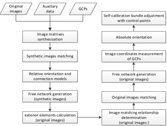
In our proposed method, data are automatically processed once the user specifies the data directory and required outputs. To achieve high accuracy and stable solution, all original images are used for bundle adjustment because redundant observations are helpful in obtaining a robust solution, and information loss is unavoidable during image synthesis. Considering that all original images are needed for bundle adjustment, we employ modified triangulation to improve the efficiency of data organization and processing. As previously noted, the core idea of modified triangulation is that although the overlaps between original images from different stations remain unknown, we can estimate the overlaps between coverages of image matrices according to the station distribution. Thus, we use the images synthesized from the image matrix to generate a free network. We then compute the initial exterior elements of original images in this free network from the elements of synthetic images and rotation angles of original images. After the matching relationships among the original images from neighboring image matrices are identified according to the matching results of the two corresponding synthetic images, image matching is executed among original images to determine tie points. Self-calibration bundle adjustment with control points is then performed. In establishing the initial exterior parameters of original images,

we assume that the perspective centers of original images and their corresponding synthetic images are the same even though they are actually different. The accurate exterior parameters of original images that vary from those of the corresponding synthetic images can be obtained after bundle adjustment. Figure 8 exhibits the flow of data processing. The processes of taking original images with long focal lens into bundle adjustment are determined to be similar to that using the VisionMap A3 system. Thus, this procedure is valid and can be used in both aerial and close-range photogrammetry.

Figure 8. Flow chart of data processing 2.4.1. Synthetic Image

In practical measurements in scanning photography, the unknown overlaps between stereo pairs of original images from different stations are not always large enough for relative orientation. This condition therefore leads to an unstable relative orientation among stereo pairs. Considering that the overlaps between station image matrices are large enough for relative orientation, we apply a simplified method of synthesizing image matrices for free network generation. In view of information loss when original images are synthesized from image matrices, synthetic images are not used for final bundle adjustment but are only used for computing the initial exterior elements of original images. Although the camera is not rotated around the perspective center, the offset values from its center to the center of rotation are relatively tiny compared with the photo distance when performing large engineering measurements using the developed photo scanner. Therefore, we simplify the model by ignoring the offset values and projecting the image matrix to the focal plane of the “normal” image to synthesize the image matrix. Figure 9 illustrates the image synthesis model. For simplicity, only one row of the image matrix is graphed. The rotation angles of the images can be presented as (𝐻_𝑖, 𝑉_𝑖) (𝑖 = 1,2, … , 𝑚) . 𝐻_𝑖 and 𝑉_𝑖 are the horizontal and vertical angles, respectively, and m is the number of images in the image

Image matrixes synthesization

Synthetic images matching

Free network generation (synthetic images)

exterior elements calculation (original images)

Image matching relationship determination (original images ) Original images matching Image coordinates measurement

of GCPs Absolute orientation Self-calibration bundle adjustment

with control points

Free network generation (original images) Relative orientation and

connection models Original

images

Auxiliary

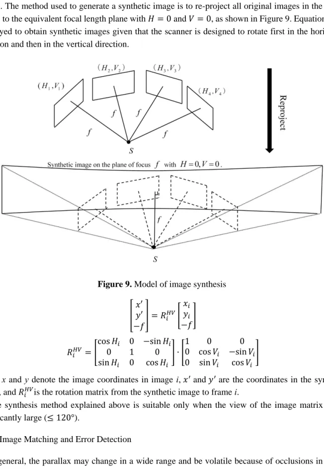
matrix. The method used to generate a synthetic image is to re-project all original images in the image matrix to the equivalent focal length plane with 𝐻 = 0 and 𝑉 = 0, as shown in Figure 9. Equation (3) is employed to obtain synthetic images given that the scanner is designed to rotate first in the horizontal direction and then in the vertical direction.

Figure 9. Model of image synthesis

[ 𝑥′ 𝑦′ −𝑓] = 𝑅𝑖 𝐻𝑉_[ 𝑥_𝑖 𝑦_𝑖 −𝑓] (3) 𝑅_𝑖𝐻𝑉 = [ cos 𝐻_𝑖 0 −sin 𝐻_𝑖 0 1 0 sin 𝐻_𝑖 0 cos 𝐻_𝑖 ] ∙ [ 1 0 0 0 cos 𝑉_𝑖 −sin 𝑉_𝑖 0 sin 𝑉_𝑖 cos 𝑉_𝑖 ]

where x and y denote the image coordinates in image i, 𝑥′ and 𝑦′ are the coordinates in the synthetic image, and 𝑅_𝑖𝐻𝑉_{is the rotation matrix from the synthetic image to frame i.}

The synthesis method explained above is suitable only when the view of the image matrix is not significantly large (≤ 120°).

2.4.2. Image Matching and Error Detection

In general, the parallax may change in a wide range and be volatile because of occlusions in close-range image pairs. When the relative rotation angle is larger than 15°, which commonly occurs in oblique photography, traditional image matching is unsuitable. Alternatively, scale-invariant feature transform (SIFT) match can be steadily applied in many cases when it involves an angle that is less than 50° [38]. Given that the SIFT features presented by 128-dimensional vectors are used for image matching, a long computational time is needed when a large number of feature points are involved. Thus, graphics

processing unit (GPU) acceleration is employed. Considering that the memory of GPUs is limited, we perform a block-matching algorithm. In this algorithm, we simply use each block from one image to match all of the blocks from another image. The block matching results are accepted only when the number of correspondences is larger than the threshold.

Mismatching inevitably occurs in image matching methods. Thus, we should pay attention to error detection. The outliers in SIFT point matches are generally discarded with random sample consensus (RANSAC) for estimating model parameters. In our scanning photography, two kinds of error detection can be used after image matching, and the method to be applied is selected based on whether the corresponding points are from the same station. For matching images from the same station, the object coordinates of perspective centers are approximately equal. Therefore, the homography model [39] in Equation (4) is used as the estimation model. The geometric distortions between images are severe when the matching images are acquired from different stations, suggesting that transformation models (e.g., affine and projective transforms) are no longer suitable for detecting matching errors [40]. After performing several experiments, we adopt the quadric polynomial model in Equation (5) to estimate geometric distortions. This model is the superior choice in terms of computational time and measurement precision. The threshold of residual for RANSAC should be relaxed because the interior elements of original images are inaccurate, and the estimation model is not rigid.

[𝑦′𝑥′ 1 ] [ ℎ₁ ℎ₂ ℎ₃ ℎ₄ ℎ₅ ℎ₆ ℎ7 ℎ8 ℎ9 ] ∙ [ 𝑥 𝑦 1] (4)

where(𝑥, 𝑦) and (𝑥′, 𝑦′) are the image coordinates on the left and right images in an image pair, respectively, ℎ₁ ,ℎ₂, …,ℎ₉ are elements of the homography matrix, and ℎ₉ = 1.

𝑥′_{= 𝑎}

1𝑥2+ 𝑎2𝑥𝑦 + 𝑎3𝑦2+ 𝑎4𝑥 + 𝑎5𝑦 + 𝑎6

(5) 𝑦′_{= 𝑏}

1𝑥2+ 𝑏2𝑥𝑦 + 𝑏3𝑦2+ 𝑏4𝑥 + 𝑏5𝑦 + 𝑏6 where 𝑎1,𝑎2,…, 𝑎6, and 𝑏1, 𝑏2, …, 𝑏6 are quadric polynomial coefficients. 2.4.3. Modified Aerial Triangulation

The overlaps between synthetic images are known based on station distribution. Therefore, these images, instead of the original ones, are more suitable for interpreting epipolar geometry. The reason is that the overlaps among original images are unknown before the pre-processing of image matching. Thus, we use synthetic images in the triangulation of relative orientation and model connection to generate a free network. In close-range photogrammetry, the initial elements of relative orientation are crucial to achieving good solution in triangulation when intersection angles are large. In this event, a stable algorithm of relative orientation is required. Compared with other direct methods (e.g., 6-, 7-, and 8-point methods), the 5-point method performs best in most cases [41]. For this reason, we apply the 5-point relative orientation algorithm proposed by Stewenius [42] from the perspective of algebraic geometry. This algorithm employs a Gröbner basis to easily explain the solution [42]. To improve precision, an iterative scheme for refining relative orientation is adopted after the calculation of initial parameters. Each successive model is then connected with one another similar to the case in aerial triangulation. Correspondingly, the free network of synthetic images is established.

The free network provides the exterior orientation elements of synthetic images. However, the exterior orientation elements of each original image are the required parameters for final bundle adjustment. Given that the changes are small among the space coordinates of each original image perspective center in one image matrix, the initial space coordinates of the original image are considered similar to those of their corresponding synthetic image. Accordingly, we can solve the azimuth elements of original images by decomposing the rotation matrix calculated with the azimuth elements of synthetic images and rotation angles of original images as depicted in Equation (6).

𝑅𝑗𝑖 = 𝑅𝑗∙ 𝑅𝑗𝑖𝐻𝑉 (6)

where 𝑅_𝑗𝑖 is the rotation matrix of image i in station j , 𝑅_𝑗 is the rotation matrix of synthetic image j in the free network, and 𝑅_𝑗𝑖𝐻𝑉 _{is the rotation matrix of relative rotation angles from the synthetic image of} station j to image i.

Before bundle adjustment with all original images, image matching should be executed among original images to obtain the corresponding points as tie points for bundle adjustment. Stereo matching is performed between the original images from different stations as well as between the original images from the same station. We find six images, namely, two from the same station and four from the next station, which overlap with each original image to proceed with matching. For the images from the same station, we chose the two images at the right of and below the processing image in the image matrix. Meanwhile, for the images from the next station, we chose four images with the highest overlapping rate with the image for stereo matching. The overlapping rate is calculated according to the matching results of the two corresponding synthetic images. Then, we tie all matching results together and then use multi-image forward intersection to compute the space coordinates of the tie points in the free network. As a result, the free network of original images is established. Absolute orientation is performed to establish the relationship between the space coordinate system of free network and the object space coordinate system before bundle block adjustment. We then compute the exterior elements of original images and space coordinates of tie points in the object space coordinate system.

In general, traditional bundle adjustment is the most mature approach because the collinearity condition for all tie points (TPs) and ground control points (GCPs) are satisfied simultaneously [43]. Considering the instability of intrinsic parameters of non-metric cameras, we utilize the on-line self-calibration bundle adjustment with control points to obtain the final result. In consideration of the camera intrinsic parameters, radial distortion, and tangential distortion, the mathematical model of self-calibration bundle adjustment based on the collinearity equation is established as in Equation (7) [44].

𝑥 − 𝑥₀− ∆𝑥 = −𝑓𝑎1(𝑋 − 𝑋𝑆𝑖) + 𝑏1(𝑌 − 𝑌𝑆𝑖) + 𝑐1(𝑍 − 𝑍𝑆𝑖) 𝑎₃(𝑋 − 𝑋_𝑆𝑖) + 𝑏₃(𝑌 − 𝑌_𝑆𝑖) + 𝑐₃(𝑍 − 𝑍_𝑆𝑖) (7) 𝑦 − 𝑦0− ∆𝑦 = −𝑓 𝑎₂(𝑋 − 𝑋_𝑆𝑖) + 𝑏₂(𝑌 − 𝑌_𝑆𝑖) + 𝑐₂(𝑍 − 𝑍_𝑆𝑖) 𝑎₃(𝑋 − 𝑋_𝑆𝑖) + 𝑏₃(𝑌 − 𝑌_𝑆𝑖) + 𝑐₃(𝑍 − 𝑍_𝑆𝑖) where ∆𝑥 = (𝑥 − 𝑥₀)(𝑘₁𝑟2_{+ 𝑘} 2𝑟4) + 𝑝1[𝑟2+ 2(𝑥 − 𝑥0)2] + 2𝑝2(𝑥 − 𝑥0)(𝑦 − 𝑦0) (8) ∆𝑦 = (𝑦 − 𝑦0)(𝑘1𝑟2+ 𝑘2𝑟4) + 𝑝2[𝑟2+ 2(𝑦 − 𝑦0)2] + 2𝑝1(𝑥 − 𝑥0)(𝑦 − 𝑦0) 𝑟2 _{= (𝑥 − 𝑥} 0)2 + (𝑦 − 𝑦0)2

where (x, y) is the image coordinate of a point in image i; [𝑋, 𝑌, 𝑍]is the object coordinate of the point; [𝑋_𝑆𝑖, 𝑌_𝑆𝑖, 𝑌_𝑆𝑖] is the object coordinate of perspective center of image i; 𝑎₁,𝑎₂, 𝑎₃, 𝑏₁, 𝑏₂, 𝑏₃, 𝑐₁, 𝑐₂, and 𝑐₃ are elements of the rotation matrix of image i; f is the focal length; (𝑥₀, 𝑦₀) denotes the coordinate of the principal point of image i; (∆𝑥, ∆𝑦) denotes the correction of the lens distortion; 𝑘₁ and 𝑘₂ are radial distortion coefficients; and 𝑝₁ and 𝑝₂ are tangential distortion coefficients.

During bundle adjustment, we can establish several correspondence pairs for each tie point, and the corresponding points can be either from the same station or from different stations. The pairs from the different stations are characterized by large intersection angles that are beneficial to the accuracy of depth direction, whereas the pairs from the same station are characterized by very small intersection angles that may lower accuracy. Thus, we consider the observations of image coordinates of tie points as correlative rather than independent, and the correlation coefficient is inversely proportional to the intersection angle. The weight of observations is based on intersection angles as considered in bundle adjustment and the weight of the ground points is set to 10 times the tie points. Iterative least squares adjustment is exploited for solving the unknown parameters of original images. Finally, accurate solutions are yielded for all images.

3. Experimental Results 3.1. Experimental Data

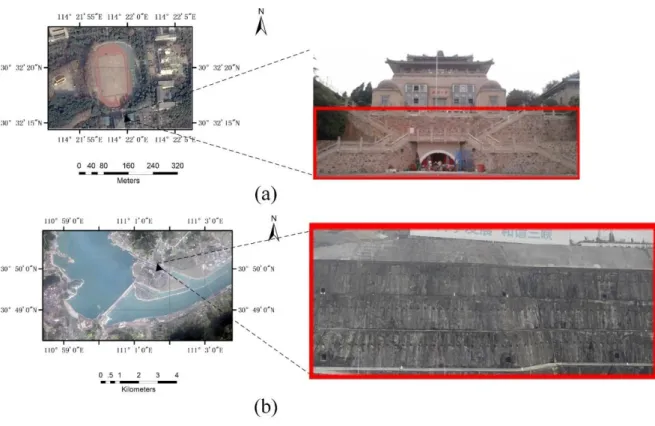
Scanning photogrammetry has been proposed mainly for acquiring data when large targets are measured and for obtaining accurate measurements of large objects at any focal length. Here, we emphasize in our experiments the application of cameras with long focal lens. Our method has been proven effective in experiments involving measuring the flag platform of Wuhan University and the high slope of Three Gorges Project permanent lock, as shown in Figure 10. The Cannon 5D Mark II camera (format size: 5616 × 3744, pixel size: 6.4 μm) is used for the tests. In the experiments, reflectors for the total station are used as control points. Object surfaces will cause reflectors to be attached unevenly because the surfaces may be rough. We use plexiglass boards, which are thicker, as the baseplates of reflectors to ensure that the reflectors attached to the object surfaces are even. Figure 10a shows a quick view of the flag platform. The height, width, and depth of this area are 10, 35, and 12 m. As shown in the figure, there are stairways leading to the flag platform from the playground, resulting in several layers in the measurement area, which brings difficulty in data processing because of the discrete relief displacement. Control points are measured by Sokkia SET1130R3 total station with 3 mm accuracy. Figure 10b shows a quick view of the high slope of Three Gorges Project permanent lock. The height, width, and depth of this region is 70, 150, and 70 m. Owing to the special environment in this field, the best position for measurement is the opposite side of the lock. The photo distance can reach up to 250 m. The Leica TCRA1201 R300 total station is used to measure control points with an accuracy of 2.9 mm.

Figure 10. Quick view of test fields. ((a) flag platform of Wuhan University.; (b) high slope of Three Gorges Project permanent lock. The regions in the red rectangles show the measuring ranges.)

3.2. Results of Synthetic Images

Figure 11 illustrates the synthetic images of the two test fields. Figure 11a shows the synthetic image of one station for the field test of the flag platform with 300 mm focus lens, and the photo distance is 40 m. Figure 11b shows the synthetic image of one station for test field of the high slope of Three Gorges Project permanent lock with 300 mm focus lens at a distance of 250 m. The method applied to yield synthetic images is described in Section 2.4.1. As shown, the invalid area in the synthetic images is slightly due to the use of the improved method. The performance is not that good, because no post-processes, such as unifying color or finding best seam lines, are executed. However, these factors do not have much influence on the matching of synthetic images.

3.3. Results of Image Matching (Synthetic Images and Original Images)

Three kinds of image matching exist in this process: one for synthetic images, one for original images from different stations, and one for original images from the same station. For synthetic images, every two overlapping images is a stereo pair. However, for original images, only two overlapping images from different stations can form a stereo pair. Both stereo pairs and non-stereo pairs are needed to be matched with the SIFT matching method. After SIFT matching is performed, error detection methods are used to refine the matching results. Depending on whether the image pair is a stereo pair or a non-stereo pair, RANSAC with estimation by quadric polynomial or homography model is used for detecting errors.

Figures 12 and 13 show the results of matching and mismatching points in synthetic images from two stations. The red crosses denote the detected correct corresponding points, whereas the blue crosses denote the detected errors. The detection model is a quadric polynomial model. The matching results of the original images are shown in Figures 14–17. Image pairs in Figures 14 and 16 are stereo pairs and are processed by quadric polynomial models. Meanwhile, image pairs in Figures 15 and 17 are non-stereo pairs and are processed by homography models. The results verify that these error detection methods are valid. Given that an amount of feature points are extracted from the images showed in Figures 14 and 15, we perform block-matching algorithm. Thus, matching errors clustering exists because of the mechanism of our block-matching algorithm. However, our error detection method can eliminate outliers efficiently.

Figure 11. Synthetic images: (a) synthetic image of one station for test field showed in Figure 10a; (b) synthetic image of one station for test field showed in Figure 10b.

Figure 12. Synthetic images matching. (a,b) shows the matching results of synthetic images from the first and second station for test field in Figure 10a; (c,d) illustrates part of the results.

Figure 13. Synthetic images matching. (a,b) shows the matching results of synthetic images from the first and second station for test field in Figure 10b; (c,d) illustrates part of the results.

Figure 14. Original images matching. (a,b) shows the matching results of images from the adjacent stations as measuring the first field showed in Figure 10a; (c,d) illustrates part of the results.

Figure 15. Original images matching. (a,b) shows the matching results of adjacent images in the same row of one image matrix as measuring the first field showed in Figure 10a; (c,d) illustrates part of the results.

Figure 16. Results of stereo images matching. (a,b) shows the matching results of images from the adjacent stations as measuring the second field showed in Figure 10b; (c,d) illustrates part of the results.

Figure 17. Results of stereo images matching. (a,b) shows the matching results of adjacent images in the same row of one image matrix as measuring the second field showed in Figure 10b; (c,d) illustrates part of the results.

3.4. Results of Point Clouds

The free network of original images is generated after the correspondences of original images are tied together. The generated point cloud is a mess, because exterior parameters of images are not computed accurately and interior parameters of the camera have not been calibrated at the moment. After self-calibration bundle adjustment with control points, the point cloud will become regular and present the sketchy model of the target. Figures 18 and 19 show the difference of the point cloud of two test fields before and after self-calibration bundle adjustment with control points.

3.5. Coordinate Residuals of Triangulation

We conduct several groups of comparative experiments to evaluate the effects of different factors, such as photo distance, overlapping rate between original images in image matrices, given number of least stations (𝑀)from which any interest point on the target are acquired, set intersection angle(𝜃), and focal length, on the measurement accuracy in scanning photogrammetry. In the first test field of the flag platform, we analyze the effects of the four factors by using a camera with a 300 mm lens. In the second test field, the high slope at permanent lock of Three Gorges Project, two lenses with 300 and 600 mm lenses are used in evaluating the effects of focal length.

Figure 18. Point clouds. (a,b) shows the point clouds before and after self-calibration bundle adjustment with control points in the experiment of the first field showed in Figure 10a.

Figure 19. Point clouds. (a,b) shows the point clouds before and after bundle adjustment in the experiment of the second field showed in Figure 10b.

3.5.1. Comparison of Different Photo Distances

To evaluate the measurement accuracy from different photo distances when using scanning photogrammetry, the images of the first test field are obtained from 40, 80, and 150 m, and the ground resolutions are 0.9, 1.7, and 3.2 mm, respectively. Experiments are correspondingly named as cases I, II, and III. The horizontal and vertical overlaps between original images in image matrices in the three cases are set the same, 80% and 60%, respectively. We adjust the baseline of the stations to ensure that the station numbers of the three experiments are equal; that is, the intersection angles of the three experiments are different.

Table 1 displays the details of this experiment, and Figure 20 shows the error vectors. To compare the influence of photo distances in scanning photogrammetry, we choose 12 points as control points from 26 points distributed evenly in the test area, and the rest are check points. Owing to the angle existing between the average plane of the measured target and the XY plane in the chosen object coordinates, the distribution of control and check points on the right side of the picture is denser than that on the left side of pictures. Moreover, as shown in Table 1, the mean intersection angle of tie points is smaller than the set least intersection angle. The reason is that many of the tie points only appear in two adjacent stations.

Table 1. Parameters and coordinate residuals of experiments for first test field at different photo distances.

Cases I II II III III

Photo distance (m) 40 80 80 150 150

Focal length (mm) 300

Ground resolution (mm) 0.9 1.7 1.7 3.2 3.2

Total station number N 5

Give least intersection angle θ (°) 26 35 35 35 35

Baseline (m) 8.8 14 14 26.3 26.3

Image amount 858 171 171 41 41

RMSE of image point residuals (pixel) 1/2 1/2 1/2 1/2 1/2 Mean intersection angle of tie points (°) 23.7 18.5 18.5 18.1 18.1 Maximum intersection angle of tie points (°) 43.2 37.6 36.4 35.8 35.6 Minimum intersection angle of tie points (°) 4.2 4.4 4.8 6.3 6.5

Number of control points 12 12 10 12 8

Accuracy (mm) X 1.2 1.8 1.6 1.5 1.5 Y 1.0 1.3 0.7 1.2 0.4 Z 1.1 2.2 2.7 2.5 2.9 XY 1.5 2.2 1.7 1.9 1.5 XYZ 1.9 3.1 3.2 3.1 3.3

Number of check points 14 14 16 14 18

Accuracy (mm) X 2.0 2.1 2.4 2.5 2.5 Y 0.8 1.8 1.9 1.6 1.7 Z 1.0 2.5 2.5 2.8 2.7 XY 2.1 2.8 3.0 2.9 3.0 XYZ 2.3 3.7 3.9 4.0 4.1

Figure 20. Error vectors of control points and check points. (a) is the error vectors of points measured at a distance of 40 m; (b) and (c) denote error vectors of points measured at a photo distance of 80 m. (b) is the result with 12 control points, and (c) is 10 control points; (d) and (e) show error vectors at a photo distance of 150 m, and they are the results with 12 control points and eight control points, respectively.

As shown by the results in Table 1, scanning photogrammetry can achieve high accuracy even when measurement is performed from different photo distances. If ground sampling distance increases (which occurs if the photo distance also increases), then the pixel becomes larger when projected on the object, and less detail can be captured. As ground sampling distance increases, fine details become visible, which improves measurement accuracy. In this experiment, the accuracy of the control points measured by total station and the ground sampling distance are in the same magnitude, and the accuracy of the control points measured by total station is even larger than that of the ground sampling distance, thus causing the measurement accuracy to not be proportional to the photo distance. At the same time, the accuracy measured by the total station in the X-direction is the lowest. Therefore, in case I, the final

measurement accuracy in the X-direction is lower than that in other directions because of its dependence on the accuracy measured by the total station. To further analyze the necessary amount of control points, we decrease the number of control points to 10 and 8 in cases II and III, respectively. The measurement results in Table 1 reveal that necessary control points decrease when the photo distance increases, which is related to the relief displacement of the target on images.

3.5.2. Comparison of Different Overlaps between Images in Image Matrices

In data acquisition, the number of original images that should be taken at one station is determined by the overlaps between images in image matrices. However, more images will relate to additional time spent on data acquisition and processing. Therefore, we prefer to minimize overlaps without affecting measurement accuracy. To analyze the influence of the horizontal overlapping rate in the image matrix on measurement accuracy, data with different horizontal overlaps (80%, 60%, and 30%) are obtained in the flag platform at a photo distance of 40 m. The detailed parameters and coordinate residuals of control and check points are shown in Table 2. Figure 21 displays the error vectors. The experiment results reveal that horizontal overlaps in the image matrix affect measurement accuracy; that is, accuracy is lowered with the reduction of horizontal overlap. However, the influence is insignificant. We can deduce that the vertical overlap follows a similar way. Therefore, we can conclude that when the required precision is met, the horizontal and vertical overlaps can be decreased to improve the efficiency of data acquisition and processing. Meanwhile, experience dictates that the overlapping rate cannot be less than 30% in both directions to guarantee successive data processing.

Figure 21. Error vectors of control points and check points. (a), (b), and (c) denote error vectors of points with horizontal overlap of 80%, 60%, and 30%, respectively. The coordinate residuals of check points in the experiments with image horizontal overlap 80%, 60%, and 30%, respectively.

Table 2. Parameters and coordinate residuals of experiments for first test field at different horizontal overlaps of image matrix.

Cases I II III

Photo distance (m) 40 40 40

overlap in horizontal direction 80% 60% 30% overlap in vertical direction 60% 60% 60%

Focal length (mm) 300

Ground resolution (mm) 0.9

Total station number N 5

Give least intersection angle θ (°) 26

Baseline (m) 8.8

Image amount 858 444 232

RMSE of image point residuals (pixel) 1/2 1/2 1/2 Mean intersection angle of tie points (°) 23.7 23.4 22.5 Maximum intersection angle of tie points (°) 43.2 43.2 43.0 Minimum intersection angle of tie points (°) 4.2 5.6 2.4

Number of control points 12 12 12

Accuracy (mm) X 1.2 1.5 1.6 Y 1.0 1.1 1.2 Z 1.1 1.5 1.6 XY 1.5 1.9 2.0 XYZ 1.9 2.4 2.6

Number of check points 14 14 14

Accuracy (mm) X 2.0 2.0 1.9 Y 0.8 0.7 0.7 Z 1.0 1.4 1.8 XY 2.1 2.1 2.1 XYZ 2.3 2.5 2.7 3.5.3. Comparison of M

According to the station distribution in our scanning photogrammetry, the baseline between stations decreases as the value of the given number of least stations from which any interest point on the target would be photographed (M) increases. A shorter baseline is known to be conducive to image matching; however, the number of images in the project will be increased, which would require more time for data acquisition and processing. To analyze the influence of M, we conduct two experiments that measure the flag platform from three and five stations each at a photo distance of 80 m. The parameters and coordinate residuals of control points and check points are listed in Table 3. Figure 22 shows the error vectors of these points. In this experiment, the relief is small from this photo distance, suggesting that M rarely influences measurement accuracy. However, if the relief is large, M should be increased. We recommend that the value of 𝑀should be no less than 3.

Table 3. Parameters and coordinate residuals of experiments for first test field at different values of M.

Cases I II

Photo distance (m) 80 80

overlap in horizontal direction 80% 80% overlap in vertical direction 60% 60%

Focal length (mm) 300

Ground resolution (mm) 1.7

Total station number N 3 5

Give least intersection angleθ (°) 35 35

Baseline(m) 28 14

Image amount 90 171

RMSE of image point residuals(pixel) 1/2 1/2 Mean intersection angle of tie points(°) 25.2 18.5 Maximum intersection angle of tie points(°) 36.3 36.4 Minimum intersection angle of tie points(°) 3.4 4.8

Number of control points 10 10

Accuracy (mm) X 1.6 1.6 Y 0.8 0.7 Z 2.6 2.7 XY 1.8 1.7 XYZ 3.2 3.2

Number of check points 16 16

Accuracy (mm) X 2.4 2.4 Y 1.7 1.9 Z 2.5 2.5 XY 3.0 3.0 XYZ 3.9 3.9

Figure 22. Error vectors of control points and check points. (a) and (b) denote error vectors of points in the experiments of obtaining images from three and five stations Coordinates residuals of check points in the experiments with M as 3 and 5, respectively.

3.5.4. Comparison of Set Intersection Angle

In this part, experiments with different intersection angles are conducted. The intersection angle is set to 26° and 35° in the two tests at a photo distance of 40 m. According to the abovementioned rules of station distribution, the amounts of total stations are 3 and 5, respectively. Table 4 lists the detailed parameters of the experiments and the coordinate residuals. Figure 23 shows the error vectors. The results unexpectedly demonstrate that a larger intersection angle corresponds to a lower measurement accuracy. We speculate that the main cause of this situation is increase in the photo distortion when the intersection angle is enlarged. Therefore, a large intersection angle is not always better than a smaller intersection angle and should be determined according to the relief displacement of the measuring target.

Table 4. Parameters and coordinate residuals of experiments for first test field at different intersection angles.

Cases I II

Photo distance (m) 40 40

overlap in horizontal direction 80% 80%

overlap in vertical direction 60% 60%

Focal length (mm) 300

Ground resolution (mm) 0.9

Total station number N 5 3

Give least intersection angleθ (°) 26 35

Baseline (m) 8.8 17.6

Image amount 858 738

RMSE of image point residuals (pixel) 1/2 1/2 Mean intersection angle of tie points (°) 23.7 29.9 Maximum intersection angle of tie points (°) 43.2 44.8 Minimum intersection angle of tie points (°) 4.2 6.1

Number of control points 12 12

Accuracy (mm) X 1.1 1.3 Y 1.0 1.1 Z 1.2 1.4 XY 1.4 1.7 XYZ 1.9 2.2

Number of check points 14 16

Accuracy (mm) X 2.0 1.8 Y 0.8 0.8 Z 1.0 1.9 XY 2.1 2.0 XYZ 2.3 2.7

Figure 23. Error vectors of control points and check points. (a) and (b) demonstrate error vectors of points in the experiments with designed intersection angle as 26°and 35°.

3.5.5. Comparison of Different Focuses

Ground sampling distance can be improved by increasing the focal length of the camera, which can be beneficial to measurement accuracy. In this part, two lenses with focus lenses of 300 mm and 600 mm are used for measuring the high slope in the second field (Figure 10b). The tests are named Cases I and II, respectively. Table 5 shows the detailed parameters of the experiments and the coordinate residuals, and Figure 24 illustrates the error vectors. The scene of the field is complex and thus can only be surveyed at a long distance of 250 m. A total of 14 control points are selected for orientation. Table 5 shows that our scanning photogrammetry can achieve high precision when a large target from a long distance is measured. This efficient measurement in Case II reveals that our method is valid and can apply telephoto lens to achieve high precision with a few control points. However, the residuals in case II is expected to improve much more than that in case I because the ground sampling distance in case II is improved to half of that in case I. However, the accuracy was not improved substantially because the accuracy was limited by the accuracy of the control points measured by the total station. Another reason is the systematic errors that cannot been corrected completely because the distortion in images obtained with telephoto lenses is complicated. Therefore, finding ways to solve this problem is the main concern of our future works.

Figure 24. Error vectors of control points and check points. (a) and (b) demonstrate error vectors of points in the experiments with 300 and 600 mm focal lens.

Table 5. Parameters and coordinate residuals of experiments for second test field at different focuses.

Cases I II

Photo distance (m) 250 250

overlap in horizontal direction 80% 60% overlap in vertical direction 60% 40%

Focal length (mm) 300 600

Ground resolution (mm) 5.3 2.7

Total station number N 3 3

Give least intersection angleθ (°) 30 30

Baselines (m) 55 55

Image amount 601 982

RMS of image point residuals (pixel) 2/5 1/2 Mean intersection angle of tie points(°) 22.2 23.4 Maximum intersection angle of tie points(°) 33.1 29.4 Minimum intersection angle of tie points(°) 6.1 6.0

Number of control points 14 14

Accuracy (mm) X 3.3 1.7 Y 3.3 1.6 Z 3.9 4.4 XY 4.6 2.3 XYZ 6.0 5.0

Number of check points 14 14

Accuracy (mm) X 3.2 2.7 Y 4.0 3.2 Z 4.4 3.9 XY 5.1 4.2 XYZ 6.8 5.7 4. Discussion

This paper uses scanning photography to solve the problem of data acquisition and organization caused by the limited FOV of digital cameras when measuring large targets with long focal lens. When cameras with long focal lens are used to measure large targets, the ground coverage is small, resulting in the need to take lots of images. If all these images are taken manually, then only experienced photographers can accomplish the work well. Otherwise, coverage gaps will occur, especially when applying multi-view photography to obtain images to maintain measurement precision. Scanning photography combined with the isometric station distribution proposed in this paper is designed to obtain images regularly, as in data acquisition in aerial photogrammetry. Also, it is a kind of photogrammetry method using multi-view images. After operators input the required parameters, the photo scanner automatically obtains images, thus making it easy to acquire images without coverage gap and to organize images for data processing. Moreover, the photo scanner can record the rotation angle of each image when obtaining images, which can be used in data processing as auxiliary information. A modified triangulation is conducted according to the traits of the data acquired by scanning photography that the

overlaps among images from the same station are known, improving the efficiency and stability of data processing. The modified triangulation can be considered as a kind of global structure from motion (SFM) with auxiliary information.

Successfully used in aerial and close-range photogrammetry, scanning photography is the approach of controlling the camera to rotate around one point to acquire images to enlarge the field-view-of one station. Vision Map A3 system is an example of scanning photography in aerial photogrammetry. The camera used in this system consists of dual CCD detectors with two 300 mm lenses. As the flight moves when obtaining images, the camera can only be controlled to rotate in a cross-track direction, which provides a field-of-view of 104°. In the along-track direction, the field-of-view is enlarged by using dual CCDs. Traditional triangulation with GPS information is utilized for data processing. After that, super large frames synthesized from all pairs of original images of one sweep are generated for stereo photogrammetric mapping [24]. In close-range, the platform for obtaining images is static and always controls only one camera rotating in both horizontal and vertical directions (the same as along-crack and cross-crack direction) to enlarge the field of view. While, several systems take images both with normal and long focal lenses in measurements; normal focal lens images are used to provide a general network around the object, whereas the long focal lens images are employed to ensure accuracy and reconstruct the ‘sharp’ details [30–33]. And, the relative angles between adjacent images from one station are always the same in these systems.

The differences of our scanning photogrammetry and the previous ones are listed as follows: (1) Difference in scanning photography

To avoid the situation when images at the corners of the image matrix are covered by invalid areas (as in Figure 5), which results from central perspective when photographing, the relative rotation angle between adjacent images decreases as the rotation angle increases from the “zero position”, instead of staying the same in the previous scanning photography. Considering our scanning photogrammetry is used for measuring targets outside, which always allow only one side of the object towards the camera, we recommend that the horizontal rotation angle should be in the range of [−45°, 45°], and that the vertical rotation angle should be within [−30°, 30°] to limit image distortion. So that, our simplified synthesis method of projecting the image matrix on a plane is enough to actually deliver the application.

(2) Difference in rotation platform

For easy data acquisition, the photo scanner is designed to obtain images automatically. The weight of the long focal lens, particularly telephoto, may be heavier than that of the camera body; hence, the center of rotation and the center of camera are designed in different locations to enable the photo scanner to be successfully used with telephoto, as shown in Figure 7. However, the offset values of the two centers are small compared with the photo distance when large engineering measurements are measured using this photo scanner. Thus, we ignore the offset values when image matrices are synthesized.

(3) Difference in data processing

According to the mechanism of our scanning photography and station distribution, the overlap between ground coverages of adjacent image matrices is known and large enough for relative orientation, whereas the overlap between original stereo images from adjacent stations are unknown and may be