Discovering user intent In E-commerce clickstreams

Discovering User Intent In

E-commerce Clickstreams

by

Humphrey Sheil

A thesis submitted in partial fulfillment for the

degree of Doctor of Philosophy

in the

College of Physical Sciences & Engineering

Cardiff School of Computer Science & Informatics

This work has not been submitted in substance for any other degree or award at this or any other university or place of learning, nor is being submitted concurrently in candidature for any degree or other award.

Signed . . . (candidate) Date . . . .

STATEMENT 1

This thesis is being submitted in partial fulfilment of the requirements for the degree of PhD.

Signed . . . (candidate) Date . . . .

STATEMENT 2

This thesis is the result of my own independent work / investigation, except where otherwise stated, and the thesis has not been edited by a third party beyond what is permitted by Cardiff University’s Policy on the Use of Third Party Editors by Research Degree Students. Other sources are acknowledged by explicit references. The views expressed are my own.

Signed . . . (candidate) Date . . . .

STATEMENT 3

I hereby give consent for my thesis, if accepted, to be available online in the University’s Open Access repository and for inter-library loan, and for the title and summary to be made available to outside organisations.

Signed . . . (candidate) Date . . . .

Abstract

College of Physical Sciences & Engineering Cardiff School of Computer Science & Informatics

Doctor of Philosophy

by Humphrey Sheil

E-commerce has revolutionised how we browse and purchase products and services globally. However, with revolution comes disruption as retailers and users struggle to keep up with the pace of change. Retailers are increasingly using a varied number of machine learning techniques in areas such as information retrieval, user interface design, product catalogue curation and sentiment analysis, all of which must operate at scale and in near real-time.

Understanding user purchase intent is important for a number of reasons. Buyers typi-cally represent<5% of all e-commerce users, but contribute virtually all of the retailer profit. Merchants can cost-effectively target measures such as discounting, special of-fers or enhanced advertising at a buyer cohort - something that would be cost prohibitive if applied to all users. We used supervised classic machine learning and deep learning models to infer user purchase intent from their clickstreams.

Our contribution is three-fold: first we conducted a detailed analysis of explicit features showing that four broad feature classes enable a classic model to infer user intent. Sec-ond, we constructed a deep learning model which recovers over 98% of the predictive power of a state-of-the-art approach. Last, we show that a standard word language deep model is not optimal for e-commerce clickstream analysis and propose a combined sam-pling and hidden state management strategy to improve the performance of deep models in the e-commerce domain.

Declaration i

Abstract ii

List of Figures vii

List of Tables x

1 Introduction 1

1.1 What is E-commerce? . . . 2

1.2 Evolution of E-commerce . . . 2

1.3 Current E-commerce Landscape . . . 6

1.4 What’s Missing? . . . 8

1.5 Practical Impact of Machine Learning for Merchants . . . 10

1.5.1 Problem Statement . . . 11 1.6 Proposition . . . 12 1.7 Open Questions . . . 14 1.8 Contribution . . . 14 1.9 Thesis Roadmap . . . 15 1.10 Summary . . . 16

2 Background and Related Work 18 2.1 Background . . . 19

2.2 Machine Learning . . . 20

2.2.1 Datasets . . . 22

2.2.2 Models . . . 22

2.2.3 kNN - k Nearest Neighbours . . . 23

2.2.4 Gradient Boosted Machines / Decision Trees (GBM / GBDT) . 23 2.2.5 Markov Chains / Hidden Markov Models . . . 25

2.2.6 Neural Network Models . . . 28

2.2.6.1 Deep Neural Networks . . . 29

2.2.6.2 Recurrent Neural Networks . . . 32

2.2.6.3 Embeddings . . . 32

2.2.7 Loss / Objective Functions . . . 32

2.2.7.1 Categorical Cross-entropy . . . 33

2.2.7.2 Auxiliary Losses . . . 33

2.2.8 Training and Optimisation . . . 34

2.2.9 The Bias-Variance Tradeoff . . . 35

2.3 Machine Learning In E-Commerce . . . 36

2.4 Predicting Ad Click-through Rates . . . 37

2.5 Content Discovery . . . 37

2.6 Predicting purchase propensity . . . 39

2.7 User Interface (UI) . . . 42

2.7.1 A/B Testing . . . 44 2.7.2 Guided Navigation . . . 45 2.8 Information Retrieval . . . 45 2.8.1 Search . . . 46 2.8.1.1 BM25 . . . 47 2.8.1.2 Ponte-Croft . . . 48

2.8.2 Natural Language Processing . . . 49

2.8.3 Question Answering (QA) . . . 50

2.8.3.1 Churn Prediction . . . 53

2.8.4 Customer Relationship Management (CRM) . . . 54

2.9 Research vs Real World Usage . . . 54

2.9.1 Automated Spend . . . 55

2.10 Summary . . . 56

3 System Architecture and Implementation 58 3.1 Data storage . . . 59

3.2 Datasets Used . . . 60

3.2.1 Data Preparation . . . 61

3.3 Data Pre-processing and Transformation . . . 63

3.4 Code Structure . . . 64

3.5 Previous Iterations . . . 66

3.6 Model Training . . . 67

3.7 Summary . . . 68

4 Traditional Machine Learning and User Propensity 70 4.1 Introduction . . . 70

4.2 Problem Domain: Overview . . . 71

4.2.1 RecSys Challenge . . . 72

4.2.2 Wider Applicability . . . 73

4.3 Implementation . . . 74

4.3.1 Framework . . . 75

4.3.2 Features . . . 76

4.3.4 Inference - Initial Results . . . 79

4.3.5 Optimising Click and Buy Item Similarity Features . . . 80

4.4 Summary . . . 81

5 Predicting purchasing intent: End-to-end Learning using Recurrent Neu-ral Networks 83 5.1 Introduction . . . 84

5.2 Our Approach . . . 88

5.2.1 Embeddings as item / word representations . . . 88

5.2.2 Recurrent Neural Networks . . . 90

5.2.2.1 LSTM and GRU . . . 91 5.3 Implementation . . . 93 5.3.1 Event Unrolling . . . 95 5.3.2 Sequence Reversal . . . 95 5.3.3 Model . . . 96 5.3.3.1 Model Architecture . . . 96 5.3.3.2 Skip Connections . . . 98

5.3.3.3 Sharing Hidden Layer State Across Batch Boundaries 98 5.4 Experiments and results . . . 99

5.4.1 Training Details . . . 99 5.4.2 Overall results . . . 100 5.5 Analysis . . . 101 5.5.1 Session length . . . 101 5.5.2 User dwelltime . . . 102 5.5.3 Item price . . . 103 5.5.4 Gated vs un-gated RNNs . . . 104 5.5.5 End-to-end learning . . . 104

5.5.6 Transferring to another dataset . . . 105

5.5.7 Training time and resources used . . . 106

5.6 Interpretability . . . 108

5.7 Conclusions and future work . . . 113

6 Hidden State Management and Sampling 115 6.1 Introduction . . . 116

6.2 Related Work . . . 118

6.3 Model Structure / Hidden layers . . . 120

6.3.1 Implementation . . . 121

6.4 Experiments . . . 121

6.4.1 Desired Task . . . 122

6.4.2 Dataset Used . . . 122

6.4.3 RNNs vs GRU vs LSTM . . . 123

6.4.4 Chronological Training Regime . . . 124

6.4.5 Parameter Reduction . . . 125

7 Hyperparameter Tuning 128

7.1 Hyperparameter tuning . . . 128

7.1.1 Practical Effectiveness of Automated Hyperparameter Tuning . 135 7.1.2 The Advantage of Pluggable Implementations . . . 136

7.2 Experiment Setup . . . 137

7.2.1 Model Evaluation Protocol . . . 137

7.2.2 Datasets . . . 138

7.3 Performance . . . 139

7.4 Conclusion . . . 139

8 Critical Assessment of Results 140 8.1 Data-driven analysis of GBM vs LSTM . . . 141

8.2 Interpretability . . . 142

8.3 Causal Inference . . . 144

8.4 Online Prediction . . . 147

8.5 Dataset Preprocessing Using Coresets . . . 148

8.6 Contribution . . . 149

8.6.1 Machine Learning and E-commerce . . . 149

8.6.2 Inferring User Intent Using Classical Models . . . 150

8.6.3 Deep Learning Application to User Intent Prediction . . . 151

8.7 Summary . . . 151

9 Further Work and Conclusion 153 9.1 RNN Model - Incremental Improvements . . . 154

9.2 Enabling Inductive Learning . . . 155

9.3 Avoiding Overfitting . . . 156

9.4 Augmenting Local With Global Interpretability . . . 157

9.5 Substituting RNNs With CNNs . . . 157

9.6 Data Augmentation Using Adversarial Training . . . 158

9.7 Further Hyperparameter Tuning . . . 161

9.8 Conclusion . . . 161

1.1 Typical organisation for a main or homepage of an e-commerce website. 5 1.2 The primary actors in an e-commerce system and how they interact with

each other. . . 10 2.1 Broad anatomy of an e-commerce website from an end-user

perspec-tive, providing a reference map for future discussions on how ML is applied to e-commerce. . . 19 2.2 The primary components of a supervised machine learning system where

we have labelled data and thus can calculate an error as the difference between the expected and actual output from the model. . . 21 2.3 In GBDT, each tree is a weak learner, and when combined these

sepa-rate trees form a single strong learner. . . 24 2.4 This example HMM with 4 states can emit 2 discrete symbolsy1ory2.

aij is the probability to transition from state si to statesj. bj(yk)is the

probability to emit symbolykin statesj. . . 26

2.5 A simple neural network. Units are divided into three types (input, hid-den, output) and organised into layers. In this example the network is fully connected in a feedforward manner. . . 29 2.6 The winner of the 2015 ImageNet competition from Microsoft Research

- ResNet [1], depicted alongside the VGG19 model. . . 30 2.7 From [2]. Overview of backpropagation. . . 31 2.8 The golden triangle pattern of user eye-tracking clusters. Hotter (red,

yellow) colours signify more focus by the end-user, while cooler shades signify low interest and user focus. . . 43 2.9 After [3]. Main components of a hybrid question-answering system

(IBM Watson in this case from 2011), organised as a processing pipeline with distinct phases: question processing, passage retrieval, answer pro-cessing. . . 53 3.1 All of our constructed systems share common components, as

illus-trated here: a data loading and transformation layer, configurable mod-els with a trainer, and finally an evaluation module. . . 59 3.2 The end-to-end system constructed, including the data load and

trans-form pipeline. . . 65 4.1 Primary modules of the end-to-end system implementation. The system

currently contains 10 feature builders calculating 68 features in total. . 75

5.1 A single LSTM cell, depicting the hidden and cell states, as well as the three gates controlling memory (input, forget and output). . . 93 5.2 Model architecture used - the output is interpreted as the log probability

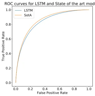
that the input represents either a clicker or buyer session. . . 97 5.3 ROC curves for the LSTM and State of the Art models - on the RecSys

2015 test set. . . 101 5.4 AUC by session length for the LSTM and SotA models, session

quan-tities by length also provided for context - clearly showing the bias to-wards short sequence / session lengths in the RecSys 2015 dataset. . . . 102 5.5 AUC (y-axis) by session length (x-axis) for the LSTM and SotA

mod-els, for any sessions where unrolling by dwelltime was employed. There are no sessions of length 1 as unrolling is inapplicable for these sessions (RecSys 2015 dataset). . . 103 5.6 Model performance (AUC - y-axis) for sessions containing low price

items, split by session length (x-axis) using the RecSys 2015 dataset. . . 103 5.7 Model performance (AUC - y-axis) for sessions containing high price

items, split by session length (x-axis) using the RecSys 2015 dataset. . . 104

5.8 Area under ROC curves for LSTM and GBM models when ported to

the Retailrocket dataset. On this dataset, the LSTM model slightly out-performs the GBM model overall. . . 107 5.9 AUC by session length for the LSTM and GBM models when tested on

the Retailrocket dataset. The bias towards shorter sessions is even more prevalent versus the RecSys 2015 dataset. . . 108 5.10 Strong true positive example: the model correctly has very high

confi-dence (probability = 0.88) that the user has a purchase intention. The items clicked (214601040 and 214601042) also have a higher than av-erage buy likelihood at 6% and 8.1% respectively. . . 111 5.11 Weak true positive example: the model is much less sure (probability

= 0.1) that the session ends with a purchase. The items clicked are not often purchased, so the model has to rely on the day / time of day and price embeddings instead. . . 111 5.12 Strong false positive example: the model incorrectly (probability = 0.98)

classified this session as a buyer. The model was relying on a reason-able item price combined with a time of day when buy sessions are more likely to make its incorrect prediction. . . 112 5.13 Strong true negative example: the model relies on the presence of

un-popular items. For example, item 214842347 occurs only 1,462 times in the entire clickstream (33 million clicks) and is never purchased. . . . 112 5.14 Strong false negative example: this session is a false negative example

(probability = 0.001) - where the session ends with a purchase but our model failed to detect this. This session appears to show an inability of the model to detect long tail buy sessions - sessions containing items that are indeed purchased, but only weakly over the entire dataset. In this example, item 214826912 has a buy:click ratio of 363:21201 or a purchase rate of 1.7%. The corresponding statistics for item 214828987 are 592:23740 and 2.49%. . . 112

6.1 ROC curves for two LSTM models on the RecSys 2015 test set. . . 119 6.2 Training performance of LSTM under two sampling regimes:

chrono-logical (sequential) and random. . . 125 7.1 Following the doctrine in [4], we trained for 1 epoch with an initial rate

of1e−8 and gradually increased this to0.1. The graph clearly intimates values for the minimum and maximum learning rates of5e−5 _and5e−3_{. 132}

7.2 In the 1-cycle policy, the learning rate starts low (1e-4) and increases gradually to1e-3 _{at the mid-way point of the epoch. The rate then cools} again, reaching the original starting point at the end of the epoch. . . 132 8.1 From [5]: Several examples of LSTM cells with interpretable

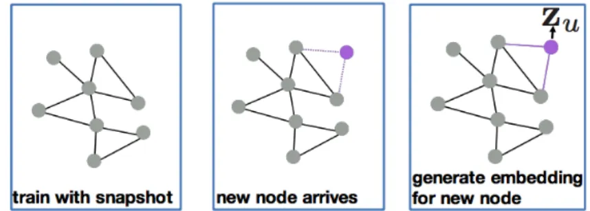
activa-tions discovered when trained on two text datasets - Linux kernel source code and War and Peace. . . 143 9.1 How Graph Convolutional Networks lend inductive capacity to a

trans-ductive model. . . 156 9.2 In generative adversarial networks, two neural networks (the generator

/ poacher and the discriminator / gamekeeper), duel with each other and in doing so mutually improve performance. . . 160

2.1 Sample questions and answers from [6] spanning a selection of common categories. . . 51 2.2 The main model candidates covered in this chapter compared using

re-quirements from the e-commerce domain. . . 57 3.1 A short comparison of the two datasets used - RecSys 2015 and

Retail-rocket. . . 61 3.2 An example of a clicker session from the RecSys 2015 dataset. . . 62 3.3 Examples of the buy events from a buyer session . . . 62 4.1 The top ten session features after training for 7,500 rounds, ordered by

most important features descending. . . 77 4.2 Top ten item features after training for 5,000 rounds, ordered by most

important first. . . 78 4.3 Session and item thresholds by session length with scores for the

cur-rent models, showing the increase in model predictive confidence as the number of events per session grows. . . 80 5.1 Effect of improving different variables on operating profit, from [7].

In three out of four categories, knowing more about a user’s shopping intent can be used to improve merchant profit. . . 85 5.2 Data field embeddings and dimensions, along with unique value counts

for the training and test splits of the RecSys 2015 dataset. . . 94 5.3 Effect of unrolling by dwelltime on the RecSys 2015 and Retailrocket

datasets. There is a clear difference in the mean / median session dura-tion of each dataset. . . 95 5.4 Model grid search results for number and size of RNN layers by RNN

type on the RecSys 2015 dataset. . . 97 5.5 Hyper parameters and setup employed during model training. . . 99 5.6 Classification performance measured using Area under the ROC curve

(AUC) of the GBM and LSTM models on the RecSys 2015 and Retail-rocket datasets. . . 100 5.7 AUC comparisons for n = 30 experiments carried out using random

seeds for the GBM and LSTM models on the Retailrocket dataset. . . . 106 6.1 The effect of sharing hidden layer parameters on four widely used RNN

model architectures - LSTM, GRU, and standard RNN units using TANH or RELU non-linear activation functions. . . 124

6.2 The effect of removing the ability of RNN and LSTM to store dataset statistics other than those directly obtainable from a session (i.e. local) by either freezing embedding weights during training or using simpler, non-gated recurrent units. . . 126

7.1 Model grid search results for number and size of RNN layers by RNN type on the RecSys 2015 dataset. . . 133

Introduction

E-commerce is transforming every avenue of our online lives [8]. Transacting over $2.3

trillion globally in 2017 [9] and growing at an average rate of 10% annually globally,

consumers are increasingly purchasing all types of goods and services online. By

con-trast, many retailers are reporting year-on-year declines in older, physical distribution

channels [8]. The migration is only beginning, with just 3% of global commerce

be-ing conducted online [10]. Since 1995, the capabilities of online retailers have been

driven by parallel advances in all fields of computer science and electronics:

informa-tion retrieval, networking, faster and more scalable hardware have all contributed to the

online explosion. More recently, statistical and machine learning on large datasets has

come to the fore, enabling users to discover content using recommender systems and

search functions to become more relevant. Machine learning holds enormous potential

to further enhance the next wave of e-commerce systems.

1.1

What is E-commerce?

E-commerce is the purchasing of goods and services - both physical and virtual -

on-line. In its earliest form, merchants focused on low-risk items that users were willing

to purchase without seeing them first - books and CDs. From there, online retailing

expanded to include insurance, leisure and business travel, automotive and property.

Today, anything can be purchased online, from fresh groceries to clothing. For

mer-chants, the attraction of online is reduced cost of distribution - fewer physical stores and

sales staff are needed. For users, e-commerce provides convenience, the ability to

com-pare prices and features easily and the flexibility to shop anytime and from any location

with a connection to the internet. Increasingly, machine learning is used to help users

to pro-actively find what they need.

1.2

Evolution of E-commerce

In our opinion, the progression of e-commerce can be divided into five main phases:

1. Infrastructure build out - the creation of the basic software and hardware building

blocks enabling e-commerce (1996 - 1999).

2. Content discovery and search - providing simple search interfaces which exposed

product inventory to users (2000 - 2004).

3. Improved discovery and search - rapid innovation in user interface design and

information retrieval techniques to improve the overall user experience (2005

4. Mobile enablement - supporting the browsing and purchasing of content on

small-screen devices (2010 - 2015).

5. Enhanced functionality using machine learning - modifying system behaviour to

reflect user needs using individual and group user implicit feedback (2015 - now).

The first phase of e-commerce focused on enablement and infrastructure build-out.

Re-tailers invested in basic systems to sell inventory online - relational databases, inventory

management systems and websites - creating supply. Concurrently, datacentres, net-works and ISPs provided connectivity to entire populations to create a complementary

demand. Capacity was grown in parcel delivery services and business processes adapted to cater for the selling of goods online.

The second phase of e-commerce switched focus to providing content discovery tools

to users, along with better user interfaces. Retailers deployed early versions of systems

to guide users to products they are more likely to purchase and to the most popular

content - the Amazon “users who viewed this item also purchased..” feature [11] is a

good example of this. In this phase, most e-commerce systems used SQL to query

rigidly defined database schemas and thus were unable to apply information retrieval

techniques such as gazettes or fuzzy keyword matching to provide a more natural search

interface.

In the third phase, building a better search capability became the focus, resulting in

search engines which provide better search results to users, even when nondescript

terms and phrases are provided. In this phase, a significant overlap developed between

In the fourth phase, mobile device enablement became a key focus, with retailers

de-ploying both HTML and native shopping applications for users. The challenge with

mobile e-commerce is to retain functionality that users expect, when operating on a

constricted budget - screen size, processing power and network access. Users actively

prefer to browse on their mobile device for some e-commerce segments, particularly

where they do not need a large screen and / or have purchased the same item before.

We are currently in the fifth phase of e-commerce - continuing to employ machine

learning to enhance the experience of shopping online, through improvements to

recom-mendations, aids to navigation, personalised user interfaces and much more. Machine Learningdescribes software which learns to improve its performance on a given task over time by minimising an error metric or maximising a reward.

It is important to note that although we have (albeit artificially) time boxed the phases

here, it is entirely possible for some merchants to be far behind the capabilities of others.

In fact this is often the case. Leading retailers like Amazon, Netflix, eBay and Microsoft

have superior capabilities to smaller retailers due to their size, access to development

teams and massive investment in IT and machine learning infrastructure.

Figure 1.1 illustrates elements of this machine learning focus on the user. Individual

panels or tiles are populated by machine learning modules such as recommender

sys-tems or simple statistical calculations such as popular products with a high conversion

Primary / hero offer(s)

Welcome back <<name>>, you have 2 recent orders

Personalised offer 1 Personalised offer 1 Personalised offer 1

Trending offer 1 Trending offer 1 Trending offer 1

FIGURE1.1: Typical organisation for a main or homepage of an e-commerce website.

In this thesis, our focus is on the fifth phase - the intersection of e-commerce with

machine learning to improve outcomes for all participants, both users and merchants.

There are many ways that machine learning can be used to improve the lot of users,

including:

1. Recommender systems - helping users to discover new content based on their

preferences (both implicit and explicit), similarity to other users and content

pop-ularity.

2. Price / product alerts - helping users to change the timing of their purchases to

minimise cost or maximise value, or to know when a scarce item is in stock and

should be purchased.

3. My account functionality (saving preferences, important dates etc. and then

1.3

Current E-commerce Landscape

The advent of e-commerce utterly transformed traditional commerce, and remains

dis-ruptive at its core today - creating new winners and losers as user expectations change

rapidly. The newspaper industry is a good example, with a 50% decline in UK

newspa-per sales since 2005 [13]. People now expect to get their news for free and delivered to

their mobile device on the move - not in a newspaper that they must purchase or have

delivered to one physical location.

Another disruptive e-commerce theme across multiple retail domains is the comparison

website - products that are mostly fungible can be aggregated and compared, enabling

users to save significantly in areas such as insurance, travel, energy supply, mobile

phone contracts and broadband internet [7]. Consumers benefit from this price

trans-parency, and where products are truly fungible and interchangeable e-commerce has

created a more efficient marketplace, but for products that are not fungible or where

post-sales service can be skimped on (or descriptions are less than truthful), the

con-sumer can regret simply purchasing the cheapest option, while more suitable merchants

miss out on sales.

The structure of e-commerce has changed significantly since its inception. Control

of distribution or access to users has coalesced into a small number of portals - for

example Google Shopping, eBay, Amazon and Taobao [14]. Only medium and large

retailers can afford the significant, ongoing investment in e-commerce systems and all

merchants regardless of size, pay very significant marketing and advertising costs to

Twitter Ads. In 2010 [15], an important ruling was passed allowing merchants to bid

for display when competitor brand names, terms and keywords are searched on portals

such as Google. The positive impact of this is that any merchant (as long as they have

sufficient marketing budget) can compete with an established merchant with even the

strongest brand equity and recognition. The negative impact is that overall advertising

costs rise, as more companies compete when bidding for a constrained resource [16, 17].

Large portals face multiple challenges - content discovery, information retrieval and

search results ranking chief among them. Continual advances in information retrieval

have helped, but user sessions are often short both in time and number of interactions,

meaning that portals want to present relevant results quickly - in some cases even

be-fore the user has provided any input. Portals increasingly use recommender systems to

present the best (most relevant) mix of content to users.

These portals can use recommender systems with little downside - but for the merchant

who has no product reviews or ratings, or is not the cheapest, recommender systems can

have a catastrophic effect on trading and profit if they fall foul of the ranking algorithm

[12]. This can occur in two main ways:

1. Popularity bias - the merchant is new or is selling a new product which has no

user reviews or interactions - in this case the new entity is said to suffer from the

cold start problem. Although well-understood and mitigating solutions exist, it

2. Filter bubbles or lack of diversity - where users are only recommended items

or products related to their previous activity. Even popular items which are not

related to previous activity can suffer under this regime.

The current e-commerce landscape then, is one dominated by extremely large portals,

who use a combination of traditional information retrieval techniques and recommender

systems to help users find what they are looking for.

1.4

What’s Missing?

We argue that the online merchants are more often than not ignored by the field of

Computer Science / Software Engineering. As an example, the large research field of

recommender systems is focused on providing end-user utility (for example, suggesting

the best movie to rent or the book we think you will like best) - but not merchant utility

(here is the best customer for you to spend advertising on, here is the optimal price to

set for this product). A large amount of work has been conducted [3, 12, 18] to agree

the best metrics to measure user satisfaction (e.g. dwelltime per item, Mean Squared

Error (MSE), Discounted Cumulative Gain or DCG), but little work has been conducted

to measure merchant or retailer satisfaction.

It can be argued that a satisfied user implies a satisfied merchant but we rebut this. A

happy user is a user who gets the best value deal - their goal is set directly against the

Our focus on the merchant or retailer rather than the end-user is not altruistic, one-sided

or short-sighted. Retailers pay for the e-commerce internet - not end-users and not the

portals. The vast majority of Google’s revenues for example come from merchants who

advertise with Google. If merchants cannot compete or pay too much for advertising and

distribution, then they will go out of business, and competition will reduce, ultimately

resulting in a less efficient marketplace. Consumers will pay more and receive less in

return.

A healthy e-commerce ecosystem requires three sets of actors:

1. Portals / aggregators / agents of discovery.

2. Consumers who use these portals or visit retailers directly.

3. Retailers / merchants who sell or re-sell goods and services to consumers.

Figure 1.2 shows the interplay between the three sets of actors. Consumers can visit

merchant websites directly, but increasingly discover merchants and products via portals

and either purchase directly on that portal (who then claims a distribution or finders fee

from the merchant), or then connect to a merchant. The growth of portals represents

an opportunity and a threat to merchants. While they gain access to larger audiences of

potential customers, they must also pay handsomely for this access. To underline our

earlier point that merchants rely on portals, recently the European Union has opened

an investigation into unfair practices against retailers by one of the most dominant

BP BP BP BP BP

Portals: Amazon, eBay, Google, Facebook, Taobao

Display via advertising

Discover via search

Merchants

Consumers

FIGURE1.2: The primary actors in an e-commerce system and how they interact with each other.

1.5

Practical Impact of Machine Learning for Merchants

As we will see in Chapter 2, there are many different ways in which machine learning

can be employed in the e-commerce ecosystem. Therefore we should consider where

best to apply machine learning in order to address a pressing need that can be

reason-ably implemented. Commercially, merchants care deeply about their cost of advertising.

Large portal owners such as Amazon, eBay, Google, Yahoo, Facebook et al. all already

operate closed advertising systems which they control [16, 17]. However, directly

run-ning optimisation experiments in these environments would be prohibitively expensive,

even though we acknowledge that merchants spend an inordinate amount of their

op-erational budget on advertising. Even the best machine learning model will struggle to

to the contrary, AdWords is naturally run for the benefit of Google, not merchants, and

currently contributes over 85% of Google revenue ($26.6 billion of the $31.1 billion

revenue for Q1 2018) [20].

However, there is one task which can provide valuable input into the following merchant

challenges:

1. Improve bidding strategy (timing, amounts, semantics) on advertising - the largest

single area of operational spend.

2. Improve stocking and product catalogue management - ensuring that popular

items are always in stock.

3. Improve pricing strategy - maximising profit margins where user demand supports

the price and reducing price to grow volume where user demand is weak.

That task is discovering user intent. In information retrieval,intentsignifies what infor-mation the user is searching for based on their queries. Queries can be further segmented

into three main types - informational, navigational and transactional [18].

1.5.1

Problem Statement

In an e-commerce clickstream setting however, we propose a more focused definition

in Equation 1.1:

where:

Sis the set of all user sessions

sis a user session containingnevents{e0. . . en}

ei is a tuple comprised of{timestamp, itemid, itemcat}

T is the set of event types {tc. . . tb}, with tc andtb representing the click and buy event

∀e∈s∈Stest, type(ei) = ec

f is the model implementation (with multiple candidates)

The user intent task is tractable and attractive for a number of reasons:

1. User activity datasets (e-commerce clickstreams) are readily available.

2. Accuracy of user intent prediction is measurable to help refine models over time.

3. Near real-time prediction of user intent represents high-value actionable business

intelligence that merchants can use to only spend time, money and resources on

users who are likely to purchase.

1.6

Proposition

Our proposition is that machine learning can be used in the e-commerce domain for the

direct and measurable benefit of themerchant, and not just the end-user. Merchant ben-efit or utility can be provided in multiple ways - predicting which users are more likely

to purchase than others, assisting the merchant in pricing goods to optimise revenue

and profit. Additionally, we can measure the impact of our proposed merchant benefit

directly, rather than use consumer utility or satisfaction as a proxy measurement.

In order to test our theory, e-commerce datasets containing user activity are required.

Then we will either need to construct good features to correctly classify user intent

or use a technique which can construct a good representation by itself. Our goal is

to use data which is readily accessible and does not violate any privacy legislation or

require private data from end-users. In recent years, research has been conducted on

incorporating multiple signals from social networks into ML e-commerce models [21]

but this approach is increasingly frowned upon and difficult to implement. Users do not

want to share their private data and merchants do not want the overhead of storing and

processing it in a GDPR-compliant (General Data Protection Regulation) manner.

Let us consider a counter-argument to make the previous point clearer and illustrate

the trade-off between persuasion and transparency [22]. Imagine that we constructed a

modelM0 which required the user to log in with their Facebook, Twitter or Instagram

credentials before a search query could be executed in order to provide more relevant

search results (the M0 model uses features which leverage a user’s friend graph and

other private items). Most users would baulk at these requests, even if they believed

that the search results would be better than those provided by a modelM1, which simply

used current, anonymous session interactions.

Lastly, we favour approaches which are straightforward to implement and can provide

1.7

Open Questions

There are three questions that we aim to answer in this thesis:

1. In the user intent discovery task, what is the performance difference between

classic machine learning techniques using explicit features when compared to

deep learning models using a learned representation?

2. What are good representations for e-commerce concepts such as product or user

that can be learned by an appropriate machine learning technique?

3. Can deep neural networks (DNNs) transfer from their traditional applications of

computer vision and natural language understanding to the user intent discovery

task without significant modifications?

1.8

Contribution

Our contribution to these questions is as follows:

1. We conducted a detailed analysis of explicit features showing that four broad

feature classes enable a classic model to infer user intent.

2. We constructed a deep learning model which recovers over 98% of the predictive

3. We show that a standard word language deep model is not optimal for e-commerce

clickstream analysis and propose a combined sampling and hidden state

manage-ment strategy to improve the performance of deep models for the task of user

intent detection in the e-commerce domain.

The work conducted in this thesis was published in the following papers:

1. [23]: Classifying and Recommending Using Gradient Boosted Machines and

Vector Space Models, Humphrey Sheil and Omer Rana, Advances in

Compu-tational Intelligence Systems. UKCI 2017.

2. [24]: Predicting purchasing intent: Automatic Feature Learning using Recurrent

Neural Networks, Humphrey Sheil and Omer Rana and Ronan Reilly, ECOM

workshop at ACM SIGIR 2018.

3. [25]: Understanding E-commerce Clickstreams: a Tale of Two States, Humphrey

Sheil and Omer Rana and Ronan Reilly, Deep Learning Day workshop at ACM

SIGKDD 2018.

1.9

Thesis Roadmap

The following chapters are organised as follows:

• Chapter 2 reviews the current landscape of e-commerce and machine learning to set the scene for our contributary work.

• Chapter 3 sets out the system architecture used to construct, train and benchmark the classic and deep models used in this work.

• Chapter 4 provides a detailed analysis of a particular classic model, Gradient Boosted Machines (GBM), and the importance of different feature classes in the

e-commerce domain.

• Chapter 5 constructs and benchmarks a competing deep learning model with fur-ther sections focused on model interpretability and model comparison.

• Chapter 6 explores how standard deep word-based language models must be mod-ified to function effectively in the e-commerce domain for the user intent

discov-ery task.

• Chapter 7 reviews our hyperparameter tuning efforts.

• Chapter 8 provides a critical assessment of our work and places it in context to existing work.

• Chapter 9 previews suggested future work and summarises the thesis contribution.

1.10

Summary

E-commerce is a domain where machine learning has already been applied successfully,

but much remains to be done - in particular, serving the needs of merchants more fairly

In addition, the selection of a target e-commerce problem in practice also depends on

the availability of good data, the opportunity to directly impact and measure the

perfor-mance of the machine learning model and ideally, a computationally fast model which

can generate outcomes in near real-time to be effective in an e-commerce context. In

the next chapter, we will set out a short overview of machine learning and how it is

Background and Related Work

In our opinion, the intersection of e-commerce and computer science is an area of active

research for a number of reasons:

1. Clear, significant commercial interest - e-commerce is a real world problem with

immediate applicability.

2. The ready availability of datasets suitable for analysis - from user activity logs to

product catalogues.

3. A well-defined mechanism (A/B testing) to test new implementations and theories

in an online and offline setting.

The diagram below illustrates the broad anatomy of an e-commerce website from a user

/ functional perspective. We use this diagram to ground our further discussion of how

machine learning is currently used across this structure.

Recommendations

Navigation

Search

Intent prediction

Homepage

Shopping basket

Product / item landing pages

Category landing pages

Review order page

Order confirmation page

Machine

learning

services

User

destinations

FIGURE2.1: Broad anatomy of an e-commerce website from an end-user perspective, providing a reference map for future discussions on how ML is applied to e-commerce.

2.1

Background

In the following sections, we provide an overview of machine learning, in order to

ground our overview of how it is used in e-commerce currently, and to inform more

2.2

Machine Learning

Machine Learning precedes the field of e-commerce significantly - and if we include

statistics as a natural complement / pre-cursor to machine learning, the joint fields are

older still.

E-commerce is an ideal domain in which to train and deploy machine learning models

since good datasets are common and relatively easy to gather, while tasks are often

automated. For example, it is the norm for user sessions to be modelled as a tuple of

{userid−eventtype−itemid} and for these tuples to be grouped into user sessions based on a maximum time window (for example 30 minutes). Web server logs are

regularly processed to extract these datasets and these datasets can then be fed into

multiple machine learning model candidates.

In Chapter 1 we stated that machine learning (ML) represented a class of software which

can learn to improve its own performance from past experience. Figure 2.2 illustrates

the primary or basic components of any machine learning system.

A minimal ML system consists of [26]:

1. A dataset - the input dataset with either output target labels (desired outputs) or

target mappings.

2. A model - the abstraction of the problem to be solved, or the mathematical

Input data

Model

Task

Error

Output

Representation learning / feature engineering

FIGURE2.2: The primary components of a supervised machine learning system where

we have labelled data and thus can calculate an error as the difference between the expected and actual output from the model.

3. A loss or error function which measures the difference between the actual model

outputs and desired outputs (we assume that our data is labelled and thus we are

training in a supervised setting).

4. A training or optimisation algorithm - using the loss function to modify the model

in some way so that future iterations provide better outputs for the task at hand.

Each of these items may be considered as a pluggable component where the

imple-mentation can be replaced to best fit specific needs (simplicity, speed, scalability,

2.2.1

Datasets

The input data, combined with the task we wish our model to learn, affects the

selec-tion of all other components in the ML system. Data can be virtually anything - from

images to video, audio, handwriting and so on. For the scope of this thesis however, the

datasets under consideration are e-commerce-related clickstreams, and thus are

over-whelmingly structured text. In addition, we can make the following generalisations

about e-commerce clickstreams:

1. They are large - typically with millions of entries or samples to consider.

2. They are heavily imbalanced - the class label or target we are interested in (buyers,

fraudsters) is far smaller than the dominant label (clickers, non-fraudsters).

3. Time plays an important role - users spend time dwelling on items, user sessions

have a length measured in events and time, and the entire dataset can often be

considered and processed as a time series.

2.2.2

Models

There are many types of model implementations available. While there is no single

agreed taxonomy to organise all of the model families, the following categories are

proposed in [26]:

1. Linear models.

3. Distance-based models.

4. Probabilistic models.

In the following sections, we focus on the subset of models relevant to the user intent

discovery task.

2.2.3

kNN - k Nearest Neighbours

kNN is an example of a distance-based model. It is simple to train - the model iterates

over and memorises the training data. Then at inference time a certain number -k ≥1 - of the points closest to the input data are used to vote and predict the majority class.

A variety of distance metrics (e.g. euclidean distance, Jaccard index, cosine similarity)

are used depending on the input data to create clusters of similar exemplars.

The training data consists of feature vectors xi and label pairs yi for each example

(x1, y1),(x2, y2), . . . ,(xn, yn) and training time is fast - O(n) while inference

perfor-mance at run-time is slow - alsoO(n), since all examples need to be compared to the inputxito find the closestkmatches. kNN models have high variance since the decision

regions of the model are created directly from the training data.

2.2.4

Gradient Boosted Machines / Decision Trees (GBM / GBDT)

Tree models are very popular in Machine Learning - high quality implementations exist

. . .

FIGURE2.3: In GBDT, each tree is a weak learner, and when combined these separate trees form a single strong learner.

than other black box approaches (although complex trees or collections of trees are

certainly more difficult to understand). Decision trees used in data mining are of two

main types:

1. Classification tree analysis - used when the desired outcome is to predict the class

to which the data belongs.

2. Regression tree analysis - used when the predicted outcome can be considered a

real number (e.g. the price of a house, or a patient’s length of stay in a hospital).

The term Classification And Regression Tree (CART) analysis is an umbrella term used

to refer to both of the above procedures [26]. As their name suggests, trees are made up

of nodes which representtests of supplied features(for example, test if dwell time >

100) and edges which control the path to be followed based on the outcome of these

tests.

Trees used for regression and trees used for classification have some similarities but also

some differences, such as the procedure used to determine where to split. Ensemble

methods construct more than one decision tree: boosted trees incrementally build an

ensemble by training each new instance to emphasise the training instances previously

Gradient Boosted Decision Trees (GBDT) do exactly this and attempt to iteratively

minimise theresidual error, i.e. the error remaining after the most recent tree (weak learner) has been added to the current ensemble. Figure 2.3 illustrates the concept

of additive trees which combine to form a single strong learner. We use colours to

illustrate that the individual trees constructed vary by structure and features used, and

are combined to minimise the overall error.

Different implementations of GBDT [27–29] use different heuristics and optimisations

to build trees (for example handling categorical variables differently, adding a

regular-isation term and / or favouring simpler trees to guard against overfitting) but all

imple-mentations share a common goal: at each iteration, minimise the remaining residual

error. Regardless of the implementation chosen, the performance of the trained model

is heavily reliant on the quality of the supplied feature set.

GBM / GBDT hold multiple state of the art benchmarks in e-commerce and we

investi-gate the performance of GBM in detail on the user intent discovery task in Chapter 4.

2.2.5

Markov Chains / Hidden Markov Models

Markov chains and their derivative - hidden Markov models, are both examples of

abilistic machine learning models. A Markov chain is a model that represents the

prob-abilities of sequences of random variables. The central assumption in a Markov chain is

s

1

s

2

a

12

s

3

s

4

y

1

y

2

b

4

(

y

2

)

FIGURE 2.4: This example HMM with 4 states can emit 2 discrete symbolsy1 ory2.

aij is the probability to transition from statesi to statesj. bj(yk)is the probability to

emit symbolykin statesj.

states prior to it. Figure 2.4 illustrates a very simple 4-state HMM. In this constrained

HMM, states can only reach themselves or their adjacent (prior and subsequent) state.

A hidden Markov model (HMM) is an extension to the standard Markov chain where

some events of interest are hidden or not directly observable. Chapter 8 of [3] (3rd

edition, currently under construction) provides standard terminology for Markov chains

and models as follows:

S =s1, s2, . . . , snA set ofN states

A = a11, a12, . . . , an1, . . . , ann a transition probability matrix A, each aij

representing the probability of moving from stateito statej

π = π1, π2, . . . , πN an initial probability distribution over states. πi is the

probability that the Markov chain will start in state i.

At first glance, HMMs seem like an ideal candidate to construct a model of user

interpretable - much like probabilistic graphical models [30]. Moreover, they can

ac-commodate inputs of variable length so can model clickstreams naturally. However,

they suffer from some limiting drawbacks [31]:

1. They cannot express dependencies between hidden states - therefore long-range

correlations or connections cannot be modelled by a single HMM. In fact, only a

small subset of possible sequences can be modelled by a reasonably constrained

HMM.

2. HMMs model discrete states, and exclude the possibility of encoding other states.

3. If states should depend on multiple states, then the number of states increases rapidly, e.g. N2_{states are required if each state depends on two states.}

In direct contrast to HMMs, neural network models (see below) can capture and model

continuous states which is a meaningful advantage. Empirically, a specific type of

neu-ral network model (Long Short Term Memory which we will cover in detail in

Chap-ter 5) began to outperform HMM in the domain of speech recognition in 2012 [32] and

since then in multiple other domains.

In [31], the concept of hybrid HMM - neural network models are proposed to combine

the best of both models however it is fair to say that there is still much work to be

done in this area. Much later in Chapter 8 we will cover a related concept to HMMs

- causal inference - which aims to provide interpretable, more powerful models which

2.2.6

Neural Network Models

Artificial Neural networks (ANNs) and in particular Deep Neural Networks (DNNs)

are well suited to problems that are non-linear and where the data contains nuances

and patterns not readily obvious to a human. Put another way, deep feedforward neural

networks are associated with complicated, non-convex objective functions that simpler

models cannot solve or approximate.

Artificial Neural Networks are complex, nonlinear and parallel computers composed of

very simple computing units or neurons. A neuron receives signals from other neurons,

combines them and depending on some threshold and an activation function, will either

fire or not. Neurons are organised in layers - input, hidden and output layers. Input

layers directly receive input data, output layer values are the final values from the

net-work after all processing has completed. Hidden layers are not strictly speaking hidden

- their values can be examined at any point during training or inference, but what they

are processing, i.e. the abstractions coded into one or more hidden layers, is always

open to interpretation, hence the name.

Figure 2.5 illustrates the canonical view of a simple neural network.

We note that neural networks fell dramatically out of fashion from 1989 - 2009,

primar-ily as a result of overpromising - the so-called (second) AI winter. They came back into

vogue from 2010 onward due to the proliferation of large datasets and highly parallel

Input #1

Input #2

Input #3

Input #4

Output

Hidden

layer

Input

layer

Output

layer

FIGURE 2.5: A simple neural network. Units are divided into three types (input, hid-den, output) and organised into layers. In this example the network is fully connected

in a feedforward manner.

2.2.6.1 Deep Neural Networks

Since 2010 deep neural networks (DNNs) [33, 34] hold state of the art performance on domains such as language translation, handwriting recognition and varied computer

vision tasks including sequence to sequence translation [35] (relevant for clickstream

analysis). DNNs are closely related to ANNs, and it is largely the joint advent of a

hardware architecture (general purpose GPU or GPGPU) and open datasets such as

MNIST and ImageNet that enabled DNNs to achieve their performance.

The exact meaning of deep in DNN is not defined, but colloquially most researchers take it to mean 10 or more hidden layers. DNN variants such as Highway Networks

[36] can have hundreds of layers. Figure 2.2.6.1 shows the deep model from Microsoft

trend throughout the ImageNet competition was the increase in number of layers used,

from GoogLeNet, AlexNet and finally ResNet.

FIGURE2.6: The winner of the 2015 ImageNet competition from Microsoft Research

- ResNet [1], depicted alongside the VGG19 model.

DNNs must be trained in order to work effectively, and it is backpropagation combined

with gradient descent that is most often used to train DNNs. In supervised learning

back-propagation can be seen as the chain rule applied to the error derivatives from

y w1 w2 w3 Hidden layer Input layer Output

layer _{(a) Forward Pass}

y = φ X

i

wixi

!

(b) Error at the Output

E = 1₂(t− y)2

(c) Backward Pass

∆wi = −η_δwδE

i

FIGURE2.7: From [2]. Overview of backpropagation.

reverse passes are combined using back-propagation and stochastic gradient descent

to train a network. To start, a training pattern is fed forward, generating corresponding

output. Next, the error between actual and desired output is computed. Finally, the error

propagates back through the network, through updates where a ratio of the gradient (_δwδE

i)

is subtracted from each weight. xi, wi, Φare the inputs, input weights, and activation

function of a neuron. ErrorE is computed from outputyand desired output or targett.

ηis the learning rate.

Due to the large number of parameters, DNNs are particularly susceptible to overfitting,

and can create models which are brittle or behave badly when presented with mildly

perturbed or unexpected data - for example samples never seen before during training,

or samples drawn from a slightly different distribution [37].

A wide range of countermeasures have been designed to address overfitting, including

2.2.6.2 Recurrent Neural Networks

Recurrent neural networks [40] (RNNs) are a specialised class of neural networks for

processing sequential data. A recurrent network is deep in timerather than space and arranges hidden state vectorshl_tin a two-dimensional grid, wheret= 1. . . T is thought of as time and l = 1. . . Lis the depth. All intermediate vectors hl

t are computed as

a function of hl

t−1 and h

l−1

t . Through these hidden vectors, each output y at some

particular time steptbecomes an approximating function of all input vectors up to that time,x1, . . . , xt[5]. We will see RNNs in more detail in Chapter 5.

2.2.6.3 Embeddings

Neural networks typically deliver their best performance not when consuming explicit

hand-crafted features, but instead learning the best representation through training.

In this regime, concepts in the input data (for example items or categories in the

e-commerce domain) are modelled as words and each word is then transformed into a

low-dimensional distributed representation - the embedding or word vector [41]. A

good vector space model will map semantically similar words close together. We will

cover embeddings in more detail in Chapter 5.

2.2.7

Loss / Objective Functions

A loss provides a numerical measure of the difference between the desired output of

a model and the actual output. Although this may sound obvious, it is a fundamental

objective function and this name gives a truer account of its purpose - it is measuring

the ability of a model to carry out the task asked of it. In other words, it is framing the

learning component.

Intuitively, we want outputs that are more different to be penalised more, and actual

outputs that are closer to desired outputs to be penalised less. The loss is then used to

update the model in some way by the training algorithm - the essential part of machine

learning.

2.2.7.1 Categorical Cross-entropy

The categorical (also known as multinoulli) distribution is aK class generalisation of the two class Bernoulli [42]. Generally the prediction is a vector of probabilities for

each class, so the targetyt is a class in the one-hot representation as a vector of length

K, k = 0. . . K, whereK is the number of classes. We will see this particular loss in more detail in Chapter 5.

2.2.7.2 Auxiliary Losses

In deep learning, a useful augmentation to a primary loss is to augment it with another

associated loss - the so-called auxiliary loss. The immediate effect of this is to increase

the size of the loss and thus the size of the gradients and in some cases this can

ame-liorate the vanishing gradient problem, especially in a sequence processing setting with

2.2.8

Training and Optimisation

The process of training an ML model involves providing an ML algorithm (that is, the

learning algorithm) with training data to learn from. The term ML model refers to the

model artifact that is created by the training process. Some models are created before

training, in particular deep learning models, while some training algorithms create the

model architecture from the training data e.g. Gradient Boosted Machines (GBM).

Different regimes of machine learning are clearly discernible - supervised, semi-supervised

and unsupervised, but in all cases the goal of training a machine learning model is to

provide the model with example data so that it learns to minimise some error metric (or maximise some reward if reinforcement learning is used) and then to generaliseto unseen data.

In a supervised setting where labels are known, training is most often implemented as

gradient descent, for example Stochastic Gradient Descent or SGD. Various

enhance-ments have been proposed for gradient descent, including Nesterov momentum etc.

Although it may seem obvious that the goal of gradient descent is to find a global

min-imum in the gradient landscape, i.e. co-ordinates where the overall error is lowest, in

practice this is not the case - in fact a global minimum would represent significant

over-fitting on the training set, preventing good generalisation tounseendata and the over-trained model would perform poorly in practice. Techniques such as dropout [38, 43],

L1 and L2 regularisation have also been developed to guard against overfitting. In fact,

2.2.9

The Bias-Variance Tradeoff

Updating a model during training to minimise a specified error (for example mean

squared error) is a key step in machine learning. Models are affected by three types

of error [44]:

• Bias - aka underfitting, where the model cannot associate between features and outcomes.

• Variance - aka overfitting, where the model cannot generalise from the training set to unseen data.

• Noise - or the irreducible error (unpredictable changes or measurement errors), which cannot be explained by any model.

The bias-variance trade-off essentially states that we can have a model with no bias or

no variance, but not both. Combining the three terms as per [45] we can see in equation

2.1:

E(y0−fˆ(x0))2 =V ar( ˆf(x0)) +Bias( ˆf(x0))2 +V ar() (2.1)

where:

E = the error or difference between target and actual value

x0 = a given value ofX y0= target value for inputx0

V ar()= the irreducible error or noise in the dataset ˆ

f(x0)= actual value for inputx0 produced by the model.

We can minimise (but not eliminate) bias and variance through the selection of an

ap-propriate training regime and training data. In addition, in some cases it may make

sense to train a biased model or estimator if our goal is to minimise the mean squared

error.

2.3

Machine Learning In E-Commerce

Now that we have provided an overview of machine learning, in the following sections

we propose how machine learning is used in, and influences the field of e-commerce as

follows:

1. As a common, visible service - used to improve the end-user experience directly,

e.g. recommendations, predicting user intent, learning to rank.

2. As a common, invisible service - used to improve the end-user experience

indi-rectly, e.g. catalogue management, fraud detection.

3. As an important e-commerce ecosystem service - for example predicting

click-through rates.

Our aim is to show the breadth and depth of the e-commerce domain, coupled with the

pervasive application of machine learning throughout the domain. An important point

on very large datasets and produce predictions on unseen data in near real-time. Dean

and Barroso provides an insight into the varied techniques used to ensure that virtually

all users are happy with system performance even at massive scale.

2.4

Predicting Ad Click-through Rates

Given that the dominant business model of the web is offering a free service

comple-mented by monetisation through advertising, it comes as no surprise that predicting and

increasing click-through rates has received a lot of research attention [47, 48].

Predict-ing ad click–through rates (CTR) is a massive-scale learnPredict-ing problem that is central to

the multi-billion dollar online advertising industry.

2.5

Content Discovery

Content discovery is one of the older applications of ML to e-commerce [11]. In this

use-case, the merchant or portal has far more content than the user can browse through

manually, or has noticed that users have low session time / high churn rates on the

service. Recommender systems [12] are widely used to predict what content or product

the user will be interested in based on their previous behaviour. Within the field of

recommender systems, a wide variety of machine learning techniques are employed to

achieve this goal, such as:

1. Statistical analysis (popularity) - this is often used in the cold start setting, where

2. User similarity and item similarity using approaches such as matrix factorisation

[49].

3. Sequence processing using recurrent networks [50].

If unsolved, the user - content mismatch typically manifests in a number of ways, all

detrimental to the overall user experience and hence site popularity and ultimately

prof-itability [12]:

1. User paralysis - the sheer number of options cause the user to freeze and never

consume content [11].

2. The needle in the haystack - the user cannot find what they are looking for, either

by searching or navigation [11].

Recommender systems are designed to directly address this problem, by proposing

con-tent or products to users, after observing only a very small number of interactions or no

interactions at all (the so-called cold start problem). In some domains, recommender

systems work very well, for example 75% of all content consumed on the Netflix

plat-form comes from their various recommendation algorithms. From figure 2.1 we can

see that recommendations are commonly used across an entire e-commerce website - to

suggest new content, up-sell and cross-sell.

However, recommender systems also suffer from a number of drawbacks [51].

Feed-back loops caused when training data is harvested from a production deployment where

measures such as low diversity of recommendation, high homogeneity of users and the

ability to create filter bubbles are well-known issues in the recommender community.

2.6

Predicting purchase propensity

Knowing what a user intends to do clearly has value. Search results can be made more

relevant, concrete calls to action can be targeted towards the user to help them discover,

browse or purchase new content or to persuade them to complete their purchase.

Most of the data used to infer user intent isimplicit, not explicit. It is difficult to get users to give feedback on their site experience, so instead we use their known behaviour

(i.e. their clickstream) to infer it. Joachims led the way in using implicit signals in the

form of clickthrough data to re-rank documents returned for a given query so that the

most relevant entries are at the top of the list. In this work, a Support Vector Machine

(SVM) was used to implement the ranking algorithm. Although the main purpose of

[52] is to improve the ranking function for a search engine, it is also inferring user

intent from implicit signals, as it is only when user intent is known that more relevant

results can be prioritised. Inferring user intent can also be situated as a special case of

personalised search. In [53], the authors utilise variability in user intent as measured

by several click-based measures (click entropy, potential for personalisation curves) to

show that different users will find different results relevant for the same query.

Another line of work relevant for user intent is change point detection in user

prefer-ences over time. In [54], Hidden Markov Models (HMM) are used to identify these

using clickstreams as a proxy for user intent, i.e. an implicit signal. This is a concept

that we leverage heavily in the future chapters.

Forecasting whether or not a user will purchase an item is closely related to, but separate

from that of predicting content interactions. For example if user uk clicks on itemim

and we know that im is both popular and frequently purchased, this allows our model

to be more confident in predicting thatukhas a higher propensity to purchase than the

median or mean.

But many more local and global variables also need to be taken into account - the user’s

dwelltime or think time per item, the time of day and season, what other users are

currently doing on the site, merchant sales events or special offers [12, 55, 56].

However, the investment involved is worth it to the merchants and portals. Specific

actions can be directed to potential buyers to convince them to commit: targeted

adver-tising, special incentives such as time-limited discounts and so on.

The problem of user intent or session classification in an online setting has been heavily

studied, with a variety of classic machine learning and deep learning modelling

tech-niques employed. [55] was the original competition winner using one of the datasets

considered in later chapters using a commercial implementation of GBM with extensive

feature engineering and is still to our knowledge the state-of-the-art implementation for

this dataset.

Hidasi et al. uses RNNs on a subset of the same dataset to predict the next session

click (regardless of user intent) so removed 1-click sessions and merged clickers and

[58] compares [57] to multiple models including kNN, Markov chains and association

rules on multiple datasets and finds that performance varies considerably by dataset.

[59] extends [57] with a variant of LSTM to capture variations in dwelltime between

user actions. User dwelltime is considered an important factor in multiple

implementa-tions and has been addressed in multiple ways. For shopping behaviour prediction, [60]

uses a mixture of Recurrent Neural Networks and treats the problem as a

sequence-to-sequence translation problem, effectively combining two models (prediction and

rec-ommendation) into one. However only sessions of length 4 or greater are considered

- removing the bulk from consideration. From [61], we know that short sessions are

very common in e-commerce datasets, moreover a user’s most recent actions are

of-ten more important in deciphering their inof-tent than older actions. Therefore we argue

that all session lengths should be included. [62] adopts a tangential approach - still

focused on predicting purchases, but using textual product metadata to correlate words

and terms that suit a particular geographic market better than others. Broadening our

focus to include the general use of RNNs in the e-commerce domain, Recurrent

Rec-ommender Networks or RRNs are used in [50] to incorporate temporal features with

user preferences to improve recommendations, to predict future behavioural directions,

but not purchase intent. [63] further extends [57] by focusing on data augmentation and

compensating for shifts in the underlying distribution of the data.

In [64], the authors augment a more classical machine learning approach (Singular

Value Decomposition or SVD) to better capture temporal information to predict user

behaviour - an alternative approach to the event replication or unrolling methodology

Using embeddings as a learned representation is a common technique. In [65],

em-beddings are used to model items in a