Chalmers Publication Library
Initializing Wiener–Hammerstein models based on partitioning of the best linear
approximation
This document has been downloaded from Chalmers Publication Library (CPL). It is the author´s version of a work that was accepted for publication in:
Automatica (ISSN: 0005-1098)
Citation for the published paper:
Sjöberg, J. ; Schoukens, J. (2012) "Initializing Wiener–Hammerstein models based on partitioning of the best linear approximation". Automatica, vol. 48(2), pp. 353â359.
Downloaded from: http://publications.lib.chalmers.se/publication/154346
Notice: Changes introduced as a result of publishing processes such as copy-editing and
formatting may not be reflected in this document. For a definitive version of this work, please refer to the published source. Please note that access to the published version might require a
subscription.
Chalmers Publication Library (CPL) offers the possibility of retrieving research publications produced at Chalmers University of Technology. It covers all types of publications: articles, dissertations, licentiate theses, masters theses, conference papers, reports etc. Since 2006 it is the official tool for Chalmers official publication statistics. To ensure that Chalmers research results are disseminated as widely as possible, an Open Access Policy has been adopted. The CPL service is administrated and maintained by Chalmers Library.
Initializing Wiener-Hammerstein Models Based on
Partitioning of the Best Linear Approximation
J. Sj¨
oberg
aJ. Schoukens
ba
Chalmers University of Technology, Department of Signals & Systems, SE412 96 Gothenburg, Sweden. b
Vrije Universiteit Brussel, Faculty of Engineering, Department of Fundamental Electricity and Instrumentation, Pleinlaan 2, 1050 Brussels, Belgium
Abstract
This paper describes a new algorithm for initializing and estimating Wiener-Hammerstein models which consist of two linear parts with a static nonlinearity in between. The algorithm makes use of the best linear model of the system, which is a consistent estimate of the systems dynamics for Gaussian excitations. The linear model is split in all possible ways into two sub-models. For all possible splits, a Wiener-Hammerstein model is initialized which means that a nonlinearity is introduced in between the two sub-models. The linear parameters of this nonlinearity can be estimated using least-squares. All initialized models can then be ranked depending on the fit. Typically, one is only interested in the best one, for which all parameters are fitted using prediction error minimization.
The paper explains the algorithm in detail and consistency of the initialization is proven. Computational aspects are investigated, showing that in most realistic cases, the number of splits of the initial linear model remains low enough to make the algorithm useful. The algorithm is illustrated on an example where it is shown that the initialization is a tool to avoid many local minima.
Key words: Wiener-Hammerstein systems, Hammerstein systems, Wiener systems, nonlinear system identification
1 Introduction
There has always been a need to identify nonlinear sys-tems using measured data. In real life all syssys-tems are nonlinear to some extent but linear system theory and linear system identification methods have often been successfully applied. Theory for linear system identifica-tion is a fairly mature area, well covered in books like, eg, [11, 19], focusing on time domain methods and [12], focusing on frequency domain methods.
During the last two decades there has been a growing in-terest to go beyond linear identification and to identify real nonlinear models of the nonlinear systems. General model structures, like Volterra expansions, or different types of neural network expansions which can approx-imate “almost” any nonlinear relations have been pro-posed and investigated extensively in the literature, see, eg, [18] for an overview. The drawback using very flexible models is an increased risk of a high variance
contribu-Email addresses: [email protected]
(J. Sj¨oberg),[email protected] (J. Schoukens).
tion to the model error and problems with the “curse of dimensionality”. The papers [8, 18] explains these prob-lems and presents some remedies.
One approach to avoid the problems with the flexible, general, model structures is to work with block-oriented nonlinear models built up by combining blocks which are either linear dynamic or static nonlinear. By constrain-ing the dynamics to be linear one can also use part of the linear system theory and analysis of the model proper-ties become easier. The simplest block-oriented models are the Hammerstein model and the Wiener model where the Hammerstein model consists of a static nonlinearity followed by a linear dynamic block. The Wiener model has the two blocks in the reversed order. These mod-els can be generalized into Hammerstein-Wiener modmod-els, which has two static nonlinear blocks with a linear dy-namic block in between, and Wiener-Hammerstein mod-els with two linear blocks with a static nonlinear block in the middle, see Figure 1.
With the introduction of a block structure, the need, and possibility, for tailored estimation methods follows. This papers presents a novel consistent algorithm for
es-G1HqL G2HqL
uHtL y`HtL
Fig. 1. A Wiener-Hammerstein model structure.
timating Wiener-Hammerstein models. In the literature, many approaches for estimating block-oriented models have been published. Early results can be found in [1] and [3]. The first one of these also contains many refer-ences to pioneer works. A stochastic embedding of the estimation problem is given in [4] and the maximum likelihood estimate is formulated. Recursive estimation of MIMO Wiener-Hammerstein models is investigated in [2].
A key problem in identifying Wiener-Hammerstein mod-els is the initial estimates of the two linear blocks, in-cluding the degree of them. While initialization and esti-mation methods exists for the simpler block models, see eg [16,20–22] for Wiener models, and [7] for an overview of Hammerstein models, there is a lack for of these for general Wiener-Hammerstein models. In [5] an iterative initialization procedure is proposed which requires spe-cially designed periodic excited input signals. This ex-perimental requirement is relaxed in [15].
In [23] random, stable, initialization of the two sub-systems is investigated with quite good results. The au-thors show that there are many local minima, so, typi-cally, the estimation needs to be repeated several times with different starting values to increase the chances of finding a model corresponding to a good local minimum. In this paper a novel algorithm is proposed which is based on the Best Linear Approximation (BLA) of the nonlinear system. That means that the algorithm starts with linear identification to obtain the BLA model. Under some mild assumptions, see Section 4, the BLA model will be a consistent estimate of the concatenated dynamics of the two linear sub-systems. The core idea of the algorithm is then a brute-force approach, sim-ply splitting the BLA model into two sub-models in all possible ways, initialize a Wiener-Hammerstein model with each one of these splits, and then choose the best initialization. The contributions of the paper are the consistency of the algorithm and that the initializations can be formulated as least squares (LS) problems which makes it feasible up to model orders of approximately 10. The consistency result means that problems with lo-cal minima are avoided which cannot be guaranteed by any other suggested algorithm for this model structure. The idea to base the initial Wiener-Hammerstein model on the BLA model is not new. In, for example, [9] an algorithm is given where initially the entire BLA model is put on both sides of the nonlinearity.
The paper is organized as follows. Section 2 details the problem formulation and the proposed algorithm is
pre-sented in Section 3. The consistency of the algorithm is shown in Section 4. Sections 5 and 6 concern the com-plexity and the computational burden for the algorithm. In Section 7 the algorithm is illustrated on an example and the paper ends with conclusion in Section 8.
2 Problem Formulation
The problem formulation is divided into three steps, the definition of the model structure, the assumptions on the data, and the definition and computation of the es-timate.
2.1 Model structure
The concerned model structure is of Wiener-Hammers-tein type described by
z(t) =G1(q−1, α)u(t)
x(t) =f(β, z(t)) (1) ˆ
y(t, θ) =G2(q−1, γ)x(t)
where ˆy(t) is the model’s prediction of the outputy(t), andG1(q−1, α) andG2(q−1, γ) are linear time invariant
transfer functions in the delay operatorq−1, and
param-eterized with αand γ, respectively. In the sequel, the arguments of the transfer functions are sometimes omit-ted to simplify the notation. The function f is a static nonlinearity parameterized withβ. All parameters of the model structure are stored in a common parameter vec-tor
θ= [α, β, γ]. (2) The first linear part of the model can be described as
G1(q−1, α) = b1 0+b11q−1+· · ·+b1mb1q −mb1 1 +a1 1q−1+· · ·+a1ma1q −ma1 (3) whereα= [b1 0, . . . , b1mb1, a 1 1, . . . , a1ma1] , andG2(q −1, γ) is
described similarly withγ= [b2
0, . . . , b2mb2, a
2
1, . . . , a2ma2]. The static nonlinearity is described as a basis function expansion f(β, z) = n X k=1 βk1fk(β2k, z) (4) β= [β1, β2]T = [β11, . . . , βn1, β12, . . . , βn2]T
wherefkare basis functions, andβhas been divided into
β1, which enters linearly inf, andβ2, which can contain
several parameters, and which enters non-linearly inf. With this general description of the static nonlinearity most specific basis function expansions can be described
with a specific choice of the basisfk. If, for example, a
polynomial model is chosen, then
f(β, z) =β01+β11z+β21z2+. . . βn1zn
and in this case there are no parameters inβ2.
To define a model in this model structure, not only the parameters need to be determined but also the orders of the sub-models, and the type of basis function expansion inf.
2.2 Data
For the estimation of the parameters in the model (1) a data set is assumed to be available,{u(t), y(t)}N
t=1ofN
inputu(t) and outputy(t) samples.
The data generating process does not need to be of the form (1), but when consistency is studied in Section 4 it is assumed to be so, with a slightly more general as-sumption on the nonlinearity. In that case, it is impor-tant to notice that the intermediate variablesz(t) and
x(t) are not available. Also, for the consistency it is as-sumed that the input signalu(t) is Gaussian.
Otherwise rather mild conditions are needed on the data like the one in [10] for the algorithm to be applicable.
2.3 Computing Estimation
A standard prediction error approach is assumed to be used to define the estimate ˆθNof the parameter vectorθ
for the model (1) based on the data set{u(t), y(t)}N t=1.
It is based on minimizing the prediction error
ε(t, θ) =y(t)−yˆ(t, θ), (5) the difference between the measured outputy(t) and the prediction with (1),
ˆ
y(t, θ) =G2(q−1, γ)f(β, G1(q−1, α)u(t)). (6)
This is done by using a criterion of fit
VN(θ) = 1 N N X t=1 ε2(t, θ) (7) and then defining the estimate as
ˆ
θN= arg min
θ VN(θ). (8)
The estimate (8) is computed with a gradient based it-erative algorithm. Given a start valueθ(0), iterate
θ(i+1)=θ(i)−RidVN(θ)
dθ (9)
until convergence. The matrixRiis to modify the search
direction and step size to assure downhill steps. Depend-ing on how Ri is chosen (9) describes a wide class of
well-known standard algorithms like the Gauss-Newton and the Levenberg-Marquardt algorithms. Also the al-gorithm used in [23] can be obtained by choosingRito
be the Gauss-Newton approximation with some of the smallest eigenvalues truncated.
All three blocks of the model structure (1) contain a gain parameter, and two of them are typically fixed in the iterative minimization, eg,b1
0andb20.
In the example in Section 7 a Levenberg-Marquardt al-gorithm is used to compute the minimization. A soft-ware package for the Mathematica platform, [17], has been used which has the advantage that when the model structure (1) has been defined, all expressions needed in (9) to apply the Levenberg-Marquardt algorithm are cal-culated automatically. The symbolic features of Math-ematicaare used to automatically generate expressions for the derivatives. The symbolic expressions are also simplified so that, eg, multiple identical expressions are only calculated once.
Typically,VN(θ) can have many minima and the success
of the minimization depends on the initial estimateθ(0).
The contribution of this work is a novel algorithm to compute this initial estimate.
3 Proposed Algorithm
The algorithm consists of the following steps. Algorithm 1
1. Start with the best linear modelG(q−1).
Only the plant model is of interest. One can, hence, con-strain to evaluate output error models. If Box-Jenkins models, or ARMAX models are used, only the estimated plant model is retained. Also frequency domain meth-ods can be used to obtain the model. In that case a non-parametric noise weighting can be used to improve the quality of the initial estimate.
2. Split the linear model into all possibleG1(q−1) and G2(q−1) so thatG(q−1) =G1(q−1)G2(q−1).
To do this, poles and zeros of the linear model need to be calculated. These are then divided in all possible ways into to sub-modelsG1andG2. Depending on prior
knowledge of the system, some of the divisions can be excluded. This is discussed in Section 5.
3. For all partitions of the linear model,{G1, G2}, use u(t) andG1 to decide values forβ2 and then LS to
fit the linear parameters, β1, in the nonlinearity as
initialization.
The position parametersβ2 for the basis functions are
decided using the distribution of the input to the non-linearity{z(t) =G1(q−1)u(t)}Nt=1.
Minimizing (7) with respect to the parametersβ1in (4)
is straightforward by first writing (6), ˆy(t, θ), as ˆ y(t, θ) = n X k=1 β1kG2(q−1, γ)fk(βk2, z(t)) =β1 T ϕ(t) (10) where ϕT(t) = [G2(q−1, γ)f0(β20, z(t)), . . . , G2(q−1, γ)fn(β2n, z(t))]. (11) Since (10) is a linear regression, the LS estimate is given by ˆ β1= 1 N N X t=1 ϕT(t)ϕ(t) !−1 1 N N X t=1 ϕT(t)y(t). (12)
4. Order the initialized models with respect to their ini-tial fit.
This means thatVN(θ), (7) is calculated for all
initializa-tions and that the models are ranked with this measure. 5. Fit all parameters of the best, or some of the best
models.
This means that the minimization algorithm (9) is ap-plied and it is actually not part of the initialization, but the step after the initialization.
4 Consistency of the Algorithm
If the system generating the data is within the model structure described by the Wiener-Hammerstein model (1), and with some assumption on the input signal, then the consistency of the proposed algorithm when the number of data goes to infinity follows almost immedi-ate. We make use of the following lemma.
Lemma 1 Suppose the input data u(t)is a stationary normally distributed sequence and the outputy(t)is ob-tained by filteringu(t)through a system of form (1), pos-sibly corrupted by additive noise, with linear parts G0 1
andG0
2 being stable, single input-single output finite
or-der transfer functions, and nonlinear partf0, a
continu-ous function< → <, with limits on its amplitude and its derivative,|f0| ≤f0
maxand|f00| ≤fmax0 0. Then the best
linear approximation (BLA), converges with probability 1 to
κG0
1(q−1)G02(q−1) (13)
whereκis a constant whose value depends onu(t), f0, G01andG02.
Proof See [12].
The essence of this lemma is that the BLA captures the dynamics of the two linear parts and the nonlinear func-tion is approximated with a constant. The miss-match between the true nonlinear function and the constant is captured as noise. This is further described in [6, 13, 14]. There is an evident special case which might cause prob-lems. If there is a pole in one of the linear parts which is identical to a zero in the other linear part then this zero-pole pair will be missed in the model selection step in the linear system identification of the BLA. The algorithm would then start with a BLA model with too low degree. This special case cannot be handled with this algorithm. Given this lemma, it follows that, asymptotically inN, one of the partitioning of the linear models will have the correct dynamics, ie, κ1G01 in the first linear part and κ2G02 in the second one, whereκ1κ2 =κ. It remains to
show consistency in the estimate of the nonlinear func-tion. This is done using a polynomial expansion and Weierstrass’s Approximation Theorem for polynomials. The convergence is over any bounded interval.
Theorem 1 Suppose the data is generated in the same way as in Lemma 1 with the additional assumption that
G0
1G02does not contain any zero-pole cancellations.
Assume Algorithm 1 is applied and the nonlinearity is modeled by a polynomial expansionfn of degreen
com-bined with a saturation to limit the output for large pos-itive and negative values outside a region which grows with the number of data. Then, on any interval [za, zb]
for the nonlinear part of the model, the best initialized Wiener-Hammerstein model converges to the true data generating system whenN, n→ ∞under the constraint
n/N→0.
Proof For simplicity, assume that κ1 = κ2 = κ =
1. The general case can be transformed so this holds. The convergence of the linear parts are already given in Lemma 1. If the linear parts are equal to the true linear parts,G0
1andG02, then the convergence of the nonlinear
function follows directly from Weierstrass’s Approxima-tion Theorem for polynomials since the distribuApproxima-tion of the output signal fromG0
1is dense in [za, zb].
It remains to show the combined convergence, that the diminishing estimation error of the linear parts also gives a diminishing estimation error on the nonlinear function whenN, n→ ∞under the constraintn/N →0.
The nonlinear part of the model,fn(β, z), is described as fn(β, z) = β0+β1z+β2z2+. . . βnzn |z|< δσz βmax else.
whereσzis the standard deviation ofz(t) =G01u(t) and β = [β0, , β1, . . . , βn], and where βmax is an arbitrary
fixed non-negative real value which sets the nonlinearity output constant for large values of|z(t)|.
Weierstrass’s Theorem guarantees that for any value of
δ,
Z δσz
−δσz
(f0(z)−fn(z))2dz→0 (14)
for the minimizing values of the parameter vectorβwhen
n→ ∞.
Now, let alsoδ→ ∞but with the constraint that (14) holds so that the nonlinearity is approximated over a growing domain, of which [za, zb] is a subset.
The model output becomes ˆ
y(t, θ) =G2(fn(G1u(t))) =
G02(fn(G1u(t))) + ∆G2(fn(G1u(t))) (15)
where the second linear model part has been described as the limit model plus the deviation from the limit model, ∆G2. Describing the first linear part and the nonlinear
function in the same way leads to ˆ
y(t, θ) =G02(f0(G1u(t))) +G02(∆f(G1u(t)))+
+ ∆G2(fn(G1u(t))) (16)
where the last term goes to zero due to that ∆G2→0.
The middle term goes to zero if−δσz < G1u(t) < δσz
due to (14) and otherwise it is limited by the gain of
G0
2 timesfmax0 +βmax. Thetvalues for whichG1u(t) is
outside the interval will be more sparse whenδincreases and that will be used below. The first term in (16) can be expanded with a Taylor expansion
f0(G 1u(t)) =f0(G01u(t))+ df0 dz G0 1u(t) ∆G1u(t)+O(∆G1). (17) Keeping only first order terms in ∆G1, using the fact
thaty(t) =G0
2f0(G01u(t)) +e(t), wheree(t) is the noise
term, to form the prediction errors gives
ε(t, θ) =G02 df0 dz G0 1u(t) ∆G1u(t)+ +G02(∆f(G1u(t))) + ∆G2(fn(G1u(t))) +e(t). (18)
Squaring this and forming the criterionVN(θ), (7) gives
the noise term which converges to the noise covariance and a number of terms which trivially can be shown to converge to zero. The only non trivial term is
1 N N X t=1 G02(∆f(G1u(t))) 2 . (19)
Consider first the terms in the sum for which|G1u(t)|> δσz. As described above, thet for which this holds will
be a decreasing part of all time indices asδgrows. Since the contribution of each such term is bounded, the sum of the squares of these terms will vanish when N →0. Remaining terms, for which|G1u(t)| ≤δσz converge to
zero if ∆f → 0. This is possible due to (14) and since this makeVN(θ) attain the value of the noise variance,
it is the lowest possible value forVN(θ). Hence,VN(θ) is
minimized when ∆f →0 in the chosen interval. 2
The theorem tells us that the proposed algorithm is sound and it gives us the true system description asymp-totically. In practical situations the number of data is limited and the theorem motivates the use of the algo-rithm to obtain the initial parameter estimate before the iterative minimization. There are a number of comments one can make on the theorem.
• The properties ofu(t) influence the convergence speed when N → ∞. Generally, an input signal which ex-cites the system more will accelerate the convergence. • The consistency is proven for a general continuous nonlinear function but only on an arbitrary chosen in-terval. A larger interval will typically make the con-vergence slower in n and then also in N due to the requirementn/N→0.
• Instead of a polynomial model for the non-linearity, any basis function expansion can be used.
5 Number of linear partitions
An obvious possible disadvantage of the algorithm is that the original linear model can be partitioned in many different ways which leads to many LS problem to solve. In this section combinatorics is used to show that for moderate orders of the BLA model the number of LS problems is reasonable.
Considering a general linear system withmpoles andm
zeros, one obtains,
Result 1 A linear system of ordermcan be partitioned into between2mand22mdifferent pairs of linear systems.
The lower limit hold if all poles and zeros are complex and the upper limit when they are all real.
For a 10th order system this means that there will be between 1024 and 10242 > 106 possible splits of the
linear system. The lower limit is feasible for the proposed algorithm but the upper limit would typically be too many possibilities to investigate.
The number of partitions can, however be reduced with prior knowledge or assumptions. In many situations it could make sense to require the two linear sub-systems to be proper. This gives the following result,
Result 2 A linear system of ordermcan be partitioned into between2m/2+1 and2m+1 different pairs of proper
linear systems. The lower limit holds if all poles and zeros are complex and the upper limit when they are all real.
This means that for an original linear plant of order 10 the number of splits becomes between 210/2+1= 64 and
211 = 2048. Note that the two special cases where all
the dynamics is either placed in the first or in the second linear sub-system corresponds to Wiener and Hammers-tein models, respectively. Tests of these model structures are hence treated as special cases of the Wiener-Ham-merstein model selection.
Another type of possible assumption could be the order of the two linear sub-system. One then obtains,
Result 3 A linear system of ordermcan be partitioned into two proper linear parts, one of orderkand the other of order m−k, in between 2 m/k/22
and 2 mk
different ways. The lower limit is for the case that all poles and zeros are complex and the upper limit is for the case that they are all real.
For our example system of order 10, and a split into a 4th and a 6th order systems this means between 2 52
= 2· 5!/(2!3!) = 20 and 2 104
= 2·10!/(4!6!) = 420 different possible splits. The number of possibilities is slightly higher if the 10th order system is to be split into two 5th order systems. However, this can only been done if at least two of the poles and two of the zeros are real. Hence the lower number of possible splits be-comes 2·2 42
= 24, where the extra factor 2 is due to the two possibilities how to divide the real poles and ze-ros. Similarly, the upper limits of possible splits becomes 2 105
= 2·10!/(5!5!) = 504. 6 Computational Aspects
The main computational burden of the algorithm are in the filtering of the basis functions of the nonlinearity, (11), and in the solution of the LS problem, (12). Al-though each of these steps are fast, a high order linear model would lead to that these computations need be re-peated many times, as described in the previous section. The authors claim that model orders up to order 10 are feasible, at least if there are some complex poles. Of
course, the exact number depends on the available com-puter and on how long the user is prepared to wait but since the number of linear partitions increases exponen-tial with the model ordermthe feasible model order is at least “close” to 10.
To speed up computations, there are a couple of straight-forward measures one can take. First, since the initial-izations are independent from each other, they can be executed in parallel. Most computers today have several cores and software platforms, such asMathematicaand Matlab, support parallelization without too much work for the user.
Another possible speed up is to avoid the multiple filtering, (11), of each term of the derivative of the nonlinearity through the second linear part, G2(q−1)
to obtainϕ(t). Instead, the outputy(t) can be filtered through the inverse of G2(q−1) and the LS estimate is
performed between the derivative of the nonlinearity andG−1
2 (q−1)y(t). This has the drawback that also the
additive noise in the output will be filtered, and possibly amplified which disturbs the initial estimate. To some extent this can be compensated for using the knowledge ofG2(q−1) to choose weighting filters for the LS fit.
7 Example
In this example the proposed algorithm is tested on data generated by a Wiener-Hammerstein model. That is, the plant is in the model set and the main message is to illustrate that the algorithm has a good chance to avoid bad local minima. The software described in [17] is used for implementing the example.
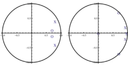
A white Gaussian signal with standard deviation 15 is used as input signal to a system with the Wiener-Ham-merstein structure. Figure 2 depicts the poles and zeros of the two linear parts and Figure 5 a) shows the nonlin-earity which is between them. The exact mathematical definition of the system is given in Appendix A.
o o x x -1.0 -0.5 0.5 1.0 -1.0 -0.5 0.5 1.0 o o o x x x -1.0 -0.5 0.5 1.0 -1.0 -0.5 0.5 1.0
Fig. 2. Poles (x) and zeros (o) of the two linear parts of the true system.
With this true system, 2000 data samples where gener-ated,{u(t), y(t)}2000
t=1 where the output is corrupted with
white Gaussian noise with standard deviation 0.1. This gives a signal-to-noise amplitude ratio of 57.
The first step of the algorithm is to estimate a linear model. In the example the search for the best linear model is skipped and the prior knowledge that it should be of 5th order is used. See any standard literature on system identification for strategies to obtain the best linear model, eg [11, 12, 19]. In Figure 3 the simulation with the 5th order linear model is shown together with the true output. The poles and zeros of the linear model
0 500 1000 1500 2000 -20 -15 -10 -5 0 5 10 15
Output signal: 1 RMSE: 1.75245
Fig. 3. Output signal (solid) together with the simulated output of the linear model (dashed).
are shown in Figure 4 a). Two zeros are clearly incor-rect compared to the true positions shown in Figure 2 but the rest of the poles and zeros seem to be reasonably well estimated.
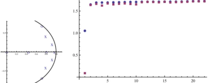
The linear model is now partitioned into two linear parts which should be at least first order systems. This gives 22 partitions and all of these are extended with a first order spline with 8 knots, ie, a local linear function with 9 segments. The positions of the knots are distributed so that each segment contains the same number of data. Given the division of the linear model and the positions of the knots, the nonlinearity can be initialized accord-ing to (12). The models are sorted accordaccord-ing to their fit at the initialization and the result is shown in Figure 4 b). The best initialization has a RMS fit of 1.05 com-pared to 1.75 for the linear model. The initialization of all 22 models took 35 CPU seconds on an average PC of the time of this paper. The bullets shows the RMS
o o o o o x x x x x 0.2 0.4 0.6 0.8 1.0 -0.5 0.5 æ æ æ æ æ ææ æ æ æ æ æ æ æ æ æ æ æ æ æ æ æ à à à à à à à à à àà à à à à à à à à à à à 5 10 15 20 0.5 1.0 1.5
Fig. 4. a) Poles (x) and zeros (o) of the linear model. b) Bullets: The RMS error of the 22 initialized Wiener-Ham-merstein models. Squares: The obtained RMS after fitting all parameters of the 22 models.
after initialization. The best initialization outperforms the other. In the same figure the fit after that all param-eters have been fitted, is also shown with squares. The best initialized model is also the one which gives the best fit after that the criterion has been minimized with re-spect to all parameters. It has an RMS fit of 0.095 which corresponds with the noise level.
In Figure 5 a) the estimated nonlinearity at initialization and for the final model are shown together with the true nonlinearity.
Since poles and zeros cannot move from one linear part to the other, it is clear that the most important issue is to have the right number of poles and zero in each one of them. For this example, out of the 22 partitions, 8 of these have the correct number of poles and zeros in each linear part. That is, all of these could converge to the best model if they would not get caught in any local minima. Figure 5 b) shows the criterion decrease for these 8 models.
-20 -10 10 20 -30 -20 -10 10 20 30 5 10 15 20 25 30 0.5 1.0 1.5 2.0 2.5 3.0
Fig. 5. a) Solid, true nonlinearity, dashed estimate at the initialization, dashed-dotted after estimating all parameters. b) Criterion decrease for the 8 initializations with correct number of zeros and poles in the linear parts. The ones with incorrect positions of poles and/or zeros either converge very slow or they are caught in bad local minima.
Clearly, the proposed initialization gives a good initial-ization so that only 10 iterations are needed in the re-cursive minimization. Some of the other initializations might lead to a good minimum if many more iterations would be applied, but after 30 iterations only a few of them have not yet terminated due to convergence to a local minimum, and their decrease is very slow.
8 Conclusions
A novel algorithm for initializing Wiener-Hammerstein models has been proposed. It starts with a best linear model which is partitioned in all possible ways into two linear sub-models. Using LS the nonlinearity between the two linear parts can efficiently be initialized. The ini-tialized models can be ranked, and the one with the best fit is the one with best chances to converge to the global minimum when all parameters are estimated simultane-ously. Consistency of the algorithm has been shown. Fi-nally the algorithm has been illustrated with an example which shows that it can really make a difference.
Acknowledgment
This work is sponsored by the Fund for Scientific Re-search (FWO-Vlaanderen), the Flemish Government (Methusalem 1), and the Belgian Federal Government (IUAP VI/4). The research was performed during Jonas Sj¨oberg’s sabbatical at Vrije Universiteit Brussel, 2009-2010.
A True Wiener-Hammerstein system
The data used in the example in Section 7 where gen-erated by the Wiener-Hammerstein system with of the following form of the two linear partsG1(q−1) = (q2−
1.4q+ 0.5)/(q2−1.6q+ 0.8) and G
2(q−1) = (0.01q3−
0.014q2+0.0098q)/(q3−2.8q2+2.6528q−0.850944). The
poles and zeros of these transfer functions are depicted in Figure 2. The nonlinearity, depicted in Figure 5 a), is formally defined as f(z) = 1.5z+ 4.5 z <−15 0.3z−13.5 −15< z <−5 3z −5< z <5 0.3z+ 13.5 5< z <15 1.5z−4.5 15< z . (A.1) References
[1] S.A. Billings and S.Y. Fakhouri. Identification of systems containing linear dynamic and static nonlinear elements.
Automatica, 18:15–26, 1982.
[2] M. Boutayeb and M. Darouach. Recursive identification
method for MISO Wiener-Hammerstein model.IEEE Trans.
Automat. Contr., 40:287–291, 1995.
[3] D.R. Brillinger. The identification of a particular nonlinear
time series system.Biometrika, 64(3):509–515, 1977.
[4] C.H. Chen and S.D. Fassois. Maximum likelihood
identification of stochastic Wiener- Hammerstein-type
nonlinear systems.Mech. Syst. Signal Process., 6(2):135–153,
1992.
[5] P. Crama and J. Schoukens. Computing an initial estimate of a Wiener-Hammerstein system with a random phase
multisine excitation. IEEE Trans. Instrum. Meas, 54:117–
122, 2005.
[6] M. Enqvist and L. Ljung. Linear approximations of nonlinear
FIR systems for separable input processes. Automatica,
41(3):459 – 473, 2005.
[7] E.W. Bai and D. Li. Convergence of the iterative
Hammerstein system identification algorithm. Automatic
Control, IEEE Transactions on, 49(11):1929 – 1940, nov. 2004.
[8] A. Juditsky, H. Hjalmarsson, A. Benveniste, B. Deylon,
L. Ljung, J. Sj¨oberg, and Q. Zhang. Nonlinear black-box
models in system identification : Mathematical foundations.
Automatica, 31(12), December 1995.
[9] L. Lauwers, R. Pintelon, and J. Schoukens. Modelling
of Wiener-Hammerstein systems via the Best Linear
Approximation. In Preprint, 15th IFAC Symposium on
System Identification Saint-Malo, France, pages 1098–1103, July 2009.
[10] L. Ljung. Convergence analysis of parametric identification
methods. IEEE Transactions on Automatic Control, 1978.
[11] L. Ljung. System Identification: Theory for the User.
Prentice-Hall, Englewood Cliffs, NJ, 2nd edition, 1999.
[12] R. Pintelon and J. Schoukens. System Identification: A
Frequency Domain Approach. IEEE-press, Piscataway, 2001. [13] J. Schoukens, T. Dobrowiecki, and R. Pintelon. Parametric and nonparametric identification of linear systems in the presence of nonlinear distortions - a frequency domain
approach. IEEE Transactions on Automatic Control,
43(2):176–190, 1998.
[14] J. Schoukens, R. Pintelon, T. Dobrowiecki, and Y. Rolain. Identification of linear systems with nonlinear distortions.
Automatica, 41:451–504, 2005.
[15] J. Schoukens, R. Pintelon, J. Paduart, and G. Vandersteen. Nonparametric initial estimates for Wiener-Hammerstein
systems. In Preprint, 14th IFAC Symposium on System
Identification, Newcastle, Australia, pages 778–783, March 2006.
[16] J. Schoukens, W.D. Widanage, K.R. Godfrey, and
R. Pintelon. Initial estimates for the dynamics of a
Hammerstein system. Automatica, 43(7):1296 – 1301, 2007.
[17] J. Sj¨oberg and H. Hjalmarsson. A system, signal,
and identification toolbox in mathematica with symbolic
capabilities. InPreprint, 15th IFAC Symposium on System
Identification Saint-Malo, France, pages 747–751, July 2009.
[18] J. Sj¨oberg, Q. Zhang, L. Ljung, A. Benveniste, B. Deylon,
P-Y. Glorennec, H. Hjalmarsson, and A. Juditsky.
Non-linear black-box modeling in system identification: a unified
overview. Automatica, 31(12):1691–1724, 1995.
[19] T. S¨oderstr¨om and P. Stoica.System Identification.
Prentice-Hall International, Hemel Hempstead, Hertfordshire, 1989.
[20] M. Verhaegen and D. Westwick. Identifying MIMO
Hammerstein systems in the context of subspace model
identification methods. Int. J. Control, 1996.
[21] J. V¨or¨os. Parameter identification of Wiener systems with
multisegment piecewise-linear nonlinearities. Systems &
Control Letters, 56(2):99 – 105, 2007.
[22] T. Wigren. Recursive prediction error identification using
the nonlinear Wiener model.Automatica, 29(4):1011 – 1025,
1993.
[23] A. Wills and B. Ninness. Estimation of generalised
Wiener-Hammerstein systems. In Preprint, 15th IFAC Symposium
on System Identification, Saint-Malo, France, pages 1104– 1109, July 2009.