37
Hard Disk Drives
The last chapter introduced the general concept of an I/O device and showed you how the OS might interact with such a beast. In this chapter, we dive into more detail about one device in particular: thehard disk drive. These drives have been the main form of persistent data storage in computer systems for decades and much of the development of file sys-tem technology (coming soon) is predicated on their behavior. Thus, it is worth understanding the details of a disk’s operation before building the file system software that manages it. Many of these details are avail-able in excellent papers by Ruemmler and Wilkes [RW92] and Anderson, Dykes, and Riedel [ADR03].
CRUX: HOWTOSTOREANDACCESSDATAONDISK
How do modern hard-disk drives store data? What is the interface? How is the data actually laid out and accessed? How does disk schedul-ing improve performance?
37.1 The Interface
Let’s start by understanding the interface to a modern disk drive. The basic interface for all modern drives is straightforward. The drive consists of a large number of sectors (512-byte blocks), each of which can be read or written. The sectors are numbered from0ton−1on a disk withn sectors. Thus, we can view the disk as an array of sectors;0ton−1is thus theaddress spaceof the drive.
Multi-sector operations are possible; indeed, many file systems will read or write 4KB at a time (or more). However, when updating the disk, the only guarantee drive manufactures make is that a single 512-byte write isatomic(i.e., it will either complete in its entirety or it won’t complete at all); thus, if an untimely power loss occurs, only a portion of a larger write may complete (sometimes called atorn write).
0 11 10 9 8 7 6 5 4 3 2 1 Spindle
Figure 37.1:A Disk With Just A Single Track
There are some assumptions most clients of disk drives make, but that are not specified directly in the interface; Schlosser and Ganger have called this the “unwritten contract” of disk drives [SG04]. Specifically, one can usually assume that accessing two blocks that are near one-another within the drive’s address space will be faster than accessing two blocks that are far apart. One can also usually assume that accessing blocks in a contiguous chunk (i.e., a sequential read or write) is the fastest access mode, and usually much faster than any more random access pattern.
37.2 Basic Geometry
Let’s start to understand some of the components of a modern disk. We start with aplatter, a circular hard surface on which data is stored persistently by inducing magnetic changes to it. A disk may have one or more platters; each platter has 2 sides, each of which is called a sur-face. These platters are usually made of some hard material (such as aluminum), and then coated with a thin magnetic layer that enables the drive to persistently store bits even when the drive is powered off.
The platters are all bound together around thespindle, which is con-nected to a motor that spins the platters around (while the drive is pow-ered on) at a constant (fixed) rate. The rate of rotation is often measured in
rotations per minute (RPM), and typical modern values are in the 7,200 RPM to 15,000 RPM range. Note that we will often be interested in the time of a single rotation, e.g., a drive that rotates at 10,000 RPM means that a single rotation takes about 6 milliseconds (6 ms).
Data is encoded on each surface in concentric circles of sectors; we call one such concentric circle atrack. A single surface contains many thou-sands and thouthou-sands of tracks, tightly packed together, with hundreds of tracks fitting into the width of a human hair.
To read and write from the surface, we need a mechanism that allows us to either sense (i.e., read) the magnetic patterns on the disk or to in-duce a change in (i.e., write) them. This process of reading and writing is accomplished by thedisk head; there is one such head per surface of the drive. The disk head is attached to a singledisk arm, which moves across the surface to position the head over the desired track.
Head Arm 0 11 10 9 8 7 6 5 4 3 2 1 Spindle Rotates this way
Figure 37.2:A Single Track Plus A Head
37.3 A Simple Disk Drive
Let’s understand how disks work by building up a model one track at a time. Assume we have a simple disk with a single track (Figure 37.1).
This track has just 12 sectors, each of which is 512 bytes in size (our typical sector size, recall) and addressed therefore by the numbers 0 through 11. The single platter we have here rotates around the spindle, to which a motor is attached. Of course, the track by itself isn’t too interesting; we want to be able to read or write those sectors, and thus we need a disk head, attached to a disk arm, as we now see (Figure 37.2).
In the figure, the disk head, attached to the end of the arm, is posi-tioned over sector 6, and the surface is rotating counter-clockwise.
Single-track Latency: The Rotational Delay
To understand how a request would be processed on our simple, one-track disk, imagine we now receive a request to read block 0. How should the disk service this request?
In our simple disk, the disk doesn’t have to do much. In particular, it must just wait for the desired sector to rotate under the disk head. This wait happens often enough in modern drives, and is an important enough component of I/O service time, that it has a special name:rotational de-lay(sometimesrotation delay, though that sounds weird). In the exam-ple, if the full rotational delay isR, the disk has to incur a rotational delay of aboutR
2 to wait for 0 to come under the read/write head (if we start at 6). A worst-case request on this single track would be to sector 5, causing nearly a full rotational delay in order to service such a request.
Multiple Tracks: Seek Time
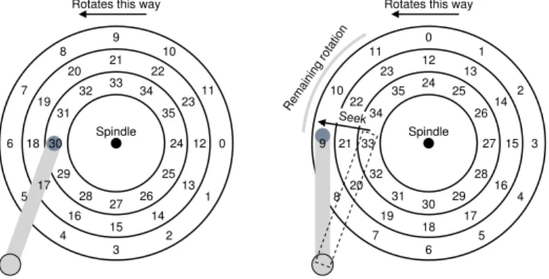
So far our disk just has a single track, which is not too realistic; modern disks of course have many millions. Let’s thus look at ever-so-slightly more realistic disk surface, this one with three tracks (Figure 37.3, left).
In the figure, the head is currently positioned over the innermost track (which contains sectors 24 through 35); the next track over contains the next set of sectors (12 through 23), and the outermost track contains the first sectors (0 through 11).
0 11 10 9 8 7 6 5 4 3 2 1 12 23 22 21 20 19 18 17 16 15 14 13 24 35 34 33 32 31 30 29 28 27 26 25 Spindle Rotates this way
Seek Remaining rotation 3 2 1 0 11 10 9 8 7 6 5 4 15 14 13 12 23 22 21 20 19 18 17 16 27 26 25 24 35 34 33 32 31 30 29 28 Spindle Rotates this way
Figure 37.3:Three Tracks Plus A Head (Right: With Seek)
To understand how the drive might access a given sector, we now trace what would happen on a request to a distant sector, e.g., a read to sector 11. To service this read, the drive has to first move the disk arm to the cor-rect track (in this case, the outermost one), in a process known as aseek. Seeks, along with rotations, are one of the most costly disk operations.
The seek, it should be noted, has many phases: first anacceleration
phase as the disk arm gets moving; thencoastingas the arm is moving at full speed, thendecelerationas the arm slows down; finallysettlingas the head is carefully positioned over the correct track. Thesettling time
is often quite significant, e.g., 0.5 to 2 ms, as the drive must be certain to find the right track (imagine if it just got close instead!).
After the seek, the disk arm has positioned the head over the right track. A depiction of the seek is found in Figure 37.3 (right).
As we can see, during the seek, the arm has been moved to the desired track, and the platter of course has rotated, in this case about 3 sectors. Thus, sector 9 is just about to pass under the disk head, and we must only endure a short rotational delay to complete the transfer.
When sector 11 passes under the disk head, the final phase of I/O will take place, known as thetransfer, where data is either read from or written to the surface. And thus, we have a complete picture of I/O time: first a seek, then waiting for the rotational delay, and finally the transfer.
Some Other Details
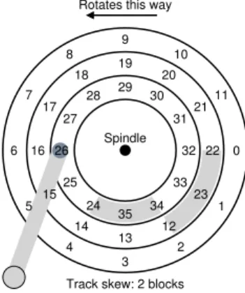
Though we won’t spend too much time on it, there are some other inter-esting details about how hard drives operate. Many drives employ some kind oftrack skewto make sure that sequential reads can be properly serviced even when crossing track boundaries. In our simple example disk, this might appear as seen in Figure 37.4.
Track skew: 2 blocks 0 11 10 9 8 7 6 5 4 3 2 1 22 21 20 19 18 17 16 15 14 13 12 23 32 31 30 29 28 27 26 25 24 35 34 33 Spindle Rotates this way
Figure 37.4:Three Tracks: Track Skew Of 2
Sectors are often skewed like this because when switching from one track to another, the disk needs time to reposition the head (even to neigh-boring tracks). Without such skew, the head would be moved to the next track but the desired next block would have already rotated under the head, and thus the drive would have to wait almost the entire rotational delay to access the next block.
Another reality is that outer tracks tend to have more sectors than inner tracks, which is a result of geometry; there is simply more room out there. These tracks are often referred to asmulti-zoneddisk drives, where the disk is organized into multiple zones, and where a zone is con-secutive set of tracks on a surface. Each zone has the same number of sectors per track, and outer zones have more sectors than inner zones.
Finally, an important part of any modern disk drive is itscache, for historical reasons sometimes called atrack buffer. This cache is just some small amount of memory (usually around 8 or 16 MB) which the drive can use to hold data read from or written to the disk. For example, when reading a sector from the disk, the drive might decide to read in all of the sectors on that track and cache them in its memory; doing so allows the drive to quickly respond to any subsequent requests to the same track.
On writes, the drive has a choice: should it acknowledge the write has completed when it has put the data in its memory, or after the write has actually been written to disk? The former is calledwrite backcaching (or sometimesimmediate reporting), and the latterwrite through. Write back caching sometimes makes the drive appear “faster”, but can be dan-gerous; if the file system or applications require that data be written to disk in a certain order for correctness, write-back caching can lead to problems (read the chapter on file-system journaling for details).
ASIDE:DIMENSIONALANALYSIS
Remember in Chemistry class, how you solved virtually every prob-lem by simply setting up the units such that they canceled out, and some-how the answers popped out as a result? That chemical magic is known by the highfalutin name ofdimensional analysisand it turns out it is useful in computer systems analysis too.
Let’s do an example to see how dimensional analysis works and why it is useful. In this case, assume you have to figure out how long, in mil-liseconds, a single rotation of a disk takes. Unfortunately, you are given only theRPMof the disk, orrotations per minute. Let’s assume we’re talking about a 10K RPM disk (i.e., it rotates 10,000 times per minute). How do we set up the dimensional analysis so that we get time per rota-tion in milliseconds?
To do so, we start by putting the desired units on the left; in this case, we wish to obtain the time (in milliseconds) per rotation, so that is ex-actly what we write down: T ime1Rotation(ms). We then write down everything
we know, making sure to cancel units where possible. First, we obtain 1minute
10,000Rotations (keeping rotation on the bottom, as that’s where it is on
the left), then transform minutes into seconds with 60seconds
1minute, and then
finally transform seconds in milliseconds with 1000ms
1second. The final result is
the following (with units nicely canceled):
T ime(ms) 1Rot. = 1✘✘minute✘ 10,000Rot.· 60✘✘seconds✘ 1✘✘minute✘ · 1000ms 1✘✘second✘= 60,000ms 10,000Rot. = 6ms Rotation
As you can see from this example, dimensional analysis makes what seems intuitive into a simple and repeatable process. Beyond the RPM calculation above, it comes in handy with I/O analysis regularly. For example, you will often be given the transfer rate of a disk, e.g., 100 MB/second, and then asked: how long does it take to transfer a 512 KB block (in milliseconds)? With dimensional analysis, it’s easy:
T ime(ms) 1Request = 512✟KB✟ 1Request · 1✟M B✟ 1024✟KB✟· 1✘✘second✘ 100✟M B✟· 1000ms 1✘✘second✘= 5ms Request
37.4 I/O Time: Doing The Math
Now that we have an abstract model of the disk, we can use a little analysis to better understand disk performance. In particular, we can now represent I/O time as the sum of three major components:
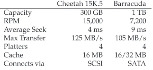
Cheetah 15K.5 Barracuda Capacity 300 GB 1 TB RPM 15,000 7,200 Average Seek 4 ms 9 ms Max Transfer 125 MB/s 105 MB/s Platters 4 4 Cache 16 MB 16/32 MB Connects via SCSI SATA
Figure 37.5:Disk Drive Specs: SCSI Versus SATA
Note that the rate of I/O (RI/O), which is often more easily used for
comparison between drives (as we will do below), is easily computed from the time. Simply divide the size of the transfer by the time it took:
RI/O=
SizeT ransf er TI/O
(37.2)
To get a better feel for I/O time, let us perform the following calcu-lation. Assume there are two workloads we are interested in. The first, known as therandomworkload, issues small (e.g., 4KB) reads to random locations on the disk. Random workloads are common in many impor-tant applications, including database management systems. The second, known as thesequentialworkload, simply reads a large number of sec-tors consecutively from the disk, without jumping around. Sequential access patterns are quite common and thus important as well.
To understand the difference in performance between random and se-quential workloads, we need to make a few assumptions about the disk drive first. Let’s look at a couple of modern disks from Seagate. The first, known as the Cheetah 15K.5 [S09b], is a high-performance SCSI drive. The second, the Barracuda [S09a], is a drive built for capacity. Details on both are found in Figure 37.5.
As you can see, the drives have quite different characteristics, and in many ways nicely summarize two important components of the disk drive market. The first is the “high performance” drive market, where drives are engineered to spin as fast as possible, deliver low seek times, and transfer data quickly. The second is the “capacity” market, where cost per byte is the most important aspect; thus, the drives are slower but pack as many bits as possible into the space available.
From these numbers, we can start to calculate how well the drives would do under our two workloads outlined above. Let’s start by looking at the random workload. Assuming each 4 KB read occurs at a random location on disk, we can calculate how long each such read would take. On the Cheetah:
TIP: USEDISKSSEQUENTIALLY
When at all possible, transfer data to and from disks in a sequential man-ner. If sequential is not possible, at least think about transferring data in large chunks: the bigger, the better. If I/O is done in little random pieces, I/O performance will suffer dramatically. Also, users will suffer. Also, you will suffer, knowing what suffering you have wrought with your careless random I/Os.
The average seek time (4 milliseconds) is just taken as the average time reported by the manufacturer; note that a full seek (from one end of the surface to the other) would likely take two or three times longer. The average rotational delay is calculated from the RPM directly. 15000 RPM is equal to 250 RPS (rotations per second); thus, each rotation takes 4 ms. On average, the disk will encounter a half rotation and thus 2 ms is the average time. Finally, the transfer time is just the size of the transfer over the peak transfer rate; here it is vanishingly small (30microseconds; note that we need 1000 microseconds just to get 1 millisecond!).
Thus, from our equation above,TI/Ofor the Cheetah roughly equals
6 ms. To compute the rate of I/O, we just divide the size of the transfer by the average time, and thus arrive atRI/Ofor the Cheetah under the
random workload of about0.66MB/s. The same calculation for the Bar-racuda yields aTI/Oof about 13.2 ms, more than twice as slow, and thus
a rate of about0.31MB/s.
Now let’s look at the sequential workload. Here we can assume there is a single seek and rotation before a very long transfer. For simplicity, assume the size of the transfer is 100 MB. Thus,TI/Ofor the Barracuda
and Cheetah is about 800 ms and 950 ms, respectively. The rates of I/O are thus very nearly the peak transfer rates of 125 MB/s and 105 MB/s, respectively. Figure 37.6 summarizes these numbers.
The figure shows us a number of important things. First, and most importantly, there is a huge gap in drive performance between random and sequential workloads, almost a factor of 200 or so for the Cheetah and more than a factor 300 difference for the Barracuda. And thus we arrive at the most obvious design tip in the history of computing.
A second, more subtle point: there is a large difference in performance between high-end “performance” drives and low-end “capacity” drives. For this reason (and others), people are often willing to pay top dollar for the former while trying to get the latter as cheaply as possible.
Cheetah Barracuda
RI/ORandom 0.66 MB/s 0.31 MB/s RI/OSequential 125 MB/s 105 MB/s
ASIDE: COMPUTINGTHE“AVERAGE” SEEK
In many books and papers, you will see average disk-seek time cited as being roughly one-third of the full seek time. Where does this come from?
Turns out it arises from a simple calculation based on average seek
distance, not time. Imagine the disk as a set of tracks, from0toN. The seek distance between any two tracksxandyis thus computed as the absolute value of the difference between them:|x−y|.
To compute the average seek distance, all you need to do is to first add up all possible seek distances:
N X x=0 N X y=0 |x−y|. (37.4)
Then, divide this by the number of different possible seeks: N2. To compute the sum, we’ll just use the integral form:
Z N
x=0
Z N
y=0
|x−y|dydx. (37.5) To compute the inner integral, let’s break out the absolute value:
Z x y=0 (x−y) dy+ Z N y=x (y−x) dy. (37.6) Solving this leads to (xy−1
2y 2) x 0+ ( 1 2y 2−xy) N
x which can be
sim-plified to(x2−N x+1 2N
2).Now we have to compute the outer integral:
Z N x=0 (x2−N x+1 2N 2) dx, (37.7) which results in:
(1 3x 3−N 2x 2+N2 2 x) N 0 = N 3 3 . (37.8)
Remember that we still have to divide by the total number of seeks (N2) to compute the average seek distance:(N3
3 )/(N 2) = 1
3N. Thus the average seek distance on a disk, over all possible seeks, is one-third the full distance. And now when you hear that an average seek is one-third of a full seek, you’ll know where it came from.
0 11 10 9 8 7 6 5 4 3 2 1 12 23 22 21 20 19 18 17 16 15 14 13 24 35 34 33 32 31 30 29 28 27 26 25 Spindle Rotates this way
Figure 37.7:SSTF: Scheduling Requests 21 And 2
37.5 Disk Scheduling
Because of the high cost of I/O, the OS has historically played a role in deciding the order of I/Os issued to the disk. More specifically, given a set of I/O requests, thedisk schedulerexamines the requests and decides which one to schedule next [SCO90, JW91].
Unlike job scheduling, where the length of each job is usually un-known, with disk scheduling, we can make a good guess at how long a “job” (i.e., disk request) will take. By estimating the seek and possi-ble rotational delay of a request, the disk scheduler can know how long each request will take, and thus (greedily) pick the one that will take the least time to service first. Thus, the disk scheduler will try to follow the
principle of SJF (shortest job first)in its operation.
SSTF: Shortest Seek Time First
One early disk scheduling approach is known asshortest-seek-time-first
(SSTF) (also calledshortest-seek-firstorSSF). SSTF orders the queue of I/O requests by track, picking requests on the nearest track to complete first. For example, assuming the current position of the head is over the inner track, and we have requests for sectors 21 (middle track) and 2 (outer track), we would then issue the request to 21 first, wait for it to complete, and then issue the request to 2 (Figure 37.7).
SSTF works well in this example, seeking to the middle track first and then the outer track. However, SSTF is not a panacea, for the following reasons. First, the drive geometry is not available to the host OS; rather, it sees an array of blocks. Fortunately, this problem is rather easily fixed. Instead of SSTF, an OS can simply implementnearest-block-first(NBF), which schedules the request with the nearest block address next.
The second problem is more fundamental: starvation. Imagine in our example above if there were a steady stream of requests to the in-ner track, where the head currently is positioned. Requests to any other tracks would then be ignored completely by a pure SSTF approach. And thus the crux of the problem:
CRUX: HOWTOHANDLEDISKSTARVATION
How can we implement SSTF-like scheduling but avoid starvation?
Elevator (a.k.a. SCAN or C-SCAN)
The answer to this query was developed some time ago (see [CKR72] for example), and is relatively straightforward. The algorithm, originally calledSCAN, simply moves back and forth across the disk servicing re-quests in order across the tracks. Let’s call a single pass across the disk (from outer to inner tracks, or inner to outer) asweep. Thus, if a request comes for a block on a track that has already been serviced on this sweep of the disk, it is not handled immediately, but rather queued until the next sweep (in the other direction).
SCAN has a number of variants, all of which do about the same thing. For example, Coffman et al. introducedF-SCAN, which freezes the queue to be serviced when it is doing a sweep [CKR72]; this action places re-quests that come in during the sweep into a queue to be serviced later. Doing so avoids starvation of far-away requests, by delaying the servic-ing of late-arrivservic-ing (but nearer by) requests.
C-SCANis another common variant, short forCircular SCAN.
In-stead of sweeping in both directions across the disk, the algorithm only sweeps from outer-to-inner, and then resets at the outer track to begin again. Doing so is a bit more fair to inner and outer tracks, as pure back-and-forth SCAN favors the middle tracks, i.e., after servicing the outer track, SCAN passes through the middle twice before coming back to the outer track again.
For reasons that should now be clear, the SCAN algorithm (and its cousins) is sometimes referred to as theelevator algorithm, because it behaves like an elevator which is either going up or down and not just servicing requests to floors based on which floor is closer. Imagine how annoying it would be if you were going down from floor 10 to 1, and somebody got on at 3 and pressed 4, and the elevator went up to 4 be-cause it was “closer” than 1! As you can see, the elevator algorithm, when used in real life, prevents fights from taking place on elevators. In disks, it just prevents starvation.
Unfortunately, SCAN and its cousins do not represent the best schedul-ing technology. In particular, SCAN (or SSTF even) do not actually adhere as closely to the principle of SJF as they could. In particular, they ignore rotation. And thus, another crux:
CRUX: HOWTOACCOUNTFORDISKROTATIONCOSTS How can we implement an algorithm that more closely approximates SJF by takingbothseek and rotation into account?
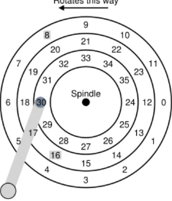
0 11 10 9 8 7 6 5 4 3 2 1 12 23 22 21 20 19 18 17 16 15 14 13 24 35 34 33 32 31 30 29 28 27 26 25 Spindle Rotates this way
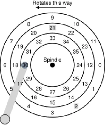
Figure 37.8:SSTF: Sometimes Not Good Enough SPTF: Shortest Positioning Time First
Before discussingshortest positioning time firstorSPTFscheduling (some-times also calledshortest access time firstorSATF), which is the solution to our problem, let us make sure we understand the problem in more de-tail. Figure 37.8 presents an example.
In the example, the head is currently positioned over sector 30 on the inner track. The scheduler thus has to decide: should it schedule sector 16 (on the middle track) or sector 8 (on the outer track) for its next request. So which should it service next?
The answer, of course, is “it depends”. In engineering, it turns out “it depends” is almost always the answer, reflecting that trade-offs are part of the life of the engineer; such maxims are also good in a pinch, e.g., when you don’t know an answer to your boss’s question, you might want to try this gem. However, it is almost always better to knowwhyit depends, which is what we discuss here.
What it depends on here is the relative time of seeking as compared to rotation. If, in our example, seek time is much higher than rotational delay, then SSTF (and variants) are just fine. However, imagine if seek is quite a bit faster than rotation. Then, in our example, it would make more sense to seekfurtherto service request 8 on the outer track than it would to perform the shorter seek to the middle track to service 16, which has to rotate all the way around before passing under the disk head.
TIP: ITALWAYSDEPENDS(LIVNY’SLAW)
Almost any question can be answered with “it depends”, as our colleague Miron Livny always says. However, use with caution, as if you answer too many questions this way, people will stop asking you questions alto-gether. For example, somebody asks: “want to go to lunch?” You reply: “it depends, areyoucoming along?”
equivalent (depending, of course, on the exact requests), and thus SPTF is useful and improves performance. However, it is even more difficult to implement in an OS, which generally does not have a good idea where track boundaries are or where the disk head currently is (in a rotational sense). Thus, SPTF is usually performed inside a drive, described below.
Other Scheduling Issues
There are many other issues we do not discuss in this brief description of basic disk operation, scheduling, and related topics. One such is-sue is this: whereis disk scheduling performed on modern systems? In older systems, the operating system did all the scheduling; after looking through the set of pending requests, the OS would pick the best one, and issue it to the disk. When that request completed, the next one would be chosen, and so forth. Disks were simpler then, and so was life.
In modern systems, disks can accommodate multiple outstanding re-quests, and have sophisticated internal schedulers themselves (which can implement SPTF accurately; inside the disk controller, all relevant details are available, including exact head position). Thus, the OS scheduler usu-ally picks what it thinks the best few requests are (say 16) and issues them all to disk; the disk then uses its internal knowledge of head position and detailed track layout information to service said requests in the best pos-sible (SPTF) order.
Another important related task performed by disk schedulers isI/O merging. For example, imagine a series of requests to read blocks 33, then 8, then 34, as in Figure 37.8. In this case, the scheduler shouldmerge
the requests for blocks 33 and 34 into a single two-block request; any re-ordering that the scheduler does is performed upon the merged requests. Merging is particularly important at the OS level, as it reduces the num-ber of requests sent to the disk and thus lowers overheads.
One final problem that modern schedulers address is this: how long should the system wait before issuing an I/O to disk? One might naively think that the disk, once it has even a single I/O, should immediately issue the request to the drive; this approach is calledwork-conserving, as the disk will never be idle if there are requests to serve. However, research onanticipatory disk schedulinghas shown that sometimes it is better to wait for a bit [ID01], in what is called anon-work-conservingapproach.
By waiting, a new and “better” request may arrive at the disk, and thus overall efficiency is increased. Of course, deciding when to wait, and for how long, can be tricky; see the research paper for details, or check out the Linux kernel implementation to see how such ideas are transitioned into practice (if you are the ambitious sort).
37.6 Summary
We have presented a summary of how disks work. The summary is actually a detailed functional model; it does not describe the amazing physics, electronics, and material science that goes into actual drive de-sign. For those interested in even more details of that nature, we suggest a different major (or perhaps minor); for those that are happy with this model, good! We can now proceed to using the model to build more in-teresting systems on top of these incredible devices.
References
[ADR03] “More Than an Interface: SCSI vs. ATA” Dave Anderson, Jim Dykes, Erik Riedel FAST ’03, 2003
One of the best recent-ish references on how modern disk drives really work; a must read for anyone interested in knowing more.
[CKR72] “Analysis of Scanning Policies for Reducing Disk Seek Times” E.G. Coffman, L.A. Klimko, B. Ryan
SIAM Journal of Computing, September 1972, Vol 1. No 3.
Some of the early work in the field of disk scheduling.
[ID01] “Anticipatory Scheduling: A Disk-scheduling Framework To Overcome Deceptive Idleness In Synchronous I/O” Sitaram Iyer, Peter Druschel
SOSP ’01, October 2001
A cool paper showing how waiting can improve disk scheduling: better requests may be on their way!
[JW91] “Disk Scheduling Algorithms Based On Rotational Position” D. Jacobson, J. Wilkes
Technical Report HPL-CSP-91-7rev1, Hewlett-Packard (February 1991)
A more modern take on disk scheduling. It remains a technical report (and not a published paper) because the authors were scooped by Seltzer et al. [SCO90].
[RW92] “An Introduction to Disk Drive Modeling” C. Ruemmler, J. Wilkes
IEEE Computer, 27:3, pp. 17-28, March 1994
A terrific introduction to the basics of disk operation. Some pieces are out of date, but most of the basics remain.
[SCO90] “Disk Scheduling Revisited” Margo Seltzer, Peter Chen, John Ousterhout USENIX 1990
A paper that talks about how rotation matters too in the world of disk scheduling.
[SG04] “MEMS-based storage devices and standard disk interfaces: A square peg in a round hole?”
Steven W. Schlosser, Gregory R. Ganger FAST ’04, pp. 87-100, 2004
While the MEMS aspect of this paper hasn’t yet made an impact, the discussion of the contract between file systems and disks is wonderful and a lasting contribution.
[S09a] “Barracuda ES.2 data sheet”
http://www.seagate.com/docs/pdf/datasheet/disc/ds cheetah 15k 5.pdfA data sheet; read at your own risk. Risk of what? Boredom.
[S09b] “Cheetah 15K.5”
http://www.seagate.com/docs/pdf/datasheet/disc/ds barracuda es.pdfSee above commentary on data sheets.
Homework
This homework usesdisk.pyto familiarize you with how a modern hard drive works. It has a lot of different options, and unlike most of the other simulations, has a graphical animator to show you exactly what happens when the disk is in action. See the README for details.
1. Compute the seek, rotation, and transfer times for the following sets of requests: -a 0,-a 6,-a 30,-a 7,30,8, and finally-a 10,11,12,13.
2. Do the same requests above, but change the seek rate to different values: -S 2,-S 4,-S 8,-S 10,-S 40,-S 0.1. How do the times change?
3. Do the same requests above, but change the rotation rate:-R 0.1,
-R 0.5,-R 0.01. How do the times change?
4. You might have noticed that some request streams would be bet-ter served with a policy betbet-ter than FIFO. For example, with the request stream-a 7,30,8, what order should the requests be pro-cessed in? Now run the shortest seek-time first (SSTF) scheduler (-p SSTF) on the same workload; how long should it take (seek,
rotation, transfer) for each request to be served?
5. Now do the same thing, but using the shortest access-time first (SATF) scheduler (-p SATF). Does it make any difference for the set of requests as specified by-a 7,30,8? Find a set of requests where SATF does noticeably better than SSTF; what are the condi-tions for a noticeable difference to arise?
6. You might have noticed that the request stream-a 10,11,12,13
wasn’t particularly well handled by the disk. Why is that? Can you introduce a track skew to address this problem (-o skew, where
skewis a non-negative integer)? Given the default seek rate, what should the skew be to minimize the total time for this set of re-quests? What about for different seek rates (e.g.,-S 2,-S 4)? In general, could you write a formula to figure out the skew, given the seek rate and sector layout information?
7. Multi-zone disks pack more sectors into the outer tracks. To config-ure this disk in such a way, run with the-zflag. Specifically, try running some requests against a disk run with-z 10,20,30(the
numbers specify the angular space occupied by a sector, per track; in this example, the outer track will be packed with a sector every 10 degrees, the middle track every 20 degrees, and the inner track with a sector every 30 degrees). Run some random requests (e.g.,
-a -1 -A 5,-1,0, which specifies that random requests should be used via the-a -1flag and that five requests ranging from 0 to the max be generated), and see if you can compute the seek, rota-tion, and transfer times. Use different random seeds (-s 1,-s 2, etc.). What is the bandwidth (in sectors per unit time) on the outer, middle, and inner tracks?
8. Scheduling windows determine how many sector requests a disk can examine at once in order to determine which sector to serve next. Generate some random workloads of a lot of requests (e.g.,
-A 1000,-1,0, with different seeds perhaps) and see how long the SATF scheduler takes when the scheduling window is changed from 1 up to the number of requests (e.g.,-w 1up to-w 1000, and some values in between). How big of scheduling window is needed to approach the best possible performance? Make a graph and see. Hint: use the-cflag and don’t turn on graphics with-G
to run these more quickly. When the scheduling window is set to 1, does it matter which policy you are using?
9. Avoiding starvation is important in a scheduler. Can you think of a series of requests such that a particular sector is delayed for a very long time given a policy such as SATF? Given that sequence, how does it perform if you use abounded SATForBSATFscheduling approach? In this approach, you specify the scheduling window (e.g.,-w 4) as well as the BSATF policy (-p BSATF); the scheduler then will only move onto the next window of requests whenallof the requests in the current window have been serviced. Does this solve the starvation problem? How does it perform, as compared to SATF? In general, how should a disk make this trade-off between performance and starvation avoidance?
10. All the scheduling policies we have looked at thus far aregreedy, in that they simply pick the next best option instead of looking for the optimal schedule over a set of requests. Can you find a set of requests in which this greedy approach is not optimal?