Validation of Spatial Prediction Models for
Landslide Hazard Mapping
CHANG-JO F. CHUNG1and ANDREA G. FABBRI2
1Geological Survey of Canada, 601 Booth Street, Ottawa, Canada K1A 0E8
(Fax: +1-613-996-3726; E-mail: [email protected]);2International Institute of Aerospace Surveying and Earth Sciences, The Netherlands (Fax: +31-53-487-4336; E-mail: [email protected])
(Received: 12 June 2001; accepted 22 May 2002)
Abstract. This contribution discusses the problem of providing measures of significance of pre-diction results when the prepre-dictions were generated from spatial databases for landslide hazard mapping. The spatial databases usually contain map information on lithologic units, land-cover units, topographic elevation and derived attributes (slope, aspect, etc.) and the distribution in space and in time of clearly identified mass movements. In prediction modelling we transform the multi-layered database into an aggregation of functional values to obtain an index of propensity of the land to failure. Assuming then that the information in the database is sufficiently representative of the typical conditions in which the mass movements originated in space and in time, the problem then, is to confirm the validity of the results of some models over other ones, or of particular experiments that seem to use more significant data. A core point of measuring the significance of a prediction is that it allows interpreting the results. Without a validation no interpretation is possible, no support of the method or of the input information can be provided. In particular with validation, the added value can be assessed of a prediction either in a fixed time interval, or in an open-ended time or within the confined space of a study area. Validation must be of guidance in data collection and field practice for landslide hazard mapping.
Key words:Validation, spatial data, prediction models, future landslide hazard, quantitative models, visualization, ranking, interpretation of prediction results
1. Introduction
This contribution deals with the issue of generating predictions from spatial data-bases for landslide hazard mapping. In particular, it discusses the problem of providing measure of significance of prediction results. For instance, if we consider a spatial database containing maps of lithologic units, of land cover units, of topo-graphic elevation and derived attributes (slope, aspect, etc.) and of the distribution in space and in time of clearly identified mass movements, we can transform the multi-layered database into an aggregation of functional] values to obtain an index of propensity of the land to failure (Chunget al., 1995, Carraraet al., 1995, Leroi, 1996, Chung and Fabbri, 1998, 1999, Jibsonet al., 1998). Assuming then that the information in the database is sufficiently representative of the typical conditions in which the mass movements originated (in space and in time), we can generate
many numerical expressions of such a property using different mathematical model and input variations. The problem then, is to confirm the validity of the results of some models over other ones, or of particular experiments that seem to use more significant data.
Such confirmation is not only to convince us of the degree of success in predict-ing, but also to communicate to non-specialists the significance of the predictions so that decisions can be taken about safer land uses as a consequence of the pre-diction results. The issue of validation is broader than landslide hazard mapping and it permeates the entire field of spatial data analysis. We will first cover the terminology to isolate basic concepts of prediction modelling, the comparisons between traditional and more quantitative models of hazard representation, the ranking order for visualization of prediction results, several validation strategies, and the prediction-rate curves in support of prediction interpretation. Two applic-ation examples describe the strategy used in this research and provide a basis for generalizing the approach to validation.
2. Definition and Terminology
Consider the construction of a landslide hazard map to identify the areas likely to be affected by future landslides. Thetarget patternis then defined as the spatial distribution of the areas to be affected by future landslides. Thestudyarea is defined as the area where we wish to have information on the target pattern. Of course, it is impossible to obtain the unknown locations of future events, future landslides that have not yet occurred. The target pattern is an unobservable and binary spatial pattern. Although we may know the characteristics and locations of past landslides in the study area, they are NOT part of the target pattern under the definition.
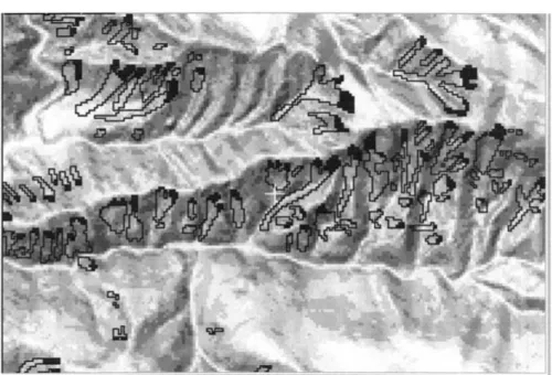
Another important consideration of defining the target pattern is illustrated by using future landslides of debris flow type. Suppose that we define as the target pattern the whole area to be affected by future debris flows. The target pattern consists of at least two separate and distinct sub-areas, the scarp area and the deposit area. We assume that the scarp identifies where the landslide starts and that the deposit area indicates where the landslide ends. The geomorphologic char-acteristics of these two sub-areas are distinctly different. Hence, it is necessary to definethe set of the scarps of all the future landslides as the new target pattern ratherthan set of the entire scars of the landslides. Without such redefinition of the target pattern, the prediction problem may not be solvable. In Figure 1, the landslides induced by the 1994 Northridge Earthquake in California were systemat-ically divided into the scarps and the remaining areas by Chung and Jibson (2002). The resulting prediction pattern should now identify the locations of the scarps of future landslides from the information about the scarps of the past landslides. After identification of the scarps of possible future landslides, simulations with cellular automata (Packard and Wolfram, 1985) or similar techniques can be employed, for example, to generate possible deposit areas of the future landslides.
Figure 1. Scars of the past landslides induced by the 1994 Northridge Earthquake in Califor-nia, U.S.A. The areas shown in black within the landslide bodies were considered as scarps of the landslides.
While the target patterns are the unknown that we wish to have,the prediction imagesare what we can generate for the target patterns using prediction models.
The prediction modelsare defined as logical or analytical procedures to construct
prediction imagesfor given target patterns. They range from simple ad-hoc proced-ures, to complex mathematical or statistical analyses, and to models based on an expert’s qualitative knowledge. We attempt to generate prediction images, which “approximate” as closely as possible the unknown and unobservable target pat-terns. We define aprediction patternas a thematic representation of the prediction image to visualize and perceive it.
3. Traditional Models
Traditionally a geomorphologist, who is an expert on earth surface processes, con-structs a landslide hazard map for identifying areas likely to be affected by future landslides (i.e.,a prediction pattern). This is to guide the decision makers for land-use planning in the study area. From a limited number of field observations, the scientist will produce a geomorphologic map showing the basic characteristics of landforms. From that the expert has to identify typical situations (such as combina-tions of landforms) that characterize the level of hazard as low, medium or high. A qualitative hazard mapping north of Lisbon, in Portugal, was discussed by Zêzere (1996a). It is an application based on a systematic inventory of mass movements in the same region (Zêzere, 1996b). In that study, the number of past landslides
in each landform unit simply determined the level of hazard. Panizzaet al.(1998) proposed a new legend for geomorphologic maps applied to hazard levels. In their legend a separation was made between landforms, processes and deposits. Based on the new legend, it seems possible to systematically produce hazard maps. Haz-ard levels were constructed by classifying the observed landforms into gravitational deposits and eroded features. Hence, it is difficult to assign quantitative scores or values to these qualitative hazard levels.
Mathematically oriented geomorphologists and civil engineers have been trying to construct deterministic models for slope stability by studying and interpreting the physical processes of mass movements using variables such as slope angle, soil cohesion, water saturation capacity, and shearing resistance. Using the models, they have generated safety factor maps for slope failure (Terlienet al., 1995) and the safety factor maps are used to represent the prediction patterns for future land-slide hazard. While the hazard maps derived from geomorphologic maps usually consisted of three to five levels of hazard, the safety factor maps can be shown in a continuous scale.
To represent the predictions, Varnes (1984) introduced the term landslide hazard “zonation” as a quantitative measure of landslide hazard (Varnes, 1984; Carraraet al., 1995). Examples of geomorphologic maps and of the corresponding hazard zonation maps can be found in Varnes (1984). Van Westen (1993) also discussed the need to separate the basic themes from geomorphologic maps to represent in a systematic manner the distribution of all the geomorphologic factors used in hazard zonation. To produce a map showing landslide hazard zonation, the geo-morphologic synthesis by experts should be a consistent and logical process. As the number of landforms and other spatial information to be considered increases, it is harder, if not impossible, to achievedata consistency. Though a geomorphologic map containing the basic landforms emphasizes the geomorphologic processes, it cannot include all related pieces of information such as slope, aspect and vegetation even though they are used in its construction. However, if the related information is significant to the hazard map, then it must be directly considered in a quantitative evaluation of hazard and in the corresponding hazard levels to represent.
With respect to future landslide hazard, regardless of how the hazard prediction maps were generated using the traditional models, the two main weaknesses of the hazard maps by experts (either geomorphologists or civil engineers) are: (1) the in-terpretation of the hazard levels of the maps; and (2) the “independent” verification of the hazard maps. For example, suppose that a road is planned to go through a “high hazard” area of a map based on a geomorphologic study. What does “high hazard” mean? Can we link this “high” to the probability that a future landslide will affect the intersecting portion of the road within the next 50 years? Without estimating such a probability, the decision makers cannot perform an adequate economic cost-benefit analysis to make the proper land-use planning. A similar argument can be made for the safety factor map for slope failure. As we will see, the most important question for the hazard maps is “how good are the prediction
results with respect to the future landslide hazard?” Obviously, it is not clear yet how we can verify the prediction in the maps.
4. Quantitative Models
For the past two decades, several quantitative spatial prediction models for identi-fying hazardous areas to be affected by future landslides have also been developed (Wang and Unwin, 1992; Chunget al., 1995; Carraraet al., 1995; Chung and Fab-bri, 1998, 1999; Jibsonet al., 1998). In these quantitative models, the hazard levels of the prediction results were expressed in terms of mathematical functions such as probability functions in a continuous scale. When the probability function is used to express the hazard of future landslides, it appears that the numeric representations can be interpreted as quantitative measures of the hazard. For example a pixel in a quantitative hazard map generated using a probability function is assigned a value of 60%. It may then be interpreted as “the estimated probability that the pixel will be affected by a future landslide is 60%”. Although such an explicit statement is desirable for a prediction map, the question is: “What assumptions are required to make such a statement reasonable?”
Let us review the sentence “the estimated probability that the pixel will be affected by a future landslide is 60%”. At a first glance, the sentence appears reasonable, but it is insignificant without “future landslide” being connected to a time period such as the next 30 years or the next 100,000,000 years. Without such a time period, the statement is meaningless. If the 60% probability is for landslides occurring during the next 30 years, then obviously we must avoid the area for any future development. However if the probability is for the next 100 million years, then we shouldn’t take the prediction so seriously.
The next question is: “What assumptions were made to estimate the 60% prob-ability within the next 30 years?” In estimating the probprob-ability, an assumption that there would be 7 future landslides in the study area would be significantly different from an assumption that there would be 1,000 landslides in the area within the next 30 years. Similarly, the assumptions on the sizes of the future landslides play a significant role in estimating probability. Without such assumptions on the number (or its distribution) and the size distribution of future landslides, the estimation of the probability is not possible. However, if the assumptions were extremely rigid and/or too unrealistic, then the estimated probability would again be worthless.
Let us consider a prediction classR of the size ofr km2in a prediction pattern
for a study area,T of the size oft km2. To study the unknown probability that a
future landslide within the next 30 years will affect a pixel within this prediction class, we must assume two values: (i) the target area, Ato be affected by future landslides isα km2, and (ii) the portion of future landslides of α km2 that has occurred within that class isq.
For a given prediction class, the probability that a pixel within the class will affected by a future landslide is then obtained byq/r. This probability should be
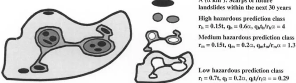
Figure 2. The study area,T of the size of t km2, includes three prediction classes, high, medium and low of a prediction pattern and the target area. We assume that the target pattern, A to be affected by future landslides isαkm2, the scarps of future landslides are known. Both the high and medium prediction classes occupy 15% each of the study area but they predict 60% and 20% respectively of future landslides and the scarps of future landslides occupies 10% of the study area:rh=0.15t,qh=0.6α,rm=0.15t,qm=0.2α,rl=0.7t,ql =0.2α andα=0.1t. Thereforeqhth/rhα=4,qmtm/rmα=1.33 andqltl/rlα=0.29.
compared with the probability of any pixel in the study area to be affected by a future landslide, α/t. It is the same probability for a pixel in a prediction class consisting of a random collection of pixels. To look at the “predictive power” of a prediction class, the ratio:
qt
rα, (1)
ofq/randα/tprovides a measurement for the corresponding class and it is termed “ratio of effectiveness” for the corresponding prediction class. If the ratio for a prediction class is near 1, then it implies that the class consists of randomly selected pixels and hence is an unsupportive prediction class. To make a “powerful and ef-fective” prediction class, the ratio should be either very large or near zero regardless of the type of the prediction model used to obtain a prediction pattern. From our experience, the ratio of effectiveness should be either larger than at least 3 or less than at most 0.2 for a prediction class to be significant. To indicate significantly effective classes, the ratios are preferably larger than 6 or less than 0.1.
To illustrate the idea, Figure 2 includes three prediction classes, high, medium and low of a prediction pattern and the target area in a study area. We assume that the target pattern, the scarps of future landslides are known. Both the high and medium prediction classes occupy 15% each of the study area but they predict 60% and 20% respectively of future landslides and the scarps of future landslides occupies 10% of the study area:rh = 0.15t,qh = 0.6α,rm = 0.15t,qm = 0.2α, rl = 0.7t, ql = 0.2α andα = 0.1t. Thereforeqhth/rhα = 4, qmtm/rmα = 1.33 and qltl/rlα = 0.29. It implies that the medium and low classes don’t provide effective prediction power. However, the high class provides reasonably effective hazard area.
A very important point is that the probabilities cannot be discussed without two assumptions on the size of the future landslides,αand their proportion in the class,
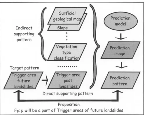
Figure 3. The construction of a prediction map for future landslide hazard. The diagram provides an example of the proposition and related symbolic relationships among the target pattern, direct supporting pattern, indirect supporting patterns, and prediction model, image and patterns.
q. Obviously, in real life, we do not have these two values. Through the validation procedure discussed later, we will propose a method for realistically assessing these values in real situations.
Our approach stems from the same needs to generate thematic maps based on the same spatial data used by the experts. We refer our approach to the prediction model as the “favorability function” approach (Chung and Fabbri, 1993), illustrated in Figure 3. The favorability function approach requires the two assumptions that: (i) the target pattern can be characterized by the geomorphologic spatial data, and (ii) the events related to the target pattern will occur in the future under similar geomorphologic circumstances.
However, we introduce here not only quantitative models and systematic spatial data analysis, but also the “independent” validation of the prediction results with respect to future landslides. Additionally, but most significantly, using the cross-validation procedure, we illustrate how to estimate the probability that a pixel will be affected by a future landslide within the next 35 years using La Baie study area in the Canadian Province of Quebéc. Through this procedure, we will also provide the exact assumptions that we make in estimating the probability.
5. Visualization
When a landslide hazard map consists of three to five levels of hazard, it is trivial to visualize such thematic representation on a computer monitor or on a printer. However, the situation changes if a prediction image for a landslide hazard is constructed using a mathematical prediction model by computing a predicted value at each pixel in a continuous scale. In this case, by slicing the predicted pixel value in the prediction image, a prediction pattern is obtained, and it can be subsequently visualized and interpreted. How to slice it is not a trivial matter: it becomes the next important step in modelling.
There are two ways of making the prediction classes (each class represents one level of hazard) for a prediction pattern from the pixel values. (1)Equal-interval classes. The range of all the pixel values is divided into a number of equal intervals. The ranges of the intervals are identical and one class is assigned to each interval. At each interval, the pixels whose values lie within the interval are assigned to the class. The numbers of pixels in the classes are very different. (2) Ranking equal-numberclasses. All pixels are sorted according the pixel value in descending order. The total number of pixels is divided into a number of classes with equal number of pixels. The first class consists of the pixels with the largest pixel values and the next subsequent class is made up of the pixels with the next largest values. Each class consists of the equal number of pixels (Chung and Fabbri, 1999).
Very frequently, the number of classes can be represented by an 8-bit value ranging from 0 to 255. By assigning a color for each 8-bit value, a “pseudo-color look-up table” is constructed. Using the look-up table, the 8-bit prediction pattern is then visualized on a computer screen or a printer.
Suppose that we have obtained two prediction images from two different pre-diction models, and we wish to compare these two images. The pixel values from two prediction images may have two different meanings. For instance, while the predicted values in a probability model (Chung and Fabbri, 1999) represent the probability values, the pixel values in a fuzzy set model (Chung and Fabbri, 2001) are the membership function scores. In this instance, the two pixel values are not compatible. For an objective and proper comparison of the prediction images, we must first obtain the two corresponding prediction patterns, which are compatible. If the prediction patterns are obtained from theequal-interval classes in way (1) above, then the comparison becomes very difficult because the two patterns may not be compatible except for some special cases. However, if we obtain the two prediction patterns using theranking equal-numberclasses in way (2) above, then their comparison becomes a trivial matter. That is, the numbers of pixels in the first class (with the highest values) of the two prediction patterns are the same and the sizes of the two first classes are the same. These twoclassesalso represent the most hazardous areas for future landslides regardless of the models. If we expect fewer future landslides in one of these first classes than in the other, then we could
conclude that the model with the first class with more landslides provides a better prediction.
Consider two predicted values of two pixels in the prediction image. Because both of the predicted values in the prediction image are subjected to the same assumptions, the relative hazard from the predicted values can be maintained (even if there may be a problem with the assumptions). It implies that the ranking of the predicted pixel values in the image is more significant than the original predicted values. It is one of many reasons why we prefer to use the second ranking equal number classes to generate a prediction pattern. We will exploit the ranking to obtain a prediction pattern.
6. Ranking Procedure
In the second ranking equal number classes for slicing to obtain a prediction pattern from a prediction image, instead of the original predicted value at each pixel, we use the ranking of the predicted value. Suppose that we have 1,000,000 pixels in a study area. From an image, we have obtained 1,000,000 predicted values, one at each pixel. We sort all of the 1,000,000 values in decreasing order. Then for each pixel, we replace the predicted value by the corresponding rank divided by the number of pixels in the entire study area, i.e., 1,000,000. The revised value of the pixel with the largest predicted value, the most hazardous predicted pixel, has the value 1, and the pixel with the smallest pixel value has value of 0.000001 (= 1/1,000,000). We define it as a “ranking” process in modelling and the revised values ranging between 0 and 1 are termed “ranks”. After the ranking, by slicing these revised values between 0 and 1, we obtain a prediction pattern.
At each pixel, we have two values, the original predicted value and the corres-ponding rank. To look at the relationship, we can make a scatter plot of these pairs, one point in the scatter plot for each pixel. Suppose that we assign the ranks to thex-axis and the original predicted values to the y-axis in the scatter plot. Then the dots will form a monotone non-decreasing plot. From this plot, we always obtain the exact relationships between the ranks and the original values. Figure 4 illustrates the relationship in the prediction image for Figure 6a.
Suppose that the study area consists of 400 km2 with 1,000,000 pixels with
20 m×20 m resolution. Suppose that it is economically and socially reasonable to delineate 4 km2 as being vulnerable to landslide hazards, 4 km2 which will be sterilized and effectively lose all their economic value. Therefore, from the exist-ing geoscience spatial data, we should identify the most hazardous 4 km2 areas. Regardless of the prediction model used, we should assign the 10,000 pixels with the highest predicted values to the hazardous area. Using the ranking, the selection of the 10,000 pixels becomes a trivial task.
Figure 4. Relationships between the rank order of predicted value pixels in the image of Fig-ure 6a, and the log10 of the predicted values that were plotted instead of the original predicted values.
7. Validation
In prediction modelling, the most important and the absolutely essential compon-ent is to carry out a validation of the prediction results. Without some kind of validation, the prediction model and image are totally useless and have hardly any scientific significance. We here present several, rather simple, procedures for the validation, so that the prediction results can be interpreted meaningfully with respect to the future landslide hazard.
After a prediction image is obtained, the proper validation should be based on the comparison between the prediction results and the unknown target pattern, the areas affected by future landslides. Let us consider that the study area contains the past landslides. Because the target pattern (the future landslides) is unknown, a direct comparison with the target pattern is not feasible. The next best thing to do is to mimic the comparison by using a part of the past landslides as if it represents the target pattern. To mimic the comparison, we must restrict the use of all the data of the past landslides in the study area. By partitioning the data, one subset of data is used for obtaining a prediction image; the other subset is compared with the prediction results for validation.
Without the partition, it would not be possible to validate the results. Of course, the comparison of the prediction results with the un-partitioned past landslides in
the study area is totally meaningless as far as the interpretation of the prediction results is concerned. The partitioning of the past landslides is the corner stone of the validation techniques proposed here.
TIME PARTITION
In this procedure, we assume that we have obtained thetime and spacedistribution of the past landslides over the entire study area. When we use this time-partition technique, then we are able to estimate the probability of the occurrences of future landslides within a certain time constrain such as “for the next 35 years”. It consists of four steps:
Step 1:Construct a prediction model and generate a prediction image using all the past landslides over the study area.
Step 2: Based on an air-photo mosaic of a given year, suppose that we divide the past landslides into two time periods: those that have occurred prior to that year and the remaining ones that occurred after that year.
Step 3:Using the same prediction model in Step 1 but using the landslides of the first period only, generates the prediction image.
Step 4: Obtain statistics, termed the prediction-rate curve, by comparing the prediction results in Step 3 with the distribution of the occurrences of the latter period. A detailed discussion on the prediction-rate curve will be presented in the Section 7.
The prediction-rate curve obtained in Step 4 is used for interpretation of the prediction image obtained in Step 1, although the curve was obtained by comparing the prediction image generated in Step 3 and the occurrences of the latter period. To obtain the statistics required for the validation of the prediction results, we assume that the year of a prediction study is the year of the division (when the air-photo was taken). It means that all the landslides that have occurred in the latter period had not yet occurred, and all the past landslides must be pertinent to that year. Then, while the landslides that have occurred in the first period constitute the past landslides, the distribution of the landslides that have occurred in the latter period could be regarded as a partial target pattern, the “future” landslides.
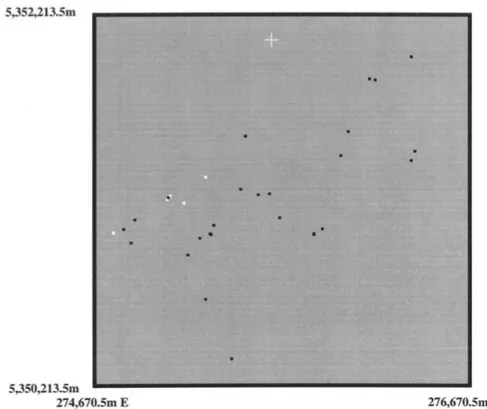
Figure 5 illustrates the location of the past landslides in a sub-area in La Baie, Quebec, Canada (Chung and Perret, 2002). The 5 white dots represent the land-slides that have occurred before 1964 and the 24 black dots are the landland-slides that have occurred in 1976 and 1996. Two of the 24 latter landslides had occurred at two of the same locations of the 5 earlier landslides. Using all the landslides that have occurred in 1964, 1976 and 1996, we have constructed a prediction model based on the likelihood ratio method (Chung and Fabbri, 1998) and a prediction pattern of the image is shown in Figure 6a.
To interpret the prediction results in Figure 6a with respect to the landslides to come during the next 35 years, we have obtained the prediction-rate curve shown in Figure 7. To generate the curve, we have generated the second prediction image
Figure 5. The distribution of landslides in part of the La Baie study area in Quebec, Canada. The 5 white dots locate the landslides of the year 1964; the 24 black dots those of 1976 and 1996.
based on the same likelihood ratio model using the 5 landslides that have occurred in 1964. This second prediction pattern based on five 1964 landslides is shown in Figure 6b and it was compared with the 24 landslides that have occurred in 1976 and 1996 to generate the “prediction-rate curve” shown in Figure 7. Although the prediction-rate curve was obtained from Figure 6b, it should be used to interpret the prediction in Figure 6a.
Ideally the tangents (slopes) of prediction-rate curves should be monotonic-ally decreased, but the empirical prediction-rate curves from the cross validation methods don’t usually satisfy the condition, as is the case in Figure 7. From the prediction-rate curve, the slope of the curve in a given prediction class is, in fact, the ratio of effectiveness defined in (1). From the prediction-rate curve in Figure 7, the ratios of effectiveness (the slopes) for several selected prediction classes were computed and shown in Table I. If the prediction-rate curve satisfies the tangent monotone decreasing condition, then the ratios of effectiveness should be also monotonically decreasing, from the most hazardous class to the least hazardous class.
From Table I, only three classes, 0–2.5%, 2.5–5% and 50–100% in Figure 6.a are significantly effective classes and 5–10% is reasonably effective prediction
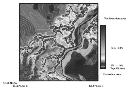
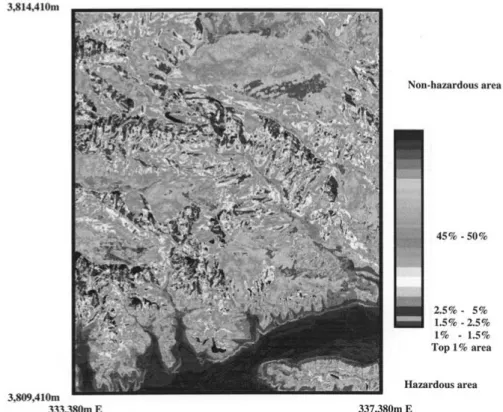
Figure 6a. Prediction pattern in the La Baie area, Quebec, obtained by the likelihood method using all the 29 landslides (both white and black dots) of 1964, 1976 and 1996.
Figure 6b. Prediction pattern in the La Baie area, Quebec, obtained by the likelihood method using only the 5 landslides (white dots) of 1964, also shown in Figure 5. The landslides of 1976 and 1996 (black dots) are used to evaluate the prediction.
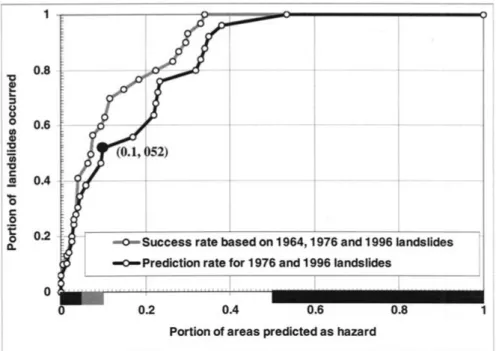
Figure 7. Prediction- and success-rate curves for the La Baie study area, Quebec. The suc-cess-rate curve was obtained by comparing Figure 6a and the 29 landslides that have occurred in 1964, 1976 and 1996. The prediction-rate curve was obtained by comparing Figure 6b and the 24 landslides that have occurred in 1976 and 1996. To interpret the Figure 6a, the prediction-rate curve, not the success-rate curve should be used. As shown in Table 1, the pre-diction classes within the black and gray bars in the X-axis are the significantly and reasonably, respectively effective prediction classes.
Table I. Ratios of effectiveness for sev-eral selected prediction classes in Figure 6a. The corresponding prediction-rate curve is shown in Figure 7
Classes Ratio of effectiveness: qt/rα 0–0.025 7.32 0.025–0.05 6.96 0.05–0.1 3.22 0.1–0.2 0.72 0.2–0.3 1.99 0.3–0.4 1.73 0.4–0.5 0.28 0.5–1.0 0.02
class. All other classes in between 10–50% don’t provide enough information for the prediction of future landslides for the next 35 years.
In contrast with the prediction-rate curve, the “success-rate curve” in Figure 7 was obtained by comparing the prediction image in Figure 6a and the distribution of all the 27 landslides that have been used to generate Figure 6a. More discussion on the prediction- and success-rate curves will be made later.
To validate a prediction image for future events,time partitioning is the most natural and convincing strategy and hence we recommend it in practice whenever possible. We can easily generalize these two partitions to several time periods.
7.1. SPACE PARTITION
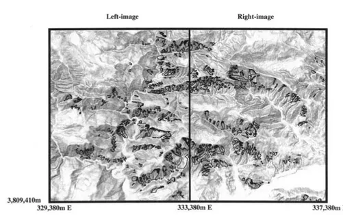
Here we also assume that we have obtained the distribution of the past landslides over the entire study area. We divide the entire study area into two separated sub-areas, A and B. We select one of two sub-areas to construct a prediction model and the other to validate the prediction. When we use this space-partition technique, then we are able to extend the current prediction model in the study area to the surrounding areas or similar geologic areas. To illustrate the procedure, we have chosen a small area in the Northridge landslide study by Chung and Jibson (2002), which is shown in Figure 8. There are 331 and 314 landslides induced by the 1996 Northridge earthquake in the “left-image” and the “right-image” in Figure 8, respectively. In that illustration, we have selected the “left-image” as a study area. A prediction model is constructed based on the study area A (left-image) including the past landslides in A. The prediction image is generated in B using the model built from A. The prediction image in B (right-image) is now compared with the distribution of the landslides occurrences of B.
In the Northridge landslide prediction study, we had used three images of slope angles, aspects and elevations of a 10 m×10 m resolution DEM and the bedrock geology map information. Using the likelihood ratio model as in the time partition case, (Chung and Fabbri, 1998) we have constructed a “left” prediction model based on the quantitative relationships between 331 landslides and the three DEM images and bedrock geology in the left-image. Based on the left prediction model, we have generated a “from-left” prediction image using the three DEM images and the bedrock geology in the “right-image”. A prediction pattern using the ranking equal number classes from the “from-left” prediction image was obtained and is shown in Figure 9a. In the illustration we have also overlaid the 314 landslides that had occurred in it. The comparison between the 314 landslides and “from-left” prediction image in Figure 9a provides the statistics and the prediction-rate curve shown in Figure 10 to evaluate the “from-left” prediction model.
In contrast with the prediction pattern in Figure 9a, we have constructed a “right” prediction model and the prediction pattern shown in Figure 9b based on the quantitative relationships between 314 landslides and the three DEM images and bedrock geology in the right-image. In Figure 9b we have then overlaid the
Figure 8. Distribution of landslide scars (bodies) and scarps (trigger areas) in part of the Northridge study area of California (USA), here subdivided into a left image and a right image. The background is a shaded relief image.
314 landslides that have used for the “right” prediction model and image. The comparison provides the statistics to evaluate the “right” prediction model. The right prediction model and the corresponding statistics from the comparison are not really for prediction but they are for “fitting” model and statistics. Table II lists the ratios of effectiveness for the predictions in Figure 9a and the corresponding prediction-rate curve in Figure 10.
The validation is studied from the comparison. We can easily generalize these two partitions to several differentspatial partitions.
7.2. RANDOM PARTITION
Identical to the time partition, the next strategy again consists of four steps and assumes that the past landslides in parts of the study area have not yet occurred. The only difference is that here we randomly divide the past landslides into two groups, instead of two time periods. We can easily generalize these two partitions to severalrandom partitions (Fabbriet al., 2003). Another generalization can be a removal of one landslide at a time and evaluate the prediction at the removed landslide site. We repeat the evaluation for each occurrence.
8. Prediction Rate and Success Rate
In all the three partitions of landslides for the validation procedure, we have used only a part of the past landslides. In the La Baie study, only the 5 landslides that have occurred in 1964 were used to generate the prediction pattern shown in Figure
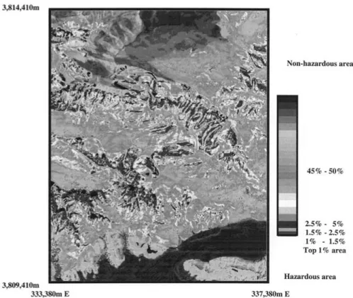
Figure 9a. Landslide hazard prediction pattern in the right sub-area obtained by the likelihood ratio method using the data from the left side sub-area in the Northridge study area, California. The distribution of the landslides shown in black was NOT used to generate this prediction. The prediction-rate curve in Figure 10 was obtained by comparing this prediction map and the landslides shown in black.
6b. By comparing the prediction results and the locations of the 24 landslides that have occurred in 1976 and 1996, we obtain the necessary statistics, which are shown as a prediction-rate curve in Figure 7. The curve is uniquely determined for each prediction image and it represents theunique measure of validationof the corresponding prediction image.
In the Northridge landslide study, instead, only the 331 landslides that have occurred in the left-image were used for prediction modelling. The comparison of the prediction image with the distribution of the 314 landslides (not used in the modelling) that have occurred in the right-image in Figure 9a generates the prediction-rate curve shown in Figure 10.
The “success-rate curve”, on the other hand, is based on the comparison between the prediction image and the landslides used in the modelling. The pre-diction pattern in Figure 9b was based on the statistical relationships between the distribution of the 314 landslides and the three DEM images and the geological map information in the right-image. The success-rate curve was obtained by the
Figure 9b. Landslide hazard prediction pattern in the right sub-area obtained by the likelihood ratio method using the data from the right side sub-area in the Northridge study area, Califor-nia. The distribution of the landslides shown in black was used to generate this prediction. The success-rate curve in Figure 10 was obtained by comparing this prediction map and the landslides shown in black.
comparison between the 314 landslides and the prediction pattern in Figure 9b. The two curves for the Northridge study are shown in Figure 10.
While the success-rate measures a goodness of fit assuming that the model is “correct”, the prediction rate provides thevalidationof the prediction regardless of the prediction model. Because we assume that the model is correct, we expect that the success rate is better than the prediction rate for any given study, as can be seen in both Figures 7 and 10.
To interpret the curve for a prediction image, consider a point (0.1,0.52) on the curve in Figure 7. For future landslides, if we take the most hazardous 10% area (0.1) of the corresponding prediction image in Figure 5, then we are estimating that 52% (0.52) of all future landslides within thenext 35years will be located in the delineated area. Therefore, if we wish to delineate areas, which should identify at least 52% of the future landslides to come within thenext 35 years, then we must declare 10% of the study area (purple and pink colored areas) a hazardous area (Figure 6a). As also shown in Table II, these areas are the effective prediction classes.
Figure 10. Prediction- and success-rate curves for the right-side sub-area. Landslide hazard prediction pattern in the right sub-area obtained by the likelihood ratio method using the data from the left side sub-area in the Northridge study area, California. The success-rate curve was obtained by comparing Figure 9b and the landslides that have occurred in the right-side sub-area. The prediction-rate curve was obtained by comparing Figure 9a and the landslides that have occurred in the right-side sub-area. To interpret the Figure 9a, the prediction-rate curve, not the success-rate curve should be used. As shown in Table II, the prediction classes within the black and gray bars in the X-axis are the significantly and reasonably, respectively effective prediction classes.
It is extremely important to notice that the prediction-rate curve relates ob-viously to the number of the future landslides and to the probability of the occurrences of future landslides. As discussed in Chung and Fabbri (2002), if we wish to link the prediction-rate curve to the probability statement regarding the occurrences of the future landslides, then we must make further assumption on the number and the size of future landslides expected within the next 35 years in the study area.
If a prediction image was generated randomly, then the prediction-rate curve should be the straight line connecting two points, (0, 0) and (1, 1). The slope of the straight line is constantly 1 and hence the ratios of effectiveness of the all prediction classes are also 1. If a prediction image has any significance, then the prediction-rate curve should be far above the straight line. It implies that if the most hazardous 10% area in Figure 6a was selected randomly, then this 10% area should predict only 10% of the future landslides, not the 52% shown in Figure 7.
Table II. Ratios of effectiveness for sev-eral selected prediction classes in Figure 9a. The corresponding prediction-rate curve is shown in Figure 10
Classes Ratio of effectiveness: qt /rα 0–0.025 9.96 0.025–0.05 8.16 0.05–0.075 3.32 0.075–0.1 3.72 0.1–0.2 0.8 0.2–0.3 0.35 0.3–0.4 0.23 0.4–0.5 0.01 0.5–0.6 0.25 0.6–0.7 0.85 0.7–0.8 1.15 0.8–1 0.035 9. Concluding Remarks
This contribution has presented strategies for validating the results of models of hazard as functions of a multi-layered spatial database. The importance of valid-ating the results of predictions, however, is broader than the specific application example here considered. Confirmation of the significance of the model results is critical in all spatial data analyses for which decisions are expected on a multi-purpose use of space for human activity. For landslide hazard, in addition, the usage of the stability of the prediction rates through time is of a far from trivial significance and warrants extensive research in many case studies and regions in different climates and geologic settings.
We have discussed examples of time, space and random partitions of the past events. They correspond to different data-dependent predictions and therefore provide distinct types of prediction patterns and of corresponding interpretations. As a consequence of applying a validation strategy, the requirements become ex-plicit of the data for prediction models. The added value of the data resides on the prediction-rate curve that also represents the efficiency of the prediction classes of the prediction patterns.
What has become evident is that the strength and therefore the reliability of a prediction can only be based on the previous prediction rates. When looking into the future, only that strength allows us to take the responsibility of making statements on what is likely to happen. When considering the spatial distribution
of the predicted relative hazard intensities, only that strength can prioritize spatial decisions.
We might have a broader expertise or a deeper intuition, however, we are unable to prove or convince that such a non-validated prediction is any better than another. The strategy proposed in this contribution wants to set up the terms to correctly apply quantitative models to generate, visualize and validate predictions by parti-tioning the database in time or in space. Ranking is the analytical technique for assessing and empirically comparing the results of the different predictions. Such results, evidently, are only meaningful in relative terms.
References
Carrara, A., Cardinali, M, Guzzetti, F., and Reichenbach, P.: 1995, GIS technology in mapping land-slide hazard, In: A. Carrara and F. Guzzetti (eds.),Geographic Information Systems in Assessing Natural Hazards, Kluwer, Dordrecht, pp. 125–175.
Chung, C. F. and Fabbri, A. G.: 1993, The representation of geoscience information for data integration,Nonrenewable Resources,2-2, 122–139.
Chung, C. F., Fabbri, A. G., Van Westen, C. J.: 1995, Multivariate regression analysis for land-slide hazard zonation, In: A. Carrara and F. Guzzetti (eds),Geographic Information Systems in Assessing Natural Hazards, Kluwer, Dordrecht, pp. 107–133.
Chung, C. F. and Fabbri, A. G.: 1998, Three Bayesian prediction models for landslide hazard, In: A. Bucciantti (ed.),Proceedings of International Association for Mathematical Geology 1998 Annual Meeting (IAMG’98), Ischia, Italy, pp. 204–211.
Chung C. F. and Fabbri, A. G.: 1999, Probabilistic prediction models for landslide hazard mapping,
Photogrammetric Engineering and Remote Sensing65-12, 1389–1399.
Chung, C. F. and Fabbri, A. G.: 2001, Prediction model for landslide hazard using a Fuzzy set Approach, In: M. Marchetti and V. Rivas (eds), Geomorphology and Environmental Impact Assessment, Balkema, Rotterdam, pp. 31–47.
Chung, C. F. and Fabbri, A. G.: 2002, Modeling the conditional probability of the occurrence of future landslides in a study area characterized by spatial data,Proceedings of 2002 ISPRS (Inter-national Society for Photogrammetry and Remote Sensing) Meeting, Ottawa, Canada, July, 2002, in press.
Chung, C. F. and Jibson, R. W.: 2002, Quantitative prediction model for landslides hazard in the Northridge area, California, in preparation.
Chung, C. F. and Perret, D.: 2002, Landslide hazard mapping in La Baie, Quebec, Canada, in preparation.
Jibson, R. W., Harp, E. L., and Michael, J. A.: 1998, A method to produce probabilistic seismic landslide hazard maps. In: A. Bucciantti (ed.), Proceedings of International Association for Mathematical Geology 1998 Annual Meeting (IAMG’98), Ischia, Italy, pp. 211–217.
Leroi, E.: 1996, Landslide hazard – Risk maps at different scales: Objectives, tools and developments, In K. Senneset (ed.),Landslides. Balkema, Rotterdam, pp. 35–51.
Packard N. H. and Wolfram S.: 1985, Two-dimensional cellular automata,Journal of Statistical Physics38, 901–946.
Panizza, M., Corsini, M., Soldati, M., and Tosatti, G.: 1998, Report on the use of new landslide susceptibility mapping techniques, In: J. Corominas, J. Moya, A. Ledesma, J. A. Gili, A. Loret, and J. Rius (eds), New Technologies for Landslide Hazard Assessment and Management in Europe (NEWTECH). Final Report, October 1998 of CEC Environment Programme Contract ENV-CT96-0248, UPC, Barcelona, pp. 13–31.
Terlien, M. T. J., Van Westen, C. J., and van Asch, T. W. J.: 1995, Deterministic modeling in GIS-based landslide hazard assessment, In: A. Carrara and F. Guzzetti (eds),Geographic Information Systems in Assessing Natural Hazards, Kluwer, Dordrecht, pp. 57–78.
Van Westen, C. J.: 1993,GISSIZ: Training package for geographic information systems in slope instability zonation. Volume 1 – Theory, International Institute for Aerospace Survey and Earth Sciences (ITC) Publication N. 15, 245 pp.
Varnes D. J.: 1984,Landslides Hazard Zonation: A Review of Principles and Practice, UNESCO, Paris, Natural Hazards, Vol. 3, 63 pp.
Wang, S.-Q. and Unwin, D. J.: 1992. Modeling landslide distribution on loess soils in China: an investigation,International Journal of Geographic Information Systems6-5, 391–405.
Zêzere, J. L.: 1996a, Landslides in the North of Lisbon region, In: A. B. Ferreira and G. T. Vieira (eds),Fifth European Intensive Course on Applied Geomorphology – Mediterranean and Urban Areas, Departamento de Geografia, Universidade de Lisboa, pp. 79–89.
Zêzere, J. L.: 1996b, Mass movements and geomorphological hazard assessment in the Trancao valley, between Bucelas and Tojal, In: A. B. Ferreira and G. T. Vieira (eds),Fifth European Intensive Course on Applied Geomorphology – Mediterranean and Urban Areas, Departamento de Geografia, Universidade de Lisboa, pp. 101–105.