Computational intelligence methods for predicting fetal outcomes from heart rate patterns

Masters Theses Student Theses and Dissertations

Spring 2018

Computational intelligence methods for predicting fetal outcomes

Computational intelligence methods for predicting fetal outcomes

from heart rate patterns

from heart rate patterns

Vinayaka Nagendra Harikishan Gude Divya Sampath

Follow this and additional works at: https://scholarsmine.mst.edu/masters_theses Part of the Systems Engineering Commons

Department: Department:

Recommended Citation Recommended Citation

Gude Divya Sampath, Vinayaka Nagendra Harikishan, "Computational intelligence methods for predicting fetal outcomes from heart rate patterns" (2018). Masters Theses. 7761.

https://scholarsmine.mst.edu/masters_theses/7761

This thesis is brought to you by Scholars' Mine, a service of the Missouri S&T Library and Learning Resources. This work is protected by U. S. Copyright Law. Unauthorized use including reproduction for redistribution requires the permission of the copyright holder. For more information, please contact [email protected].

COMPUTATIONAL INTELLIGENCE METHODS FOR PREDICTING FETAL OUTCOMES FROM HEART RATE PATTERNS

by

VINAYAKA NAGENDRA HARIKISHAN GUDE DIVYA SAMPATH

A THESIS

Presented to the Faculty of the Graduate School of the MISSOURI UNIVERSITY OF SCIENCE AND TECHNOLOGY

In Partial Fulfillment of the Requirements for the Degree MASTER OF SCIENCE IN SYSTEMS ENGINEERING

2018

Approved by Steven Corns, Advisor

Suzanna Long Ruwen Qin

© 2018

VINAYAKA NAGENDRA HARIKSIHAN GUDE DIVYA SAMPATH ALL RIGHTS RESERVED

ABSTRACT

In this thesis, methods for evaluating the fetal state are compared to make predictions based on Cardiotocography (CTG) data. The first part of this research is the development of an algorithm to extract features from the CTG data. A feature extraction algorithm is presented that is capable of extracting most of the features in the SISPORTO software package as well as late and variable decelerations. The resulting features are used for classification based on both U.S. National Institutes of Health (NIH) categories and umbilical cord pH data. The first experiment uses the features to classify the results into three different categories suggested by the NIH and commonly being used in practice in hospitals across the United States. In addition, the algorithms developed here were used to predict cord pH levels, the actual condition that the three NIH categories are used to attempt to measure. This thesis demonstrates the importance of machine learning in Maternal and Fetal Medicine. It provides assistance for the obstetricians in assessing the state of the fetus better than the category methods, as only about 30% of the patients in the Pathological category suffer from acidosis, while the majority of acidotic babies were in the suspect category, which is considered lower risk. By predicting the direct indicator of acidosis, umbilical cord pH, this work demonstrates a methodology to achieve a more accurate prediction of fetal outcomes using Fetal Heartrate and Uterine Activity with accuracies of greater than 99.5% for predicting categories and greater than 70% for fetal acidosis based on pH values.

ACKNOWLEDGMENTS

I am forever grateful to Dr. Steven Corns, my thesis advisor, for his guidance, support, and patience throughout this research.. I am very thankful for the invaluable knowledge and sense of discipline he has ingrained in me. I am thankful for the generous financial support he has provided me all throughout, in the form of a research assistantship. I would like to express my heartfelt thanks to Dr. Suzanna Long for serving on my thesis committee and for her cooperation in my research. Her support during the research was inspirational and educational. I would also thank Dr. Ruwen Qin for the honor of having her on my committee. I would like to thank Dr. James Davison for his continuous support in helping me figure out the medical terms and understand the impact of different variables on fetal asphyxia I must express my gratitude to the Ozark Biomedical Initiative, in association with the Phelps County Regional Medical Center, Rolla, MO, USA for partially funding this research.

I would like to thank all the EMSE department staff and faculty for everything they have done during my studies. I would like to thank my research colleagues Ebin, Bahnu Akhilesh and Liz. Finally, I would like to thank my family. I could not have accomplished any of this work without my parent’s care and support. Their motivation and sacrifice for my well-being have been immense. I express my deepest gratitude to them from my bottom of my heart.

TABLE OF CONTENTS

Page

ABSTRACT ... iii

ACKNOWLEDGEMENTS ... iv

LIST OF ILLUSTRATIONS ... vii

LIST OF TABLES ... viii

SECTION 1. INTRODUCTION ... 1

1.1. FETAL MONITORING TECHNIQUES ... 2

1.2. CTG CLASSIFICATION ... 4

2. ALGORITHMS ... 6

2.1. SUPPORT VECTOR MACHINE ... 6

2.2. RANDOM FOREST ... 8

2.3. LOGISTIC REGRESSION ... 11

3. CLASSIFCATION OF CTG DATA FROM UCI REPOSITORY ... 13

3.1. LITERATURE REVIEW ... 13 3.2. DATASET ... 14 3.3. RESULTS ... 15 3.3.1. Experiment One ... 15 3.3.2. Experiment Two ... 18 3.3.3. Experiment Three ... 19

4. FEATURE EXTRACTION AND CLASSIFICATION OF PCRMC DATA ... 23

4.1. LITERATURE REVIEW ... 23

4.2. PCRMC DATA ... 25

4.4. CLASSIFICATION OF CTG DATA ... 29

5. CONCLUSION AND FUTURE WORK ... 32

APPENDIX ... 34

BIBLIOGRAPHY ... 38

LIST OF ILLUSTRATIONS

Figure Page

2.1. Support Vector and Hyperplanes ... 8

2.2. Correctly and Wrongly classified data points ... 9

2.3. Random Forest ... 10

2.4. Prediction Methodology from a Random Forest ... 10

2.5. Logistic Function ... 12

3.1. Methodology for Experiment 3 ... 20

4.1. Raw Data ... 25

4.2. Data after smoothing ... 25

4.3. Raw data file ... 26

4.4. Baseline Estimation ... 26

LIST OF TABLES

Table Page

3.1. CTG Features ... 16

3.2. Performance Measures ... 17

3.3. Experiment 1 results ... 17

3.4. Experiment 1 results: Confusion Matrix(SVM) ... 18

3.5. Experiment 1 results: Confusion Matrix(RF) ... 18

3.6. Experiment 2 results ... 18

3.7. Experiment 2 results: Confusion Matrix (SVM) ... 19

3.8. Experiment 2 results: Confusion Matrix (RF) ... 19

3.9. Feature Ranking ... 21

3.10. Experiment 3 results ... 22

3.11. Experiment 4 results ... 22

4.1. Classification Accuracy for SVM and RF ... 30

4.2. Confusion Matrix SVM ... 30

4.3. Confusion Matrix RF ... 30

1. INTRODUCTION

The goal of using machine learning for classification is to make a prediction for the response variable based on the past observations. Regression is the most common technique used for this purpose. The process includes collecting the data, developing a model and analyzing the data using model to make relevant predictions. Advances in the field of Machine Learning and Computational intelligence have made it possible for machines (computers) to be more than mere calculators; they are can be trained to learn from data and make predictions based on what they have learned.

Machine Learning is defined as an application of the field of computer science, especially artificial intelligence, that can provide systems the capability to learn from data. Techniques and algorithms in the field of artificial intelligence have become an essential and capable tool for analyzing large amounts of complicated data. This has made it possible forscientists and researchers to make breakthroughs in many fields of technology and sciences. One application of machine learning is to make predictions based on collected data providing insights on the patterns within that data.

The objective of the machine learning application used here is to find a structured way of predicting an outcome given a set of observations. In artificial intelligence terms this goal is achieved by developing a supervised learning algorithm to interprete patterns from available information. Once trainined this algorithm can predict the value of a dependent variable based on the values of given independent variables. To develop a suitable model we must assume that there is a relationship between the variables. The goal of the thesis is to provide an analysis of

the feature extraction and prediction algorithms for fetal hypoxia and to provide alternatives to these algorithms. In addition, features will be analyzed to determine the most influential ones for the predictions and compared to those used in an automated commercial software package Sisporto [12]. This will be done in four steps:

(a) Analyze the data set to determine the nature of the problem. (b) Identify the most important features.

(c) Extract these important features and other recommended features. (d) Formulate a methodology for using the features and making the

predictions.

To understand the problem an introduction to fetal monitoring is necessary.

1.1. FETAL MONITORING TECHNIQUES

Approximately 25 infants out of 1000 births are affected with fetal asphyxia associated with metabolic acidosis [1]. In the majority of such pregnancies, mild oxygen deprevation to the fetus occurs with no brain harm or cerebral damage. However, in approximately 3 to 4 of these infants the hypoxia can be moderate to severe, with a few organ system complications and possible neonatal encephalopathy [1]. The objective of fetal monitoring techniques is to reduce the occurrence of mild fetal asphyxia and to prevent moderate and severe asphyxia.

It was pointed out in 1903 by Williams [29] that the evaluation of fetal heart rate variation gives us a fairly reliable means of estimating the wellbeing of the child. A general rule is that the life of the infant be considered to be at risk when the heart rate falls below 100 or exceed 160[2]. This contribution leads to the development of monitoring techniques of fetal heart rate to assess it’s well-being.

Fetal monitoring can be performed by several methods depending on the pregnancy, delivery type and risk associated with previous deliveries. Auscultation is the oldest technique involving listening to the fetus heartbeat using a stethoscope. An ultrasound captures and converts the sound waves from the mother’s abdomen into signals, which are interpreted as fetal heartbeats. Though this technique is very successful, it isn’t feasible as an experienced clinician has to stay with the patient.

Fetal scalp blood sampling involves introducing an endoscope after the dilation of the cervix. The device is firmly pressed to the scalp of the fetus and an incision is made to collect a drop a blood for measuring the pH. The placenta provides oxygen to the fetus. As umbilical cord compresses, blood flow decreases altering the oxygen levels in the fetus. This technique can be used to identify acidosis.

Electronic Fetal Monitoring is the most important medical procedure used to predict and diagnose fetal asphyxia and acidosis. It is a procedure in which electronic equipment is used to continuously track heart rate of the fetus and the uterine contractions of the mother during labor, together known as Cardiotocography (CTG). An electrode can also be used to record the signals by attaching it to the scalp of the fetus. This is one the most accurate methods for monitoring, recording and extracting the fetal heart rate with less noise. It documents an ongoing Fetal Heart Rate and when interpreted by an obstetricians gives strong indication of fetal health. Computer-aided analysis of CTG data yields a consistent and quantitative evaluation and is also capable of evaluating parameters that are difficult to be captured by the human eye. Electronic Fetal Monitoring came into existence in 1970’s and Cardiotocography was the technique used by the obstetricians for antepartum and intrapartum fetal monitoring. It records Fetal Heart Rate(FHR) and

Uterine Contractions(UC) continuously when the patient is in labor. These signals help in the assessment of the fetal state identifying hypoxic situations.

The FHR and UC readings were visually analyzed by the obstetricians to identify Metabolic Acidosis and Hypoxic injury[5], which in a few cases can lead to misdiagnosis due to varied interpretations and highly dependant on the clinician’s experience[6-10]. It can be prevented using a clinical decision support systems for diagnosis. The CTG readings can provide more information than that can be evaluated and interpreted visually by obstetricians[11]. It was reported that almost 50% of the deaths occurring during labor are due to improper diagnosis[12].

1.2. CTG CLASSIFICATION

The standard for evaluating FHR and uterine contraction patterns from the CTG is proposed by the National Institute of Child Health and Human Development. Listed below are few of the most important features for classifying CTG data.

Baseline: The mean value of Fetal Heart Rate data for a 10 min period excluding acceleration or decelerations is defined as the baseline ranging from 100 to 160 bpm.

Variability: The range of variation in the FHR excluding the acceleration or decelerations is defined as the Variability. It can be either short term or long term depending on the time.

Accelerations and Decelerations: An increase in FHR of greater than 15 beats per minute from baseline and lasting at least 15 seconds or higher is defined as an acceleration. drop in FHR of greater than 15 bpm from baseline and lasting at least 15 seconds or more is defined as an acceleration. Drop in Fetal Heart Rate shortly afterward the onset of a Uterine contraction with peaks of the deceleration and

contraction facing each other is defined as an early deceleration. It is an indication of a healthy fetus.

Late Decelerations: Onset of the deceleration starting at least 30 seconds after the onset of Uterine contraction and terminating after the contraction is defined as late deceleration.

Variable Decelerations: This is the most common type of decelerations. It can be visualized by an abrupt decrease in the FHR. It can be complicated if variable deceleration lasts for more than 60 seconds with a slow recovery to the baseline.

Prolonged Decelerations: Non-periodic decelerations lasting more than 2min and less than 10min is defined as prolonged deceleration. Explain Sisporto

Categories for Fetal Asphyxia based on FHR readings:

Category I FHR tracings include baseline FHR ranging from110 to 160 with moderate variability. They lack variable and late decelerations, with a possibility of early decelerations and accelerations.

Category II tracings are the ones that cannot be interpreted as either Category I or Category III. These readings contain: minimal or lack of variability, recurring decelerations, accelerations even after fetal movement, recurring variable decelerations with minimum baseline variability.

Category III Fetal Heart Rate readings are not normal and have a higher risk of fetal hypoxia and acidemia. They have either recurrent late decelerations or no baseline variability, or sinusoidal pattern. These readings are unusual.

2.ALGORITHMS

The objective of a supervised machine learning is to build a model or an algorithm capable of making predictions based on past observations. The model construction process included three stages: assessment of independent variable importance, identification of optimal variable sets, and model parameter tuning.

Supervised learning in general consists of classification and regression problems. For classification, the aim is to predict a class (or label) from a set of classes to an observation or given data point. The output is categorical variable. Supervised learning is prevalent in most modern technologies ranging from search engines, image classification, and anomaly detection.

For regression, the objective is to estimate and forecast a continuous measurement for an observation. The output variables are real numbers. It can be used for stock price forecasting, power consumption, temperature prediction and disease occurrence. If the output variable is a category, then it is classification and if the output variable is a real number, it is a regression.

Supervised learning is used to develop a mapping for input variables (x) and labeled output variable (Y) using an approximation function. Many machine learning techniques are appropriate for this type of analysis.

Y = f (X) (1)

2.1. SUPPORT VECTOR MACHINE

Support Vector Machine is one of the most prominent supervised learning techniques used for classifying data. It maps inputs to the outputs of the training data using hyperplanes forming a generalized model which can be used for classifying future values. Kernel methods have a kernel function that provides a mapping of

training data into feature space, on which the classification is performed. For a binary classification of classes positive and negative, the equation for the separating plane is given by,

w . x = γ (2)

where w - weights, x - input features and γ - threshold For values with positive class, w_{. xpos =} γ +1 (3)

For values with negative class, w_{. xneg =} γ−1 (4)

Distance between both these planes is given by, margin = 2/∥w∥ (5)

min∥w∥2 +µ∥s∥ (6)

w_{. xposi + si =} γ + 1 (7)

w_{. xnegj} − _{sj =} γ−1 (8) By introducing the slack variables, the objective function for the Support Vector machine is given inequation (6), where w - input feature µ - scaling constant and ⃗s - slack variable.

Support Vector Machine uses a flexible representation of the class boundaries to solve classification problems. The aim is to develop a classifier capable of working well even one unseen examples, i.e. it generalizes well.

If the classes are positive and negative, (get mathematical formulation), then the data is separable if a hyperplane can divide the n-dimensional feature space(n = number of features) into two halves. It completely separates the positive and negative classes. The hyperplane that maximizes the margin, or which has maximum separation between the classes is selected. If it is inseparable, other kernels and changing the margin boundary values.

Figure 2.1. Support Vectors and Hyperplanes[3]

The hyperplanes and Incorectly classified data points can be seen in Figures 2.1 and 2.2 respectively.

2.2. RANDOM FOREST

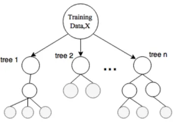
Classification and Regression Tree (CART) is a repetitive partitioning supervised learning algorithm. It makes no assumptions about the data distribution. Random Forest involves building an ensemble of CART(Classification and Regression trees) developed from a randomized variant of the tree induction algorithm. Decision trees are perfect for Random Forest as they have lower bias and higher variance.

In machine learning, random forests have been mainly applied to classification tasks due to its fast training and predictions, generalization ability and scalability. It capable of handling multiple classes due to its probabilistic output. In the below figure, a representation of different trees built from the same dataset can be seen.

for regression and majority is calculated for classification. For any event A ⊂ Ω of the sample space, the Indicator function, I is defined by,

IA(x) = 1, if x εA else 0 (9)

Assuming there are n samples in the data with d features and classes C1 and C2

.

Figure 2.2. Correctly and Wrongly classified data points[3]

It can be represented by

D = {(x1, y1), (x2, y2), ...., (xn, yn)} (10)

Assuming there are S samples at the current node that need to be partitioned.

P (Sj) = lSjl / lSl (11)

P (Cj /Sj) = lSj ∩ Cj l / lSjl (12)

g(Sj) = Σ P (Cj /Sj)(1 - P (Cj /Sj)) (13)

Variation g(Sj ) is largest if set Sj is equally divided among Cj . It’s smallest

when all of Sj is just one of the Sj . The top node contains all of the samples (xk, yk),

and the set of samples is subdivided among the children of each node until every node at the bottom has samples which are in one class only. At each node, feature xjand

threshold a are chosen to minimize resulting ’diversity’ in the children nodes. This diversity is often measured by Gini criterion.

Figure 2.3. Random Forest

If S1 and S2 are the splits, Gini Index (G) is defined by,

G = P (S1)g(S1) + P (S2)g(S2) (14)

Final prediction(y) is the majority of the outputs from the trees, as it is a classification problem. Over-fitting is a common problem with Random Forest. If a tree is split for sufficient times, it would be able to predict every single case, however, it does not summarise data thus is of no use predicting cases in a new dataset.

As a general rule, we should stop splitting the tree when more splits contribute little to the overall performance of the prediction. Representation and classification of data can be seen in Figures 2.3 and 2.4 respectively.

2.3. LOGISTIC REGRESSION

Logistic regression is a statistical method for evaluating a dataset in with one or more input variables that determine the value of an output variable. The objective of this algorithm is to find the best fitting model to describe the relationship between the dependent variable and the given set of independent variables.

A logistic function is an ’S’ shaped curve as shown in the figure below that maps real-value numbers to values between 0 and 1. It is mathematically, represented by,

f(x) =1 / (1 + e-x) (15) Logistic Regression can be represented using the below equation,

y = e b0 + b1 * x / ( 1 + e b0 + b1 * x) (16) where b0 - bias or intercept and b1 - coefficient of input term(x). For a

classification problem, assuming the classes 1 and 2 for a given data.

p(X) = p(Y = 1|x) = e b0 + b1 * x / ( 1 + e b0 + b1 * x) (17) Where p(X) - probability that X belongs to class (Y=1) Rearranging and

applying natural logarithm(ln) to the above function we get,

ln (p(X)/1 – p(X)) = b0 + b1 * x (18) Logistic regression makes similar approximations regarding the data distribution and relationships in between input and output variables are similar to that of linear regression. So logistic regression gives us a linear classifier.

3. CLASSIFICATION OF CTG DATA FROM UCI REPOSITORY

3.1. LITERATURE REVIEW

A body of research has been performed by various hospitals and researchers to develop algorithms which can capture all the information. Various Machine Learning techniques such as Artificial Neural Networks, Fuzzy Systems, Genetic algorithms, Support Vector Machines and hybrid algorithms were used on the CTG data obtained from SISPORTO 2.0.

Different computer-based CTG assessment techniques and algorithms were proposed over the years. Retrospective classification is the most common technique. One of the first models developed was an Auto-Regressive Moving Average algorithm[13], with features extracted from Fetal Heart Rate data and a linear discriminant function for classification. Computerised Cardiotocography analysis systems were developed based on guidelines provided by the International Federation of Obstetrics and Gynecology. A Neural network with back propagation was used for the classification of Non-Stress Test records and to predict fetal acidosis at birth. An Artificial Neural Network was also used to classify the fetal states 1(normal) and 3(pathological). A fuzzy rule-based expert system was introduced to handle uncertainties in FHR interpretations [14]. Wavelet analysis with self-organizing maps was used to predict fetal hypoxia based on the Fetal Heart Rate features which are scale-dependant. Hidden Markov Model(HMM) was developed with 12 time and domain features to classify hypoxic and normal states[14]. A Support Vector Machine(SVM) was implemented to identify fetuses developing acidosis[15].

Features extracted wavelets have also been used for classification. Power spectral density (PSD) of Fetal Heart Rate signal along with fuzzy systems was used

to extract features to estimate the fetal state[16]. An advanced model of the wavelet feature extraction was also developed for evaluating FHR data[17]. Non-linear features like fractal dimension, approximate entropy, and Lempel Ziv complexity were used to classify Fetal Heart Rate signals as category 1 (normal) and category 3 (pathological) using Naive Bayes, Neural and SVM classifiers[18]. Self-organizing maps were also used for fetal monitoring[19]. Adaptive neuro-fuzzy inference systems based models have a great property of being good universal approximators with a capability of interpretable IF-THEN rules, have also been used for prediction of fetal state/category from the CTG data [20].

Most of the above mentioned research included fetal categories ‘normal’ and ‘pathalogical’ leaving out the ‘suspect’ state. In reality, more than 50% of the deliveries fall under ‘Suspect’ category. A model without it, would not capture a real scenario and cannot be used in predicting real-time data. So, motive of this research is to model with all the 3 categories representing a more realistic prediction of the fetal states.

3.2. DATASET

For our initial analysis, a CTG data was acquired from University of California Irvine Machine Learning Repository and features extracted by the University of Porto using SisPorto 2.0. The features were extracted based on International Federation of Obstetrics and Gynecology guidelines. The dataset consisted of 21 features per CTG recording. 8 of the features were continuous and obtained from time series whereas the rest of them were discrete and obtained from histogram data. The dataset was used to predict the fetal state as per established categories (Normal, Suspect and Pathological) with the category validated by skilled obstetricians. A total of 2126

recording were present in the data, of which 1655 were normal, 295 were suspect and 176 were of pathological states. The different features can be seen in Table 3.1.

3.3. RESULTS

Support Vector Machine (SVM) and Random Forest (RF) were used to classify the CTG recording based on the above-mentioned features. 4 different experiments were conducted with a slight variation in the number of states and features.

Experiment 1 was performed with CTG data of all the features and classifying only normal and pathological states. This experiment was to replicate the results of fetal state prediction using SVM and RF in [11] Experiment 2 was performed with CTG data of all the features and classifying normal, suspect, and pathological states. This experiment was to determine how well these methods would work if suspect cases were included.

Experiment 3 was performed with CTG data of the most important features as identified by the Logistic Regression and Extra-trees classifier and classifying normal and pathological states. Experiment 4 was performed with CTG data of the most important features as identified by the Logistic Regression and Extra-trees classifier and classifying normal, suspect and pathological states.

Comparison of Experiments 1 and 2 depict the difference in accuracy during real-life CTG analysis with the inclusion of Suspect state. Experiment 3 after the identification of important features would improve the accuracy over Experiment 1 and Experiment 2.

3.3.1. Experiment One. For this experiment, the CTG recordings for the

Table 3.1. CTG Features[12]

SVM and the parameters gamma and c (regularization parameter) were tuned for higher classification accuracy. Kernel functions were poly,linear and RBF.

Table 3.2. Performance Measures[12]

The regularisation parameter (c) steers the bargain between the slack variable penalty (misclassifications) and width of the margin. Small ’c’ value, indicates going easy on the constraints, resulting in a large margin, whereas higher ’c’ value results in a smaller margin.

A different number of trees was tested for Random Forest for each of the experiments. Leaf size indicating end nodes can also be optimized. 5 fold cross validation was used to select the data used in the experiments. Accuracy was the performance measure used to compare the algorithms. True Positives, True Negatives, False Positives and False Negatives were calculated to evaluate the accuracy.

For Experiment 1, CTG data consisting of Normal and Pathological Fetal States were used to train and test the algorithms. Random Forest had higher Accuracy compared to Support Vector Machine for this Binary classification problem as shown in Table 3.3. The confusion matrix for SVM and RF are given the Tables 3.4 and 3.5 respectively. This experiment does not represent a real-life situation, as most of the cases fall in the Suspect category. To explore this case, all the three states were used for classification in Experiment 2.

Table 3.3. Experiment 1 results

Measure SVM RF

Table 3.4. Experiment 1 results: Confusion Matrix(SVM) Predicted Actual Normal Pathological Normal 0.99939 0.119 Pathological 0.0006 0.8806

Table 3.5. Experiment 1 results: Confusion Matrix(RF)

Predicted

Actual

Normal Pathological

Normal 0.99939 0

Pathological 0.0006 1

3.3.2. Experiment Two: For Experiment 2, CTG data consisting of Normal,

Suspect and Pathological Fetal States were used to train and test the algorithms. Cross-fold validation and parameter tuning of both SVM and RF remain same for all the experiments. Support Vector Machine performed better at classifying all the three fetal states compared to Random Forest as shown in Table 3.6. Corresponding Confusion matrices for both the algorithms are given in Table 3.7 and Table 3.8.

Table 3.6. Experiment 2 results

Measure SVM RF

Accuracy 98.122 97.289

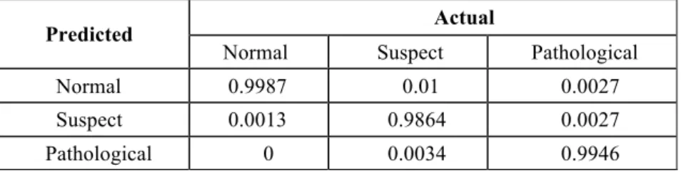
A confusion matrix is also known as Error matrix and is a measure of performance of an algorithm on classification problem with more than 2 more states. Rows represent the fraction of classes predicted by the algorithm whereas the columns represent the fractions for actual classes. It is an important measure for multi-class predictive analytics. It gives the performance of the classification model in predicting the 3 fetal states. It can be used to evaluate the sensitivity and precision for each state.

Table 3.7. Experiment 2 results: Confusion Matrix (SVM)

Predicted Actual

Normal Suspect Pathological

Normal 0.9987 0.01 0.0027

Suspect 0.0013 0.9864 0.0027

Pathological 0 0.0034 0.9946

Table 3.8. Experiment 2 results: Confusion Matrix (RF)

Predicted Actual

Normal Suspect Pathological

Normal 0.9972 0.0067 0

Suspect 0.0027 0.9898 0

Pathological 0 0.0034 1

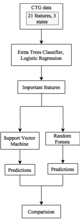
3.3.3. Experiment Three: Feature selection is useful in choosing a subset Xs

of the full set of input features Xs = {X1,X2,..., Xm} so that the selected subset Xs can effectively predict the output category/class Y with an accuracy close to the performance of the full input set X, and with lesser computational power. For this experiment, extra trees classifier and Logistic Regression were used for feature ranking.

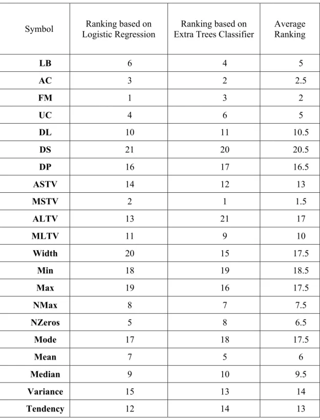
Grid Search has been used to optimize the parameters for both Support Vector Machine and Random Forest. The average rankings are presented in Table 3.9. Both the algorithms gave similar results; this ranking can help in identifying features that provide more information to predict asphyxia. Average values of both the feature rankings are calculated and sorted based on that. The least 5 impactful features (DS, Width, Min, Max, and Mode) were identified. In Experiment 3 used the identified important features for classification of two categories (normal and pathological) and Experiment 4 used the features for classification of threecategories (normal, suspect and pathological). Similar to experiments 1 and 2, Random Forest performs better for 2 category classification and Support Vector Machine has a higher accuracy when all the three states were used, as shown in Table 3.10 and Table 3.11.

Figure 3.1. Methodology for Experiment 3

Accuracy has been improved in both the cases, proving that using only important features compared can achieve better results compared to using all the features. The methodology for the experiments can be seen in Figure 3.1.

Table 3.9. Feature Ranking

Symbol _{Logistic Regression} Ranking based on _{Extra Trees Classifier} Ranking based on Average _Ranking

LB 6 4 5 AC 3 2 2.5 FM 1 3 2 UC 4 6 5 DL 10 11 10.5 DS 21 20 20.5 DP 16 17 16.5 ASTV 14 12 13 MSTV 2 1 1.5 ALTV 13 21 17 MLTV 11 9 10 Width 20 15 17.5 Min 18 19 18.5 Max 19 16 17.5 NMax 8 7 7.5 NZeros 5 8 6.5 Mode 17 18 17.5 Mean 7 5 6 Median 9 10 9.5 Variance 15 13 14 Tendency 12 14 13 21

Table 3.10. Experiment 3 results

Measure SVM RF

Accuracy 98.954 99.78

Table 3.11. Experiment 4 results

Measure SVM RF

Accuracy 99.895 99.727

4. FEATURE EXTRACTION AND CLASSIFICATION OF PCRMC DATA

4.1. LITERATURE REVIEW

Feature extraction involves gathering specific parameters/patterns from a signal/time series data that can be easier to analyze than the entire signal sample. Automated Computerized analysis of the CTG recordings decreases the subjective nature of fetal state based on visual interpretation. Information loss is inherent in most of the Computerized analysis techniques. Information loss caused by these feature extraction algorithms simplifies and reduces the complexity of the data for classification. This method showed higher accuracy in agreement with clinical experts. Different techniques and algorithms for extracting features and analysis of CTG data can be considered.

Artificial Neural Networks (ANN) with their capability of learning and generalizing, they were most prominently used for the fetal state assessment. The fetal condition was evaluated using a feedforward neural network consisting of five layers on Fetal Heart Rate signals [21].

Based on the analysis done in previous sections in identifying the important features for fetal asphyxia prediction, following are the features that we plan to extract from the data. By the addition of fuzzy logic to a current clinical expert system assessing 5-minute segments of Fetal Heart Rate signals was developed [22]. Fuzzy inference systems based classifiers of the FHR signals were developed to predict the intrauterine growth retardation and diabetes type I depending on gestational age and quantitative description of the Fetal Heart Rate data in time and frequency domain FHR analysis [23]. Artificial Neural Network with three layers and clustering using fuzzy logic were compared for over sixteen thousand FHR signals in a database with

thirty-nine parameters [24]. Fetal state assessment based on FHR data analysis was performed using an ANN combined with inference system using fuzzy logic was developed for the predicting fetal state/category based on analysis of Fetal Heart Rate signals. Epsilon-insensitive learning method based on statistical learning theory was used to obtain high prediction accuracy [25]. SVM is one of the most common algorithms known for classifying data and regression analysis. SVM was applied to predict intrauterine growth inhibition risk of the fetus and also assess the impact of the input features selection on the prediction accuracy [26]. The Support Vector Machine algorithm in combination with wavelet transformation of input features helped in achieving a higher prediction accuracy of fetal acidemia risk [27]. A Support Vector Machine algorithm combined with empirical mode decomposition was developed to achieve high compliance of Fetal Heart Rate data prediction with an expert clinical interpretation [28]. The thesis presents a new method for extracting features and evaluating fetal acidemia risk.

Though a lot of research was done in developing automated fetal assessment systems, only a few were implemented for real-time fetal monitoring. Dawes/Redman criteria algorithms [33] were developed in 1982 for CTG analysis aimed at predicting fetal state, normal or pathological. It led to the development of a system for intrapartum fetal monitoring combining CTG with ST-analysis of the electrocardiogram (ECG) named STAN S31, by Neoventa Medical [32]. It generates alarms for hypoxic conditions related to muscle contractions and lack of oxygen. Sisporto is another clinically implemented system for computerized FHR analysis. Sudden peaks and drops in the FHR readings of greater than 50 beats are assumed to be caused by the devices. A Rolling Mean is used to account for the noise.

4.2. PCRMC DATA

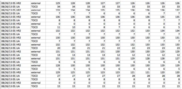
Figure 4.1. Raw Data

Cardiotocography data consists of four readings of Fetal Heart Rate and Uterine Contractions collected every second during the labor. Figure 4.1, represents raw Fetal Heart Rate for a patient. To identify the features, noise reduction is an important steps in Data Analysis. Noise in the CTG data might be due to fluctuations caused by the devices or movement of the patients.

Figure 4.3. Raw data file

4.3. FEATURES

Baseline: An algorithm for extracting features such as baseline, acceleration, deceleration, early deceleration, late deceleration, and variability was written and implemented in python.

There are a few algorithms for calculating variable baseline, but for the purpose of using it as a feature for estimation of asphyxia, a stable baseline is preferred. An iterative approach is used to estimate the baseline as defined by the FIGO guidelines. The data is split into corresponding FHR and UC level readings. The signal loss and noise in the FHR and UC data is taken care of by the smoothing. Smoothing of the signals is done using a rolling mean algorithm provided by the pandas library in python.

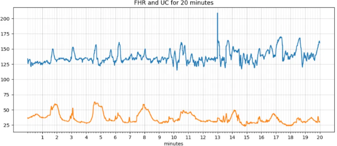
A rolling mean filter is the most common technique in Signal Processing. It is simple and optimal for reducing random noise while retaining a sharp step response. The minimum time span for CTG assessment was considered to be 20 min [32]. Mean(M) is calculated as the Baseline based on literature review as most of the early algorithms and techniques used ’mean’. Accelerations and Decelerations are estimated using this baseline as a point of comparison.

The baseline (N) is again calculated after removal of accelerations and decelerations and compared to the original baseline, to check the deviation. If the deviation is greater than 0.5, the process is repeated with New baseline (N) as the baseline.

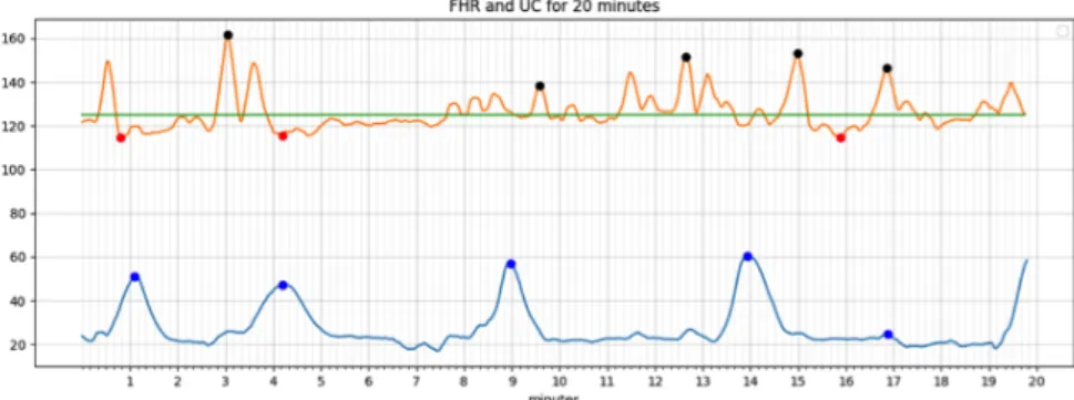
In Figure 4.5, the Fetal Heart Rate is shown in orange, Uterine contractions readings in blue and baseline are represented by green line for a 20 min window, Accelerations are represented in Black, Decelerations in Red and the Uterie Contractions in Blue. These are evaluated as mentioned below following the FICO guidelines.

Accelerations: An acceleration has a peak of at least 15 beats/min above baseline and a duration of at least 15 seconds but less than 2 minutes. The flowchart for

estimating accelerations, Baseline and Decelerations is given by the flowchart in Figure 4.4.

Decelerations: An deceleration has a fall of at least 15 beats/min below baseline and a duration of at least 15 seconds but less than 2 minutes. A Deceleration between 2 minutes and 5 minutes is defined as Prolonged Deceleration. A Deceleration lasting more than 5 minutes is called Severe Deceleration. If the deceleration starts after the peak and before the end point of the contraction and lasts more than 15 seconds and has a peak of at least 15 beats above the baseline is defined as a Late Deceleration. Contractions: Peaks of over 10 points in UC level readings and lasting 20-240 sec are defined as Contractions.Histogram data: The histogram is plotted for the Fetal Heart Rate data and Mean, Median, Mode are calculated. Minumum and Maximum values of the Histogram are identified. The width of histogram is evaluated which is the difference between the minimum and maximum values. Final class: The Classifcation parameter for the problem is Acidosis. A pH value less than 7.2 is defined as acidotic (‘1’) and greater than 7.2 is non-acidotic (‘0’).

Acidosis: The Placenta of the mother provides oxygen to the fetus and removes Carbon Dioxide. It is susceptible to changes based on the maternal blood gas concentrations, uterine blood supply, placental transfer, and the gas transport of the fetus.

Affecting any of the above processes can lead to acidosis, which can lead to significant fetal morbidity and mortality. Acidosis is indicated by a high hydroxide [OH-] concentration in the tissues. The reference range for pH values of the fetuses was obtained based on a few studies with antenatally taken blood specimen after delivery.

There are maternal, placental, or fetal causes of fetal acidosis and asphyxia. The impact of Acidosis is determined by the severity and duration of the acidosis. Maternal causes are Hypotension, vasovagal attack or epidural anesthesia [30]. Placental causes are abruption resulting in disruption of uteroplacental circulation by damaging the uterine spiral arteries. Fetal causes are disruption of the flow of blood from the placenta to the fetus by umbilical cord compression. At least 50% of blood movement to the fetus has to be affected to result in Asphyxia. Acidosis is caused due to tissue hypoxia and it is highly uncertain if the aftereffects are due to the acidosis or the hypoxia. The consequences are differing relying on if the exposure is chronic or acute. The fetus is adaptive and can even tolerate severe Hypoxia and Acidosis for shorter time periods but will be adversely affected by longer exposure. Prevention of Severe acidosis depends on the fetal monitoring techniques and the observations made the obstetricians.

4.4. CLASSIFICATION OF CTG DATA

The cutoff point for differentiating acidosis is chosen as 7.2, all the values below 7.2 are considered to acidotic and the values above are non-acidotic. Features are extracted from the data provided by GE and PCRMC based on the criteria mentioned in the Feature Extraction section.

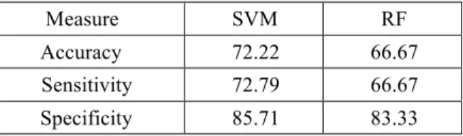
Similar to the earlier experiments, Support Vector Machine (SVM) and Random Forest (RF) were used to classify the CTG data based on umbilical cord pH values. Logistic Regression and Extra-trees classifier are then used to identify the most important features. The accuracies of SVM and RF are 72.22 and 66.67 respectively. Support Vector Machine performed slightly better than Random Forest. Of the 18 samples available for testing, SVM classified 13 correctly whereas RF did classify 12 accurately.

Table 4.1. Classification Accuracy for SVM and RF

Measure SVM RF

Accuracy 72.22 66.67

Sensitivity 72.79 66.67

Specificity 85.71 83.33

Confusion matrix for SVM and RF are given in the Tables 4.2 and 4.3 respectively. True positives, False Positives, True Negatives, False Negatives are 88.89, 33.33, 66.67 and 11.11 percent respectively for SVM whereas 88.89, 44.44, 55.55 and 11.11 percent respectively are for RF.

Support Vector Machine has higher accuracy,sensitivity and specificity compared to that of Random Forest for predicting accuracy.

Table 4.2. Confusion Matrix SVM

Predicted Actual

Acidosis(9) Non-acidosis(9) Acidosis 88.89(8) 33.33(3) Non-acidosis 11.11(1) 66.67(6)

Table 4.3. Confusion Matrix RF

Predicted Actual

Acidosis(9) Non-acidosis(9)

Acidosis 88.89(8) 44.44(4)

The overall less accuracy is due to lack of training data. Of over 8000 patients treated at Phelps County Regional Medical Center, only 47 were diagnosed with acidosis, limiting the data size to 94. The results from Feature Ranking are shown in Table 4.4. The lower the ranking of the features, higher the importance.The results were validated by a group of Obstetricians from Phelps County Regional Medical Center and Saint Louis Uninversity Hospital.

Table 4.4. Feature Ranking

Features Ranking based on Logistic _Regression

FHR Baseline 1 Accelerations 1 Decelerations 3 Uterine Contractions 4 Variable Decelerations 1 Severe Decelerations 5 Prolonged Accelerations 7 Prolonged Decelerations 6 Light Decelerations 2 Width of Histogram 1 Min. of Histogram 1 Max. of Histogram 1 No of peaks 1 Mean 1 Median 1 Mode 1 Variability 1

5. CONCLUSION AND FUTURE WORK

This research work proposes a methodology to use Cardiotocography readings of fetuses to determine if they are at risk of developing asphyxia to advise attending clinicians. Features were extracted from both the Fetal Heart Rate and Uterine Contractions data based on the medical guidelines and then Machine Learning algorithms were used for classification. In addition, cord pH data was used as the predicted state to classify CTG data, a direct indicator of fetal acidosis.

A review of the algorithms, features and classification parameters has been provided. In particular, Support Vector Machine and Random Forest for classification, Logistic Regression and Extra trees Classifier for feature importance and Fetal states and pH level for prediction. All 21 features identified by SISPORTO in the dataset available on the University of Calfornia, Irvine website were used to classify fetal states for compaison. This set of 21 features was reduced to only the most significantfeatures for prediction, improving the performance. Finally, features were extracted from the data provided by the Phelps County Regional Medical Center and used to classifiy time series data based on pH values.

Over the past 10 years, Phelps County Regional Medical Center has treated over 8000 patients with only 47 of them suffering from Acidosis, limiting the total dataset size to 94 50% positive, 50% negative), to prevent bias. The accuracy in predicting can be improved with more data. Insufficient training data (with just 94 samples) resulted in classification accuracy of 66.67 % for the Support Vector Machine and 67.33% for the Random Forest. One appraoach to overcome this small dataset would be to duplicate data (with the addition of noise) to increase training dataset size which can drastically improve the accuracy of the algorithm. The issue with such an

approach is overfitting. The algorithm would not be able to predict unseen values effectively, thereby limiting its utility. Because of this, more data is the most appropriate solution to this problem.

Future work involves obtaining more data to improve the accuracy of Support Vector Machine and Random Forest. Develop an algorithm to extract features for a 20 min window of CTG time series and use probabilistic dependencies to predict acidosis and give a progression of the fetal health. Algorithms such as LSTM or Recurrent Neural Network[34] can be used for this purpose. The above-mentioned methodology and algorithms with more data can be used to develop a real-time fetal monitoring system capable of effectively predicting acidosis based on CTG data using pH values.

APPENDIX

CODE

Classification of CTG data using Support Vector Machine and Random Forest

# Comparing Support Vector Machines and Random Forests

import csv

import numpy as np from sklearn import svm

from sklearn.ensemble import RandomForestClassifier

#Loading the data data = []

file = open('toco.csv', "r") read = csv.reader(file) for row in read : data.append(row)

# Parse the data into inputs and targets from the data file(toco.csv). arraydata = np.array(data)

inputs = np.delete(arraydata,np.s_[32],1) targets = np.delete(arraydata,np.s_[0:32],1)

# divide the data into training and testing data sets. inputs = inputs.astype(np.float)

outputs = targets.astype(np.float)

trainin, testin = inputs[:1063,:], inputs[1063:,:] trainout, testout = outputs[:1063,:], outputs[1063:,:]

trainout = np.array(trainout,np.float32).reshape(len(trainout),1) trainout = trainout.reshape(-1,1)

trainout = np.concatenate(trainout, axis=0 ) trainout = np.array(trainout) # Random Forest random_forest = RandomForestClassifier(n_estimators = 100,random_state=10000) random_forest = random_forest.fit(trainin,trainout) predict_rf = random_forest.predict(testin)

# Support Vector Machine

Support_Vector_Machine = svm.SVC(gamma=0.04, C=4,degree=3, kernel='linear')

Support_Vector_Machine = Support_Vector_Machine.fit(trainin, trainout) predict_svm = Support_Vector_Machine.predict(testin)

#reshaping testout

testout = np.array(testout,np.float32).reshape(len(testout),1) testout = testout.reshape(-1,1)

testout = np.concatenate(testout, axis=0 ) testout = np.array(testout) accurate_rf =0 accurate_svm=0 for x in range(len(predict_rf)): if predict_rf[x] == testout[x]: accurate_rf = accurate_rf+1 if predict_svm[x] == testout[x]: accurate_svm = accurate_svm+1 print (accurate_rf)

print ('The accuracy for the RandomForest is ', accurate_rf/len(testout)*100) print (accurate_svm)

print ('The accuracy for the RandomForest is ', accurate_svm/len(testout)*100)

# Identification of the most important features for prediction. # ExtraTreesClassifier for ranking the features used.

from sklearn.ensemble import ExtraTreesClassifier

model = ExtraTreesClassifier() model.fit(inputs, outputs)

print(model.feature_importances_)

# Logistic Regression to identify the 10 most important # features contributing towards the prediction.

from sklearn.feature_selection import RFE

from sklearn.linear_model import LogisticRegression

model = LogisticRegression() rfe = RFE(model, 10) fit = rfe.fit(inputs, outputs)

BIBLIOGRAPHY

[1] JA Low, BG Lindsay, EJ Derrick, Threshold of metabolic acidosis associated with newborn complications, Am J Obstet Gynecol, 177 (1997), pp. 1391-1394.

[2] Endorsed by the European Society of Gynecology (ESG), the Association for European Paediatric Cardiology (AEPC), and the German Society for Gender Medicine (DGesGM), Authors/Task Force Members, Regitz-Zagrosek, V., Blomstrom Lundqvist, C., Borghi, C., Cifkova, R., ... & Gorenek, B. (2011). ESC Guidelines on the management of cardiovascular diseases during pregnancy: the Task Force on the Management of Cardiovascular Diseases during Pregnancy of the European Society of Cardiology (ESC). European heart journal, 32(24), 3147-3197.

[3] Ocak, Hasan. "A medical decision support system based on support vector machines and the genetic algorithm for the evaluation of fetal well-being." Journal of medical systems 37.2 (2013): 9913.(SVM)

[4] Logistic function (sigmoid).png. (2017, October 15). Wikimedia Commons, the free media repository. Retrieved 02:43, February 2, 2018 from

https://commons.wikimedia.org/w/index.php?title=File:Logistic_function_(sig moid).png&oldid=263014883.

[5] Van Geijn, H.P, “Developments in CTG analysis,” Bailliere’s Clin. Gynaecol., vol. 10, no. 2, pp. 185–209, Jun. 1996.

[6] MacDonald, D., Grant, A., Sheridan-Pereira, M., Boylan, P., and Chalmers, I., The Dublin randomized controlled trial of intra- partum fetal heart rate monitoring. Am.J.Obstet. Gynecol. 152:524–539, 1985.

[7] Goddard, R., Electronic fetal monitoring is not necessary for low risk labours. Brit. Med. J. 322:1436–1437, 2001.

[8] Rooth, G., Huch, A., and Huch, R., Guidelines for the use of fetal monitoring. Int. J. Gynaecol. Obstet. 25:159–167, 1987.

[9] Bernardes, J., Costa-Pereira, A., Ayres-de-Campos, D., van-Geijn, H. P., and Pereira-Leite, L., Evaluation of interobserver agreement of cardiotocograms. Int. J. Gynaecol. Obstet. 57:33–37, 1997.

[10] Palomaki, O., Luukkaala, T., Luoto, R., and Tuimala, R., Intrapartum cardiotocography - the dilemma of interpretational variation. J Perinat Med 34:298–302, 2006.

[11] Signorini, M.G, Magenes, G, Cerutti, S, and Arduini, D, “Linear and nonlinear parameters for the analysis of fetal heart rate signal from

cardiotocographic recordings,” IEEE Trans. Biomed. Eng., vol. 50, no. 3, pp. 365–374, Mar. 2003.

[12] Ayres-de-Campos, D , Costa-Santos, C, Bernardes, J, S.M.V.S. Group, Prediction of neonatal state by computer analysis of fetal heart rate tracings: the antepar-tum arm of the SisPorto® multicentre validation study, Eur. J. Obstet. Gynecol.Reprod. Biol. 118 (2005) 52–60.

[13] Jongsma, H. W., and Nijhuis, J. G., Classification of fetal and neonatal heart rate patterns in relation to behavioural states. Eur. Obstet. Gynecol. Reprod. Biol. 21:293–299, 1986.

[14] Georgoulas, G., Stylios, C. D., Nokas, G., and Groumpos, P. P., Classification of fetal heart rate during labour using hidden Markov models. Proc IEEE Int Joint Conf. Neural Netw. 3:2471–2474, 2004.

[15] Signorini, M. G., de-Angelis, A., Magenes, G., Sassi, R., Arduini, D., Cerutti, S., Classification of fetal pathologies through fuzzy inference systems based on a multiparametric analysis of fetal heart rate. Comput. Cardiol. 27:435– 438, 2000.

[16] Georgoulas, G.,Stylios, C. D., andGroumpos,P.P., Feature extraction and classification of fetal heart rate using wavelet analysis and support vector machine. Int. J. Artif. Intell. Tools 15:411–432, 2005.

[17] Vaisman, S., Salem, S. Y., Holcberg, G., and Geva, A. B., Passive fetal monitoring by adaptive wavelet denoising method. Comput. Biol. Med. 42:171–179, 2012.

[18] Magenes, G., Signorini, M. G., and Arduini, D., Classification of

cardiotocographic records by neural networks. Proc. IEEE-INNS- ENNS Int. Joint Conf. Neural Netw. (IJCNN’00) 3:637–641, 2000.

[19] Liszka-Hackzell, J. J., Categorization of fetal heart rate patterns using neural networks. J. Med. Syst. 25:269–276, 2001.

[20] Magenes, G., Signorini, M.G., Sassi, R., Arduini, D., Multiparametric analysis of fetal heart rate: comparison of neural and statistical classifiers. Proceedings of Medicon 2001, Pula, Croatia, 360–363, (2001).

[21] Hasbargen, U. (1994). Application of neural networks for intrapartum surveillance. In H. van Geijn & F. Copray (Eds.), A critical appraisal of fetal surveillance (pp. 363–367). Amsterdam, New York: Elsevier Science. Excerpta Medica.

[22] Keith, R., Beckley, S., & Garibaldi, J. (1995). A multicentre comparitive study of 17 experts and an intelligent computer system for managing

labour using the cardiotocogram. British Journal of Obstetrics & Gynaecology, 102, 688–700.

[23] Arduini, D., Giannini, F., Magnes, G., Signorini, M. G., & Meloni, P. (2001). Fuzzy logic in the management of new prenatal variables. In Proceedings of 5th World Congress of Perinatal Medicine, Barcelona (pp. 1211–1216), vol. 1. [24] Frize, M., Ibrahim, D., Seker, H., Walker, R., Odetayo, M. O., Petrovic, D., &

Naguib, R. N. G. (2004, September). Predicting clinical outcomes for newborns using two artificial intelligence approaches. In Engineering in Medicine and Biology Society, 2004. IEMBS'04. 26th Annual International Conference of the IEEE (Vol. 2, pp. 3202-3205). IEEE.

[25] Leski, JACEK M. "The ε-insensitive learning techniques for approximate reasoning system." International Journal of Computational Cognition 1.1 (2003): 21-77.

[26] Magenes, G., Pedrinazzi, L., & Signorini, M. (2004). Identification of fetal sufferance antepartum through a multiparametric analysis and a support vector machine. In Engineering in Medicine and Biology Society, 2004. IEMBS ’04. Proceedings of 26th annual international conference of the IEEE (pp. 462– 465), vol. 1.

[27] Warrick, P., Hamilton, E., Precup, D., & Kearney, R. (2010). Classification of normal and hypoxic fetuses from systems modeling of intrapartum

cardiotocography,IEEE Transactions on Biomedical Engineering, 57, 771– 779.

[28] Krupa, N., MA, M., Zahedi, E., Ahmed, S., & Hassan, F. (2011). Antepartum fetal heart rate feature extraction and classification using empirical mode decomposition and support vector machine. BioMedical Engineering OnLine, 10, 1–15.

[29] Williams JW: Williams Obstetrics, 1st ed. New York, Appleton, 1903.

[30] Brown, VA, Sawers, RS, Parsons, RJ, Duncan, SL, Cooke, ID. The value of antenatal cardiotocography in the management of high-risk pregnancy: a randomized controlled trial. Br J Obstet Gynaecol. 1982;89:716–722.

[31] Lewis Mehl-Madrona, M. D., & Mehl-Madrona, M. Medical Risks of Epidural Anesthesia During Childbirth.

[32] Norén, H., & Carlsson, A. (2010). Reduced prevalence of metabolic acidosis at birth: an analysis of established STAN usage in the total

population of deliveries in a Swedish district hospital. American Journal of Obstetrics & Gynecology, 202(6), 546-e1.

[33] Dawes, G. S., Houghton, C. R. S., Redman, C. W. G., & Visser, G. H. A. (1982). Pattern of the normal human fetal heart rate. BJOG: An International Journal of Obstetrics & Gynaecology, 89(4), 276-284.

[34] Sundermeyer, M., Schlüter, R., & Ney, H. (2012). LSTM neural networks for language modeling. In Thirteenth Annual Conference of the International Speech Communication Association.

VITA

Vinayaka Nagendra Harikishan Gude Divya Sampath was born in Visakhapatnam, Andhra Pradesh, India. He received his Bachelor of Technology degree in Chemical Engineering from Jawaharlal Nehru Technological University in Kakinada, India.

In 2016, Vinayaka began attending Missouri University of Science and Technology (Missouri S&T) in Rolla, USA. In May 2018, Vinayaka received a Master’s degree in Systems Engineering from Missouri University of Science and Technology.