Forecasting bank loans loss-given-default
Jo˜ao A. Bastos
∗Center for Applied Mathematics and Economics (CEMAPRE) School of Economics and Management (ISEG)
Technical University of Lisbon, 1200-781 Lisboa, Portugal
This version: September 2009
Abstract
With the advent of the new Basel Capital Accord, banking organizations are invited to estimate credit risk capital requirements using an internal ratings based approach. In order to be compliant with this approach, institutions must estimate the expected loss-given-default, the fraction of the credit exposure that is lost if the borrower defaults. This study evaluates the ability of a parametric fractional response regression and a nonparametric regression tree model to forecast bank loan credit losses. The out-of-sample predictive ability of these models is evaluated at several recovery horizons after the default event. The out-of-time predictive ability is also estimated for a recovery horizon of one year. The performance of the models is benchmarked against recovery estimates given by historical averages. The results suggest that regression trees are an interesting alternative to parametric models in modeling and forecasting loss-given-default.
JEL Classifications: G17; G21
Keywords: Loss-given-default; Forecasting; Bank loans; Fractional response regression; Regression trees
1
Introduction
The new Basel Capital Accord (Basel Committee on Banking Supervision, 2006) allows banking organizations to estimate credit risk capital requirements according to two dis-tinct approaches: a standardized approach relying on ratings generated by external agen-cies for risk-weighting assets and an internal ratings based (IRB) approach which allows institutions to implement their own internal models to calculate credit risk capital, sub-ject to supervisory review. In order to be compliant with the IRB approach, institutions must estimate the key parameters that determine the credit risk of a financial asset: (i) the probability of default over a one-year horizon, (ii) the expected loss-given-default, and
(iii) the expected exposure at default. Loss-given-default is the credit that is lost by a financial institution when a borrower defaults, expressed as a fraction of the exposure at default. In the literature, loss-given-default is frequently expressed by its complement, the recovery rate. Accurate estimates of potential losses are essential for an efficient allocation of regulatory and economic capital and for pricing the credit risk of debt in-struments. Therefore, banks can gain competitive advantage by improving their internal loss-given-default forecasts.
While the modeling of the probability of default has been the subject of many studies during the past decades, a thriving literature on recovery rates only emerged recently, with the advent of the new Basel Capital Accord. Most of the published research pertains to recoveries on corporate bonds rather than loans (for a review, see e.g. Altman, 2006). Because loans are private instruments, few data is publicly available to researchers. Re-coveries on bank loans are usually larger than those on corporate bonds. This difference may be attributed to the typically high seniority of loans with respect to bonds and the active supervision of the financial health of loan debtors pursued by banks (Schuermann, 2004). Empirical studies on bank loan losses report distributions and basic statistics, such as means and quartiles, and examine the determinants of recoveries, the relationship between recoveries and the probability of default and the behavior of recoveries across business cycles. The geographic origins of empirical studies on bank loan recoveries in-clude the U.S. (Asarnow and Edwards, 1995; Carty and Lieberman, 1996; Carty et al., 1998; Carty and Hamilton, 1999; Gupton et al., 2000; O’Shea et al., 2001; Araten et al., 2004; Gupton and Stein, 2005; Acharya et al., 2007), Europe (Franks et al., 2004; Dermine and Neto de Carvalho, 2006; Caselli et al., 2008; Grunert and Weber, 2009) and Latin America (Felsovalyi and Hurt, 1998). Reported mean recoveries range from about 50 to 85% and the dispersion in recovery rates is generally high.
Although empirical work on credit losses has progressed, few studies have focused on forecasting recoveries. In fact, studies that attempt to model recovery rates rarely re-port the ‘out-of-sample’ or ‘out-of-time’ predictive accuracy of their models. However, for investors and lenders it is the expected performance of the models on unobserved data that is relevant. One of the few studies specifically developed to forecast recoveries can be found in the technical report of Moody’s KMV LossCalc version 2.0 for dynamic prediction of loss-given-default (Gupton and Stein, 2005). This model was developed using about 3,000 observations of defaulted loans, bonds and preferred stock occurring between 1981 and 2004. Recoveries were obtained from market prices of these instru-ments approximately one month after default. Normalized recovery rates were modeled as a parametric linear combination of the explanatory variables. Model validation was performed out-of-time: the model was fit using data from one time period and tested on a subsequent period. Bellotti and Crook (2007) evaluated the performance of a variety of regression techniques in predicting recoveries on a large sample of credit card loans which were in default. The performance of the alternative models was evaluated out-of-sample using k-fold cross-validation. They showed that the fractional logit regression gives the best predictive accuracy in terms of mean absolute error. Caselli et al. (2008) examined 11,649 distressed loans to households and small and medium size companies. Loss-given-default was estimated from cash-flows recovered after the Loss-given-default event. Several models were tested in which loss-given-default is expressed as a linear combination of the
ex-planatory variables. The estimation of model coefficients was achieved by ordinary least squares regression and the forecasting accuracy of the resulting regressions was evaluated out-of-time.
This paper builds on the work by Dermine and Neto de Carvalho (2006) to evaluate the performance of two alternative models in forecasting recovery rates on a sample of bank loans. First, recovery rates are modeled by fractional response regressions. Unlike ordinary least squares regression, the fractional response regression is particularly appro-priate for modeling variables bounded to the interval [0,1], such as recovery rates, since the predictions are guaranteed to lie in the unit interval (Papke and Wooldridge, 1996). Second, a nonparametric and nonlinear regression tree model is proposed as an alternative forecasting tool to the conventional parametric models found in the literature. Regression trees are a powerful yet simple regression technique in which the predicted values of the target variable are obtained through a series of sequential logical if-then conditions. This sequence of binary splits divides bank loan observations into several partitions according to the loan characteristics. The objective of the splitting procedure is to divide the data into groups in which the recovery rate is as homogeneous as possible. The predicted re-covery rate in a given partition is equal to the average rere-covery for the set of observations that lie in the partition. Regression trees resemble the ‘look-up’ tables containing his-torical recovery averages that are commonly used by financial institutions for predicting credit losses. However, while the cells of look-up tables are defined rather subjectively by the analyst, the cells in a regression tree are defined by the data itself. It is shown that fractional response regressions and regression trees capture different aspects of the data. To the best of the author’s knowledge this is the first published study modeling recoveries with a nonparametric learning technique. Recovery rates were estimated using the full profile of cash-flows received by the bank after the loans became non-performing. The out-of-sample predictive accuracy of the models was evaluated using a k-fold cross-validation procedure. In contrast to previous studies, the out-of-sample accuracy was evaluated at several recovery horizons after the default event: 12, 24, 36 and 48 months. The out-of-time accuracy was also evaluated for a 12 months recovery horizon. The per-formance of the models was benchmarked against recovery estimates given by historical averages.
The remainder of this paper is structured as follows. The next section describes the dataset of individual bank loans employed in this study. Section 3 presents the models obtained with fractional response regressions for several recovery horizons. The determinants of the recovery rates are also discussed. Section 4 introduces regression trees and analyzes the models obtained with this technique. In Section 5, a comparison of the out-of-sample predictive accuracy of these models is presented. The out-of-time predictive accuracy for a 12 months recovery horizon is reported in Section 6. Finally, Section 7 concludes the paper.
2
Data
In this section a brief characterization of the data employed in this study is given.1
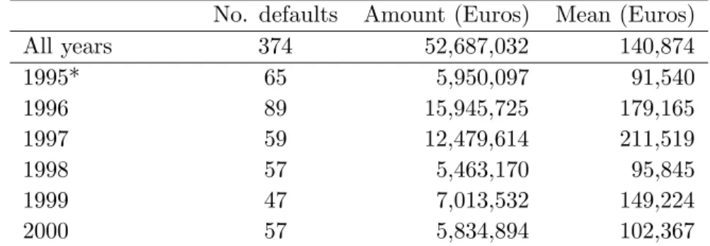
The dataset was provided by the largest private bank in Portugal, Banco Comercial Portuguˆes. The sample contains 374 loans granted to small and medium size enterprises (SMEs) that defaulted between June 1995 and December 2000. All firms have turnovers greater that 2.5 million Euros. Table 1 shows information on the number of observations, loan amount and mean loan amount in each year. The number of defaults in 1995 and 1996 is somewhat higher than in the remaining years, although there was no significant recession in the period covered by the data. About half of the observations correspond to debt amounts of less than 50,000 Euros.
No. defaults Amount (Euros) Mean (Euros)
All years 374 52,687,032 140,874 1995* 65 5,950,097 91,540 1996 89 15,945,725 179,165 1997 59 12,479,614 211,519 1998 57 5,463,170 95,845 1999 47 7,013,532 149,224 2000 57 5,834,894 102,367 * second semester
Table 1: Number of defaulted loans, debt amount and mean debt amount, organized by year of default.
Borrowing firms are classified into four broad groups according to their business sector: (i) real (activities with real assets, such as land, equipment or real estate), (ii) manufac-turing, (iii) trade and (iv) services. To each individual loan is attributed a rating by the bank’s internal rating system. The rating reflects not only the probability of default of the loan but also the guarantees and collateral that support the operation. There are seven classes of rating: A (the best), B, C1, C2, C3, D and E (the worst). These alpha-numeric rating notches were transformed into numeric values by an ordinal encoding that assigns the value 1 to rating A, the value 2 to rating B, and so on. Nearly half of the loans had no rating attributed. In order to avoid the exclusion of loans with missing rating class, which would reduce significantly the number of available observations, a surrogate rating equal to the mean value of the ratings in the sample was given to unrated loans. Fifty eight per cent of the loans are covered by personal guarantees. These are written promises that grant to the bank the right to collect the debt against personal assets pledged by the obligor. Fifteen per cent of the loans are covered by several varieties of collateral. These include real estate, inventories, bank deposits, bonds and stocks. Thirty six per cent of the loans are not covered by personal guarantees or any form of collateral. The loans are also characterized by the contractual lending rate, the age of the borrowing firm and the number of years of relationship with the bank. The mean age of the firms is 17 years while the mean age of relationship with the bank is 6 years.
1
Two methodologies are usually found in the literature to calculate recovery rates. The first methodology considers the market price of the loan at the time of emergence from default. This approach is common in studies concerning recoveries on corporate bond defaults, but it is also employed in studies of bank loan recoveries when a secondary mar-ket for defaulted loans is available (e.g., Gupton et al. (2000)) The second methodology considers the discounted value of cash or securities recovered during the bankruptcy reso-lution process. These approaches may give considerably different estimated recovery rates. The discrepancies may be attributed to substantial risk premia demanded by the market of defaulted loans (Carty et al., 1998). Because there were no secondary market prices available for the bank loans studied here, recovery rates were estimated using cash-flows recovered after default. The database includes the monthly history of cash-flows received by the bank after the loans became non-performing. These cash-flows include incoming payments due to the realization of collateral. For some loans, those of June 1995, a long recovery history of 66 months is available. As the default date approaches the end of year 2000, the recovery history is shortened. The discount rate that is used to compute the present value of the post-default cash-flows is the loan-specific contractual lending rate. While this rate may not capture the total risk of the firm after default, a substantial part of the total recovery is collected in the first months of the work-out process and, therefore, calculated recoveries should not change dramatically with the discount rate. Recoveries were computed using Altman (1989) mortality based approach.2
The costs of the resolution process are not considered in the calculation of the recovery rates.3
Figure 1 shows the distribution of cumulative recovery rates for horizons of 12, 24, 36 and 48 months after the default event. The distributions are bimodal with many observations with low recovery and many with complete recovery. Bimodal distributions of bank loan recoveries are also found in Asarnow and Edwards (1995), Felsovalyi and Hurt (1998), Franks et al. (2004), Araten et al. (2004) and Caselli et al. (2008). The frequency of complete recoveries increases with the recovery horizon as more cash-flows are collected in the work-out process.
Table 2 provides some basic statistics of the cumulative recovery rate distributions. The first row shows the number of loans that have a complete recovery history available for the respective horizon. For a recovery horizon of 12 months all defaults that occurred in the last available year (i.e., year 2000) are not considered, and likewise for other horizons. As expected the mean recovery rate increases with the recovery horizon as more cash-flows are collected. The median recovery rate exhibits a large jump when the horizon increases from 12 months to 24 months, as a consequence of the large increment in the number of near complete recoveries and the large reduction in the number of low recoveries. Figure 1 and Table 2 show that there are no substantial differences between the recovery distributions for horizons of 24, 36 and 48 months. This is a consequence of a marginal recovery rate that decreases rapidly with time after default. One can also observe a reduction in the standard deviation of the recovery distributions as the horizon increases.
2
For details, including a numerical example, see Dermine and Neto de Carvalho (2006).
3
Dermine and Neto de Carvalho (2006) estimate that the average cost of internal resolution processes is 1.2% of the amount received. When the contentious department has to rely on external lawyers, the average recovery cost increases to 10.4%.
Figure 1: Distribution of the cumulative recovery rate for recovery horizons of 12, 24, 36 and 48 months after the default event.
12 months 24 months 36 months 48 months
Number of observations 317 270 213 154
Mean 0.503 0.646 0.694 0.714
Median 0.493 0.907 0.946 0.950
Standard deviation 0.437 0.411 0.385 0.375
Table 2: Number of observations, mean, median and standard deviation of the recovery rate distributions for recovery horizons of 12, 24, 36 and 48 months.
3
Fractional response regression
In this section, a parametric regression of the recovery rate, r, as a function of the loan and firm characteristics, xi, i = 1, ..., k, is attempted. As Figure 1 shows, the recovery
rate is restricted to the interval between 0 and 1. Due to the bounded nature of the dependent variable one cannot implement an ordinary least squares (OLS) regression,
E(r|x) =β0+β1x1+...+βkxk =xβ, (1)
since the predicted values from the OLS regression can never be guaranteed to lie in the unit interval. An alternative specification to equation (1) is
where G(.) satisfies 0 < G(z) < 1 for all z ∈ R. This condition guarantees that the predicted recovery rates lie in the unit interval. The most common functional forms for G(.) are the cumulative normal distribution, the logistic function,
G(xβ) = 1
1 + exp(−xβ), (3)
and the log-log function,
G(xβ) = exp(−exp(−xβ)). (4) The non-linear estimation procedure consists of the maximization of the Bernoulli log-likelihood function (Papke and Wooldridge, 1996),
li(β)ˆ ≡rilog[G(xiβ)] + (1ˆ −ri) log[1−G(xiβ)].ˆ (5)
The quasi-maximum likelihood estimator of β is consistent and asymptotically normal regardless of the distribution of the recovery rate ri conditional on xi (Gourieroux et al.,
1984).
Table 3 reports the model coefficients that were obtained for recovery horizons of 12, 24, 36 and 48 months after the default event. The p-values are shown in parenthesis. These results were obtained with the log-log functional form, but the conclusions for the logistic functional form are similar. The last row in Table 3 shows that the Wald test for the null hypothesis that the set of coefficients are jointly zero is strongly rejected. Given the non-linearity of the functions G(xβ), the partial effects of the explanatory variables on recovery rates are not constant. The partial effect of variable xj on the recovery rate
is given by:
∂E(r|x) ∂xj
= dG(xβ)
d(xβ) βj. (6)
Because G(xβ) is strictly monotonic the sign of the coefficient gives the direction of the partial effects.
The first remark is that the size of the loan has a statistically significant negative effect on recovery rates at all recovery horizons. This behavior of the recovery rates is also observed in the study of Felsovalyi and Hurt (1998). On the other hand, Asarnow and Edwards (1995), Carty and Lieberman (1996) and Franks et al. (2004) report no relation between recovery rates and the size of loan. Dermine and Neto de Carvalho (2006) suggest that the negative effect of the debt amount on recovery rates may be explained by the reluctance of banks to foreclose large loans, hoping to preserve the option value of a future relationship. The collateral dummy variable is statistically significant at 10% level for recovery horizons of 24, 36 and 48 months and, as expected, has a positive impact on recoveries due to the realization of collateral. On the other hand, the personal guarantees dummy variable has a statistically significant negative impact on recoveries for 12 and 24 months horizons, at 10% level. A possible explanation for this counterintuitive result is that low risk clients may be exempt from providing personal guarantees. For 12 and 24 months horizons, the business sector dummies are not significant, suggesting that the regressions fail to capture industry-level variability. For 36 and 48 months horizons, the Trade sector dummy is significant and negative, suggesting that recoveries in this sector are lower than those in the base case (the Real sector). A similar observation can be made
Variable 12 months 24 months 36 months 48 months Constant 1.138 (0.019) 1.625 (0.008) 2.289 (0.004) 2.355 (0.049) Loan size -0.570 (0.001) -0.757 (0.000) -0.828 (0.000) -0.813 (0.000) Collateral 0.198 (0.368) 0.627 (0.054) 0.703 (0.072) 1.700 (0.000) Personal guarantees -0.275 (0.081) -0.401 (0.042) -0.227 (0.335) -0.460 (0.121) Manufacturing sector -0.186 (0.416) -0.274 (0.305) -0.314 (0.383) -1.159 (0.019) Trade sector -0.157 (0.443) -0.200 (0.413) -0.609 (0.048) -1.201 (0.008) Services sector -0.197 (0.417) 0.039 (0.902) 0.118 (0.783) -0.412 (0.486) Lending rate 0.020 (0.226) -0.006 (0.779) -0.023 (0.431) -0.021 (0.612) Age of firm 0.001 (0.055) 0.001 (0.054) 0.001 (0.075) 0.001 (0.063) Rating -0.234 (0.001) -0.212 (0.014) -0.176 (0.098) -0.068 (0.710) Years of relationship 0.003 (0.198) 0.007 (0.017) 0.003 (0.394) 0.006 (0.207) Wald test (χ2) 54.1 (0.000) 103.6 (0.000) 117.9 (0.000) 115.1 (0.000)
Table 3: Model coefficients given by a fractional response regression for recovery horizons of 12, 24, 36 and 48 months after default. The p-values are shown in parenthesis. A log-log functional form was used.
for the Manufacturing sector and for a recovery horizon of 48 months. The contractual lending rate is not significant. The age of firm has a statistically significant positive effect on recovery rates at 10% level, across all horizons. This result suggests that older firms exhibit better recoveries. The rating is significant for 12, 24 and 36 months recovery horizons at 10% level. The sign of the coefficients is in agreement with the expected direction of the partial effect: poor creditworthiness results in lower recoveries. Finally, the age of the obligor’s relationship with the bank is only significant at 5% level for a 24 months recovery horizon.
4
Regression trees
Regression trees (Breiman et al., 1984) are nonparametric and nonlinear predictive models in which the original dataset is recursively partitioned into smaller mutually exclusive subsets using a greedy search algorithm. A regression tree model is represented by a series of logical if-then conditions. Suppose one has a set of observations (i.e., bank loans) described by several attributes and a target variable (i.e., recoveries). The algorithm begins with a root node containing all observations. Then it searches over all possible binary splits of all available attributes for the one which will minimize the intra-subset variation of the target variable in the newly created daughter nodes. That is, in each daughter node the target variable will be more homogeneous than in the parent node. This procedure is repeated recursively for new daughter nodes until no further reduction in the variation of the target variable is achievable. Unsplit terminal nodes are denoted by ‘leaves’ and are depicted by rectangles in the tree graphs shown below. The decrease in the variance of the target variable is measured by the ‘standard deviation reduction’,
SDR=σ(T)− m(T1)
m(T)σ(T1)−
m(T2)
where T is the set of observations in the parent node and T1 and T2 are the set of
observations in the daughter nodes that result from splitting the parent node according to the optimal attribute. The operators m(.) and σ(.) represent the mean and standard deviation of the target variable in the set. Starting from the root node, all observations flow down the tree and terminate their path in a leaf. The predictions are given by the average value of the target variable for the set of observations in each leaf. Because the predictions are given by averages of recovery values, they are inevitably bounded between 0 and 1, and, therefore, regression trees are particularly appropriate for modeling recovery rates.
Very frequently the resulting trees are quite large and will overfit the data, giving good predictive accuracies on the data employed in the growth process but poor accuracies on new data. Improved accuracies on unobserved data can be obtained by ‘pruning’ the tree after the basic growth process. The pruning procedure examines each node of the tree, starting at the bottom. An estimate of the expected variance of the target variable that will be experienced at each node for unobserved data is evaluated. If the variance of a subtree is greater than the variance of the parent node, then the parent node is pruned to a leaf. This process is repeated until pruning no longer improves the error.4
Regression trees are not affected by the presence of outliers, since these are isolated into a node and have no further effect on the splitting. Furthermore, the resulting trees are invariant under monotone transformation of the explanatory variables. Regression trees are particularly suited to higher dimensionality problems and, as shown below, they can produce accurate results using only a few important explanatory variables.
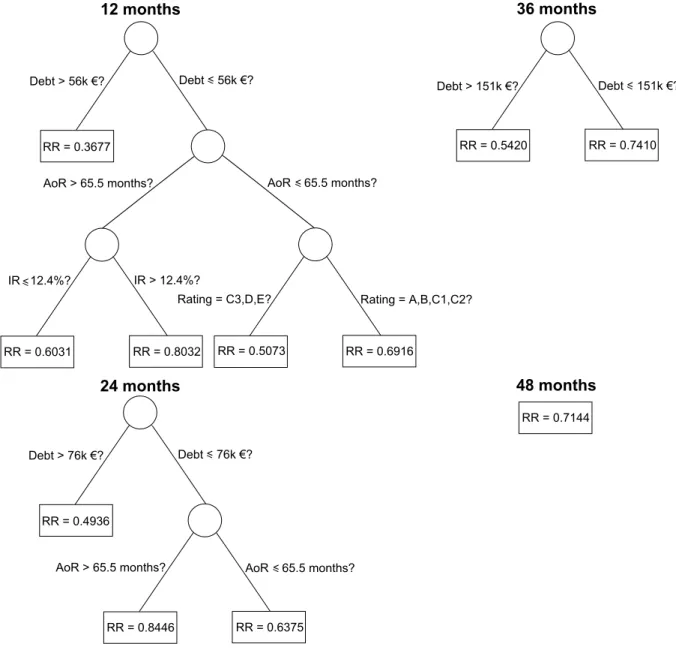
The interpretation of regression trees is clear and easily understood. In the upper left corner of Figure 2 one can find the regression tree obtained for the recovery horizon of 12 months after default. This tree may be interpreted in the following way. First, it is asked if the loan size (Debt) is greater than 56,000 Euros. If the answer is ‘yes’, then the expected recovery rate is 0.3677 and the branch ends there. If the answer is ‘no’ it is subsequently asked if the age of the client’s relationship with the bank (AoR) is smaller than 65.5 months. If the answer is ‘yes’ and the rating of the operation is A, B, C1 or C2, then the expected recovery is 0.6916; if the rating is C3, D or E then the expected recovery is 0.5073. If, on the other hand, the age of the client’s relationship with the bank is greater than 65.5 months and the contractual lending rate is smaller than 12.4% then the expected recovery is 0.6031; if the lending rate is greater than 12.4% then the expected recovery is 0.8032.
Therefore, the following conclusions may be drawn. Smaller recoveries are expected for larger loan sizes since the recovery in the branch corresponding to loan sizes greater than 56,000 Euros (0.3677) is smaller than any of the remaining predicted recoveries present in the tree. This observation corroborates the result given by the fractional response regression. For smaller loan sizes, one may expect greater recoveries if the age of the client’s relationship with the bank is greater (0.8032 and 0.6031 for AoR > 65.5 months versus 0.6916 and 0.5073 for AoR ≤65.5 months). If the loan size is small and the age of relationship is large, the recovery will be larger if the contractual lending rate is higher. On the other hand, if the loan size is small and the age of relationship is also small the recovery
4
Technical details of the specific implementation of regression trees employed in this work can be found in Wang and Witten (1996).
Figure 2: Regression trees for recovery horizons of 12, 24, 36 and 48 months. will be larger if the operation rating is good. Note that regression trees can capture effects on recovery rates due to explanatory variables that were statistically insignificant in the fractional response regression, such as the contractual lending rate and the age of the client’s relationship with the bank. Furthermore, a regression tree is conceptually similar to a look-up table, since the predictions are given by average recoveries. However, in a regression tree model the cells are defined by the data itself with no intervention by the analyst.
The tree for a recovery horizon of 24 months after default is simpler and is show in the lower left corner of Figure 2. Again, larger debt sizes result in smaller recoveries, but the threshold value (76,000 Euros) is larger than the respective value in the 12 months recovery horizon tree. If the loan size is smaller than 76,000 Euros, than the expected recovery is higher if the age of the client’s relationship is greater than 65.5 months. The tree for a 36
months recovery horizon is shown in the upper right corner of Figure 2 and is composed of a single binary split. Once more, larger debt sizes result in smaller predicted recoveries. For a recovery horizon of 48 months the tree is reduced to the root node and the expected recovery is equal to the mean value of the recoveries in the sample. That is, the tree model is equivalent to a model in which the expected recovery is equal to the historical average. As the recovery horizon increases, tree structures gets simpler as a consequence of the decreasing number of observations and the increasing homogeneity of the recovery rates. As shown below, the predictive accuracy of regression trees with respect to the fractional response regression is also deteriorated for longer recovery horizons.
5
Out-of-sample predictive accuracy
The expected predictive accuracy of the developed models on new data is assessed using two performance measures: the root mean squared error (RMSE) and the mean absolute error (MAE). The RMSE is defined as
RMSE = s 1 n X i (ri−rˆi)2, (8)
where ri and ˆri are the actual and predicted recovery rates on loani, respectively, and n is the number of loans in the sample. The MAE is defined as
MAE = 1 n
X
i
|ri−rˆi|. (9)
Models with lower RMSE and MAE have smaller differences between the actual and predicted recoveries and predict actual recoveries more accurately. The RMSE gives higher weights to large forecasting errors and, therefore, the RMSE is more helpful when these are particularly undesirable.
Because the developed models may overfit the data, resulting in over-optimistic es-timates of the predictive accuracy, the RMSE and MAE must be assessed on a sample which is independent from that used in building the models. A common technique to avoid over-fitting the data consists of randomly dividing the data sample in two sets: one set is used to fit the model and the other set is used to test its accuracy. This approach wastes valuable data since a reasonably large test sample is needed to evaluate accurately the prediction error. In order to develop models with a large fraction of the available data and evaluate the predictive accuracy with the complete dataset a 10-fold cross-validation was implemented. In this approach, the original sample is partitioned into 10 subsamples of approximately equal size. Of the 10 subsamples, a single subsample is retained for testing the model and the remaining 9 subsamples are used for building the model. The cross-validation process is repeated 10 times, with each of the 10 subsamples used exactly once as test data. The results from the 10 folds are then combined to produce a single estimate of the prediction error using the complete dataset. To reduce variability, the cross-validation procedure was repeated 1,000 times using different randomly generated 10-fold partitions.
12 months 24 months 36 months 48 months
Model RMSE MAE RMSE MAE RMSE MAE RMSE MAE
Log-log 0.432 0.398 0.403 0.357 0.383 0.328 0.365 0.296 (0.002) (0.002) (0.002) (0.002) (0.003) (0.003) (0.004) (0.004) Logistic 0.430 0.396 0.403 0.355 0.382 0.327 0.365 0.296 (0.002) (0.002) (0.002) (0.002) (0.003) (0.002) (0.004) (0.004) Trees 0.407 0.363 0.388 0.338 0.387 0.337 0.374 0.324 (0.004) (0.004) (0.004) (0.004) (0.004) (0.004) − − Historical 0.437 0.416 0.410 0.380 0.384 0.344 0.374 0.324
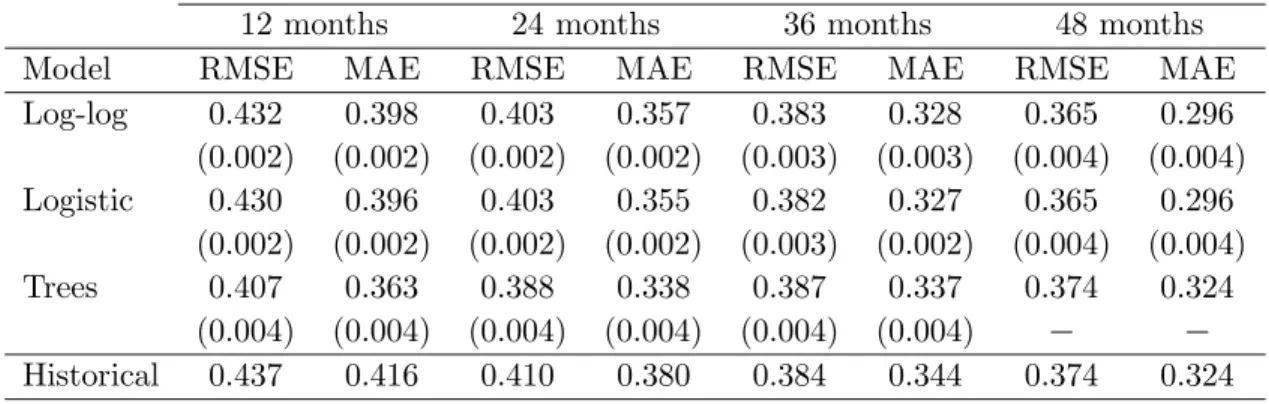
Table 4: Root mean squared errors (RMSE) and mean absolute errors (MAE) of the recovery rate estimates given by 10-fold cross-validation for recovery horizons of 12, 24, 36 and 48 months, and for the fractional log-log regression, the fractional logistic regression, the regression tree and the model in which the predicted recovery is equal to the historical average. These numbers refer to average values over 1,000 random 10-fold partitions. The standard deviations are shown in parenthesis.
Table 4 shows the average RMSE and MAE, over 1,000 rounds, of the recovery rate predictions given by the fractional response regressions and the regression trees. The results for both the logistic and log-log functional forms of the fractional response regres-sion are reported. For comparison, the last row of Table 4 shows the performance of a model in which predicted recovery rates are obtained from simple historical averages. The standard deviations are shown in parenthesis.
It can be observed that the logistic and log-log functional forms do not exhibit sub-stantial differences in forecasting performance. Also, the performance of the fractional response regressions is slightly superior to that of the model based on historical averages, across all recovery horizons. For recovery horizons of 12 and 24 months, the predictive ac-curacy of regression trees is clearly better than that of the fractional response regressions and the historical averages. However, the performance of regression trees is degraded for larger horizons and the best model is the fractional response regression. For a recovery horizon of 36 months, the tree with a single binary split fails to outperform the model based on historical averages. Of course, for a recovery horizon of 48 months the regression tree is equivalent to the model based on historical averages, since the tree is reduced to a single leaf containing all observations.
6
Out-of-time predictive accuracy
In Sections 3 and 4, the complete dataset was employed in the development of the models and in Section 5 the expected forecasting accuracy of these models on new data was evaluated via 10-fold cross-validation. However, this technique precludes the assessment of model accuracies over different periods of time. This section reports the forecasting accuracy of the models on an out-of-time sample. In this approach, the models are fit using data from a time period and the predictive accuracy is measured on a subsequent period. Given the constraint in the number of observations, only recovery rates with 12 months recovery horizon were considered. The forecasting accuracy in a given year was
evaluated using models that were developed using all data available before that year. First, the models were fit using loans that defaulted in years 1995 and 1996 and the predictive accuracy was measured on defaults that occurred in 1997. Then, the models were developed using defaults from years 1995, 1996 and 1997, and the accuracy was evaluated on defaults that occurred in 1998. Finally, the models were fit using loans that defaulted in years 1995, 1996, 1997 and 1998 and the accuracy was measured on defaults that occurred in 1999.
Table 5 reports the RMSE and MAE of predicted recovery rates in the out-of-time samples, given by the fractional response regressions and the regression tree.5
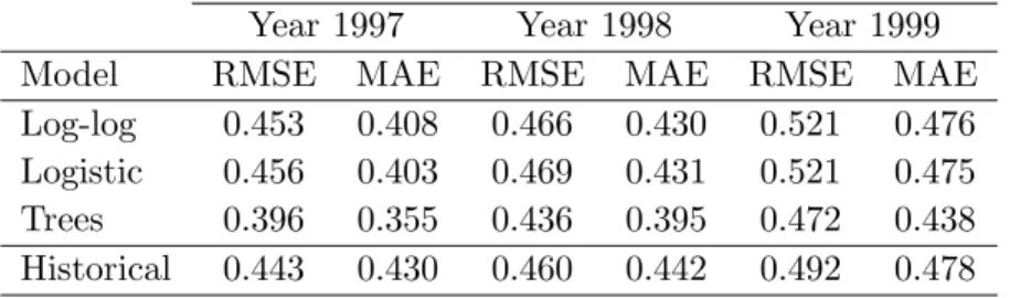
The results for the benchmark model in which the predicted recoveries are given by the average recovery in the previous period are also reported. The fractional response regressions give poor results and do not outperform the historical averages in terms of RMSE. In terms of MAE, the forecasting accuracies are better than those of the benchmark. Again, the logistic and log-log functional forms do not exhibit substantial differences in terms of accuracy. The predictive accuracy of the regression tree is better than that of the fractional response regressions and the historical averages across all years, in terms of both RMSE and MAE.
Year 1997 Year 1998 Year 1999
Model RMSE MAE RMSE MAE RMSE MAE
Log-log 0.453 0.408 0.466 0.430 0.521 0.476 Logistic 0.456 0.403 0.469 0.431 0.521 0.475 Trees 0.396 0.355 0.436 0.395 0.472 0.438 Historical 0.443 0.430 0.460 0.442 0.492 0.478
Table 5: Root mean squared errors (RMSE) and mean absolute errors (MAE) of the predicted recovery rates in out-of-time samples for a recovery horizon of 12 months, and for the fractional log-log regression, the fractional logistic regression, the regression tree and the model in which the predicted recovery is equal to the historical average.
7
Conclusions
This study evaluated the performance of a parametric fractional response regression and a nonparametric regression tree model to forecast bank loan credit losses. Recovery rate models for several recovery horizons were implemented and analyzed. The regression tree models captured effects on recovery rates due to explanatory variables that were statistically insignificant in the fractional response regression. The forecasting accuracy of these models was evaluated using two different approaches: an out-of-sample estimation using the complete dataset with the help of a 10-fold cross-validation, and an out-of-time estimation in which the models are fit using defaults from one period and the accuracy is measured on defaults from the following year. The performance of the models was
5
benchmarked against predicted recoveries given by historical averages. When out-of-sample estimation was considered, the regression trees gave better results for shorter recovery horizons of 12 and 24 months, while the fractional response regression gave better results for longer horizons. The regression tree gave the best results for out-of-time estimation of the predictive accuracies. On the other hand, the fractional response regression did not outperform the model based on historical averages in terms of RMSE. The reader should note that this study is based on data from an individual bank in a single country and, therefore, these results will certainly capture some of the bank’s intrinsic characteristics. In fact, Franks et al. (2004) reported that recovery rate distri-butions exhibit not only country-based differences, reflecting different insolvency regimes, but vary as well across banks within the same country. Nevertheless, the results shown here capture several empirical regularities found in previous studies on recovery rates. The models tested here are parsimonious, give results that are easily interpretable and are readily implemented. In particular, the results suggest that regression trees are an interesting alternative to the parametric models commonly employed in empirical studies on recovery rates.
Acknowledgments
I am very grateful to Cristina Neto de Carvalho for supplying the data for this study and for her invaluable help in the analysis. I would also like to thank Jo˜ao Santos Silva for his helpful comments and suggestions. This study was supported by a grant from the Funda¸c˜ao para a Ciˆencia e Tecnologia.
References
V. V. Acharya, S. T. Bharath, and A. Srinivasan. Does industry-wide distress affect defaulted loans? evidence from creditor recoveries. Journal of Financial Economics, 85:787–821, 2007.
E. I. Altman. Default recovery rates and LGD in credit risk modeling and practice: An updated review of the literature and empirical evidence. Working paper, Stern School of Business, New York University, 2006.
E. I. Altman. Measuring corporate bond mortality and performance. Journal of Finance, 44(4):909–922, 1989.
M. Araten, M. Jacobs Jr., and P. Varshney. Measuring LGD on commercial loans: An 18-year internal study. The RMA journal, 4:96–103, 2004.
E. Asarnow and D. Edwards. Measuring loss on defaulted bank loans: A 24-year study. Journal of Commercial Lending, 77(7):11–23, 1995.
Basel Committee on Banking Supervision. International convergence of capital measure-ment and capital standards. Technical report, BIS, 2006.
T. Bellotti and J. Crook. Modelling and predicting loss given default for credit cards. Working paper, Quantitative Financial Risk Management Centre, 2007.
L. Breiman, J. H. Friedman, R. A. Olshen, and C. J. Stone. Classification and regression trees. Wadworth International Group, Belmont, California, 1984.
L. V. Carty and D. T. Hamilton. Debt recoveries for corporate bankruptcies. Moody’s Investors Service, 1999.
L. V. Carty and D. Lieberman. Defaulted bank loan recoveries. Moody’s Investors Service, 1996.
L. V. Carty, D. T. Hamilton, S. C. Keenan, A. Moss, M. Mulvaney, T. Marshella, and M. G. Subhas. Bankrupt bank loan recoveries. Moody’s Investors Service, 1998. S. Caselli, S. Gatti, and F. Querci. The sensitivity of the loss given default rate to
systematic risk: New empirical evidence on bank loans. Journal of Financial Services Research, 34(1):1–34, 2008.
J. Dermine and C. Neto de Carvalho. Bank loan losses-given-default: A case study. Journal of Banking and Finance, 30:1291–1243, 2006.
A. Felsovalyi and L. Hurt. Measuring loss on latin american defaulted bank loans: A 27-year study of 27 countries. Journal of Lending and Credit Risk Management, 80: 41–46, 1998.
J. Franks, A. de Servigny, and S. Davydenko. A comparative analysis of the recovery pro-cess and recovery rates for private companies in the UK, france and germany. Standard and Poor’s report, 2004.
C. Gourieroux, A. Monfort, and A. Trognon. Pseudo-maximum likelihood methods: the-ory. Econometrica, 52:681–700, 1984.
J. Grunert and M. Weber. Recovery rates of commercial lending: Empirical evidence for german companies. Journal of Banking and Finance, 33:505–513, 2009.
G. M. Gupton and R. M. Stein. LossCalc V2: Dinamic prediction of LGD. Moody’s Investors Service, 2005.
G. M. Gupton, D. Gates, and L. V. Carty. Bank loan loss given default. Moody’s Investors Service, 2000.
S. O’Shea, S. Bonelli, and R. Grossman. Bank loan and bond recovery study; 1997-2000. Fitch IBCA, 2001.
L. E. Papke and J. M. Wooldridge. Econometric methods for fractional response variables with an application to 401(k) plan participation rates.Journal of Applied Econometrics, 11:619–632, 1996.
T. Schuermann. What do we know about loss given default. Working paper no. 04-01, Wharton Financial Institutions Center, 2004.
Y. Wang and I. H. Witten. Induction of model trees for predicting continuous classes. Working paper, Department of Computer Science, University of Waikato, 1996.