Handling Imbalanced Classes: Feature Based Variance Ranking Techniques for Classification

Feature Based Variance

Ranking Techniques for

Classification

Solomon Henry EBENUWA

A thesis submitted in partial fulfilment

of the requirements of the University

of East London for the degree of

Doctor of Philosophy

Architecture, Computing and Engineering (ACE),

University of East London

Dr Ameer Al-Nemrat

Senior Lecturer in Computer Science

School of Architecture, Computing and Engineering (ACE) University of East London,

Docklands Campus, 4-6 University Way, London E16 2RD

Dr Saeed Sharif

Senior Lecturer in Computer Science

School of Architecture, Computing and Engineering (ACE) University of East London,

Docklands Campus, 4-6 University Way, London E16 2RD

To obtain good predictions in the presence of imbalance classes has posed significant challenges in the data science community. Imbalanced classed data is a term used to describe a situation where there are unequal number of classes or groups in datasets. In most real-life datasets one of the classes are always higher in number than others and is called the majority class, while the smaller classes are called the minority class. During classifications even with very high accuracy, the classified minority groups are usually very small when compared to the total number of minority in the datasets and more often than not, the minority classes are what is being sought. This work is specifically concern with providing techniques to improve classifications performance by eliminating or reducing negative effects of class imbalance. Real-life datasets have been found to contain different types of error in combination with class imbalance. While these errors are easily corrected, but the solutions to class imbalance have remained elusive.

Previously, machine learning (ML) technique has been used to solve the problems of class imbalanced. There are notable shortcomings that have been identified while using this technique. Mostly, it involve fine-tuning and changing parameters of the algorithms and this process is not standardised because of countless numbers of algo-rithms and parameters. In general, the results obtained from these unstandardised

(ML)technique are very inconsistent and cannot be replicated with similar datasets and algorithms

We present a novel technique for dealing with imbalanced classes called variance ranking features selection, that enables machine learning algorithms to classify more of minority classes during classification, hence reducing the negative effects of class imbalance. Our approaches utilised the intrinsic property of the datasets called the variance. As the variance is one of the measures of central tendency of the data items concentration within the datasets vector space. We demonstrated the selections of features at different level of performance threshold thereby providing an opportunity for performance and feature significance to be assessed and correlated at different levels of prediction. In the evaluations we compared our features selections with some of the best known features selections techniques using proximity distance comparison techniques and verify all the results with different datasets, both binary and multi classed with varying degree of class imbalance. In all the experiments, the

This work is dedicated to those who had to take the brave journey alone. It was cold, lonely and bitter, there was no person nor place to get help. The pains, anxiety and despondence we had to bear, the endless wobbling and falling, the wiping out of my resources and stagnation of every aspects of my existence while waiting for the journey to end. There were days when it seems is not going to end, on hindsight I wondered what kept me going. Some day, perhaps it may be worth all the toiling.

I Solomon Henry EBENUWA, Solemnly declare that the work in this thesis are my and that every effort have been made to acknowledge all the academic papers, Journals, book and other material used in accordance to academic best practises by providing appropriate reference. I further state that some part of this thesis have been and will be publish in academic papers, Journals, book and other materials for the purpose of advancing knowledge and information.

This research journey would have been impossible if not for the contributions of some notable individuals, I used this juncture to acknowledge their contributions and say a big thank you to them.

First and formost are my able supervisory teams being led by the person of Dr Ameer Nemrat my Director of Studies (DOS) and Dr Saeed Shareef (Supervisor), I would also note the contributions of my first supervisor that started the Journey with me Dr Abdul Tawil, I will remain grateful for all the support, encouragement, endless meetings and corrections that you men provided me with. On many occasions I had wanted to dropout but each time I meet with either of you my interest is reinvigorated and I have a new reason to fight on. You gentlemen provided me an invaluable advise, insight and strength without which this P.hD journey would not have been possible , once again I say ”THANK YOU” and ”Doff My Hat”.

I will not forget the contributions of the following colleagues and friends; notably the person of Dr Kennedy Isibor Ihianle, who specifically introduced me to many skills I had to acquire for a successful Ph.d Journey and insights into Journal publications without which my success today may not have been realistic.

I use this time to recognize the contributions of my senior sister Ms Uche Stella EBENUWA and her daughter Jennifer, there were times when it was only we three that was around each other, there were darkness and hopelessness everywhere how we were able to cope and persevere is still a mystery to me; I really hope that we could one day seat and reminisce.

Finally, I give thanks to God the creator or what ever that is up there watching over me, I believe without any iota of doubt that ”Something or Someone” is watching over me! On many occasion I have face an extreme situation that made me think that I am a ”lost cause” , the situation was hopeless, but some how I manage to survive, begin again and even prosper. Its just cannot be that is due to my effort because my efforts alone would not have been enough to extricate me from the quagmires that have dug my life ever since, to this I say Thank YOU GOD!. Let me recognise the contribution of certain people earlier in my life Mr Osadebe, Mr Franklin Eghomien; Oh my God! I remember my time at UNIBEN if not for you two, it would have been worst. I am also acknowledging the contributions of all those I did not mention their names here because of space, particularly the people

desire. For all my former friends that I have fallen apart with, I still say thank you because as at the time we were friends you contributed in making life bearable. I thank those that will have the patience to read this research work and I say to them, may it give you as much pleasure and excitements as it has given me during the research journey and also remember that a research work is not suppose to be a ”finish product” rather an opening to more knowledge questions and that lead to more questions for continuity and advancement of knowledge. For this I extend my thanks to those earlier researcher that their work is in the public domain for affording me the opportunity to read their work and hope that some day this work will also join them in the same public space.

List of Figures xii

List of Tables xvi

Glossary xx

1 Introduction 2

1.1 Problems with real life data sets . . . 3

1.1.1 Imbalanced class . . . 3

1.1.2 Data structuralization . . . 5

1.1.3 Dirty data . . . 5

1.1.4 Cleaning by data transformation . . . 6

1.1.5 Identifying outliers and noise . . . 6

1.1.6 High dimensionality. . . 8 1.2 Motivation . . . 9 1.3 Aims . . . 10 1.4 Contributions . . . 11 1.4.1 Terms Definitions . . . 12 1.5 Research Methodology . . . 12 1.5.1 List of Publication . . . 14

1.5.2 Summary of Thesis Report Layout . . . 15

2 Literature Review 17 2.1 Overview of imbalance data . . . 17

2.2 Techniques for handling imbalance class distribution. . . 19

2.2.1 Overview of machine learning algorithm . . . 20

2.2.2 Variance Techniques For Handling imbalanced classed data . . 21

2.2.3 Algorithm Techniques for imbalanced classed data . . . 22

2.2.4 Cost-Sensitive method . . . 28

2.2.5 Ensemble Methods . . . 31

2.2.6 Sampling based Methods . . . 32

2.2.7 The Attribute/Feature Selection Approaches to imbalanced dataset. . . 35

2.2.8 A Case for Hybrid Approach to Imbalanced classed Problems 37

2.2.9 Researcher’s Further Development. . . 38

2.3 The Measurement Evaluation for Imbalanced dataset . . . 39

2.3.1 Measurement Evaluation for Binary classed data . . . 39

2.3.2 Measurement Evaluation for Multi-classed data (One-Versus-all and One -Versus-One). . . 40

2.3.3 The Receiver Operating Characteristics and Area Under the Curve . . . 42

2.3.4 Data acquisition and descriptions: . . . 44

2.3.5 General Data preparation and Techniques to Avoid Overfitting. 45 3 Variance Ranking Attribute Selection Technique 49 3.1 Proposed Method and Approach . . . 49

3.1.1 Variance and Variables Properties . . . 50

3.2 The Abstraction and High level Research Design: . . . 56

3.3 Experiment Design: . . . 57

3.3.1 Sampling and Splitting the data set . . . 57

3.3.2 Experiments for Variance Ranking Attribute Selection . . . . 58

4 Comparison of Variance Ranking With Other Attributes Selection 71 4.1 Introduction . . . 71

4.2 Comparison of Variance Ranking Attribute Selection (VR) Technique with the Benchmarks . . . 72

4.3 Calculating Similarities of (VR) (PC) and (IG) using Ranked Order Similarity-(ROS) . . . 82

4.3.1 Levenshtein Similarity . . . 84

4.4 Motivation and Deriving Rank Order Similarity-(ROS) . . . 86

4.4.1 Comparison of Rank Order Similarity with Levenshtein Simi-larity . . . 90

4.5 The Results of Comparing (VR),(PC) and (IG) using (ROS) technique 91 5 Validation 98 5.0.1 Validation of (VR) Technique for Binary Imbalance Dataset . 100 5.0.2 Decision Tree Experiments for Pima diabetes Data . . . 101

5.0.3 Logistic Regression Experiments for Pima diabetes data . . . 104

5.0.4 Support Vector Machine Experiments for Pima diabetes data. 106 5.0.5 Decision Tree Experiments for Wisconsin Breast cancer data . 109 5.0.6 Logistic Regression Experiments for Wisconsin Breast cancer data . . . 111

5.0.7 Support Vector Machine Experiments for Wisconsin Breast cancer data . . . 113

5.0.8 Validation of (VR) technique for Multiclassed Imbalance Data set . . . 115

5.0.9 Validation Experiments using the Glass data set results . . . 117

5.0.10 Logistic Regression Experiments for Glass data using One vs

All (class 1 as 1 and the others as class 0 ) see table . . . 118

5.0.11 Decision Tree Experiments for Glass data using One vs All

(class 1 as 1 and the others as class 0 ) see table 5.15 . . . 120

5.0.12 Support Vector Machine for Glass data using One vs All (class 1 as 1 others as class 0) see table 5.15 . . . 122

5.0.13 Conclusion. . . 124

5.0.14 Logistic Regression Experiments for Glass Data Using One Versus All (Class 3 as Class 1 and the Others as Class 0)see table 5.15 . . . 124

5.0.15 Validation Experiments using the Yeast data set results . . . 126

5.0.16 Decision Tree Experiments for Yeast Data Using One Versus All (Class ERL(5) as 1 and the others as class 0 (1479)) see Table 5.15 . . . 126

5.0.17 Logistic Regression Experiments for Yeast data using One vs

All (class ERL(5) as 1 others as class 0 (1479)) see Table 5.15 129

5.0.18 Decision Tree and Support Vector Machine Experiments for Yeast data using One vs All (class VAC (30) as class 1 others as class 0 (1454)) see table 5.15 . . . 131

5.0.19 Logistic Regression Experiments for Yeast data using One vs All (class VAC (30) as class 1 others as class 0 (1454)) see table 5.15 . . . 132

5.0.20 Conclusion. . . 134

5.1 Comparison of Variance Ranking with the Work of Others On

Imbal-anced classed Data . . . 134

5.1.1 Introduction . . . 134

5.1.2 New approaches to Imbalanced Data And Introduction To

Sampling . . . 136

5.1.3 Similarities and Differences between (VR), (SMOTE) and (ADASYN)136

5.1.4 Performance comparisons Between (VR), (SMOTE) and (ADASYN)

on Common data sets . . . 139

5.1.5 Experiment Set up . . . 139

5.1.6 Conclusion. . . 141

6 Summary Discussion and Conclusions 143

6.1 Summary Critique of Existing Algorithm and Sampling Approaches . 143

6.1.1 Critique of Existing Algorithm Techniques. . . 144

6.1.3 Summary of the Contributions of this Thesis . . . 144 6.2 Recommendations. . . 145 6.3 Limitations . . . 146 6.4 Future Work . . . 147 6.4.1 Final Summary . . . 148 A Appendix 150 Bibliography 164

1.1 Problems of Real-Life data sets . . . 3

1.2 Interquartile Range . . . 7

1.3 Box and Whiskers. . . 8

2.1 Imbalanced and Balance data . . . 18

2.2 Machine learning algorithm . . . 20

2.3 Basic SVM imbalanced data points . . . 24

2.4 Decision Tree . . . 26

2.5 Neural Network . . . 27

2.6 Neural Network output . . . 27

2.7 Value of K is 3 in the sample space . . . 30

2.8 Multi-classed to Binary decomposition-One vs All . . . 41

2.9 Multi-classed to Binary decomposition-One vs One . . . 41

2.10 ROC Curve . . . 43

2.11 The Area Under the ROC Curve . . . 44

2.12 Deducing AUC . . . 44

2.13 K-Fold Cross validation. . . 47

3.1 An Overview of the Proposed Method. . . 50

3.2 Standard Deviation for Single Variable Normal Distribution . . . 51

3.3 3D Glass data Scatter plot . . . 52

3.4 Algorithm flow chart for The Variance Ranking Attribute Selection . 54 3.5 Glass data contents proportion . . . 63

3.6 Yeast data contents proportion . . . 65

4.1 Presentation of Euclidean and Manhattan distance . . . 83

4.2 Cosine Similarity . . . 84

4.3 Ranked Order Similarity-ROS Percentage Weighting Calculation for α and β . . . 88

4.4 Comparative Similarity between ROS and LEV . . . 90

5.1 Accuracy vs Number of Attributes for Pima data using Decision Tree 103 5.2 Recall vs Number of Attributes for Pima data using Decision Tree . . 104

5.3 Accuracy vs Number of Attributes for Pima data using Logistic Re-gression . . . 105

5.4 Recall vs Number of Attributes for Pima data using Logistic Regression106

5.5 Accuracy vs Number of Attributes for Pima data using Support

Vec-tor Machine . . . 107

5.6 Recall vs Number of Attributes for Pima data using Support Vector

Machine . . . 108

5.7 Graph of DT Accuracy vs Numbers of Attributes for Wisconsin data

showing (P T P)Accuracy . . . 110

5.8 Graph of DT Recall vs Numbers of Attributes for Wisconsin data

showing (P T P)Recall . . . 111

5.9 Graph of LR Accuracy vs Numbers of Attributes for Wisconsin data

showing (P T P)Accuracy at the position 6 attributes . . . 112

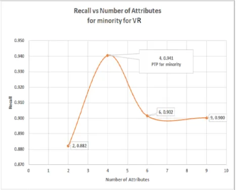
5.10 Graph of LR Recall vs Numbers of Attributes for Wisconsin data showing (P T P)minority at the position of 4 attributes . . . 113

5.11 Graph of SVM Accuracy vs Numbers of Attributes for Wisconsin data showing (P T P)Accuracy at the position of 4 attributes . . . 114

5.12 Graph of SVM Recall vs Numbers of Attributes for Wisconsin data showing (P T P)minority at the position of 4 attributes . . . 115

5.13 Graph of LR Accuracy vs Numbers of Attributes for Glass data Mi-nority class: Class 1 as 1 and the others as class 0, the (P T P)Accuracy

position. . . 119

5.14 Graph of LR Recall vs Numbers of Attributes for Glass data Minority class: Class 1 as 1 and the others as class 0, the (P T P)minority in

different position. . . 119

5.15 Graph of DT Accuracy vs Numbers of Attributes for Glass data Mi-nority class: Class 1 as 1 and the others as class 0 (P T P)Accuracy in

the 6 attribute position . . . 121

5.16 Graph of DT Recall vs Numbers of Attributes for Glass data Minority class: Class 1 as 1 and the others as class 0 (P T P)minority in the 4

attribute position . . . 121

5.17 Graph of SVM Accuracy vs Numbers of Attributes for Glass data Minority class: Class 1 as 1 and the others as class 0, (P T P)Accuracy

in the position of 4 attributes . . . 123

5.18 Graph of SVM Recall vs Numbers of Attributes for Glass data Mi-nority class: Class 1 as 1 and the others as class 0, (P T P)minority in

the position of 4 attributes . . . 123

5.19 Graph of LR Accuracy vs Numbers of Attributes for Glass data Mi-nority class: Class 3 as Class 1 and the others as class 0 (P T P)Accuracy

5.20 Graph of LR Recall vs Numbers of Attributes for Glass data Minority class: Class 3 as Class 1 and the others as class 0, (P T P)minority at

the position of 4 attributes . . . 125

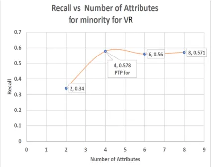
5.21 Extreme case of Ibalance of class ERL(5) as 1 others as class 0 (1479) 127 5.22 Graph of Accuracy vs Numbers of Attributes for Yeast class ERL(5) as class 1 and the others as class0(1479) for DT minority showing (P T P)Accuracy in both 8 and 4 attributes position . . . 128

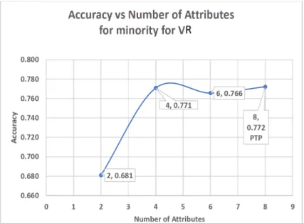
5.23 Graph of Recall vs Numbers of Attributes for Yeast class ERL(5) as 1 and the others as class0(1479) for DT minority showing (P T P)minority in the position of 4 attributes . . . 129

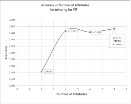
5.24 Graph of Accuracy vs Numbers of Attributes for Yeast class ERL(5) as class 1 and the others as class 0 (1479) for LR minority showing (P T P)Accuracy in the position of 2 attributes . . . 130

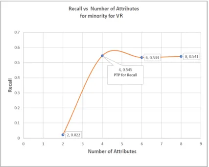
5.25 Graph of Recall vs Numbers of Attributes for Yeast class ERL(5) as class 1 and the others as class0(1479) for LR minority showing (P T P)minority in the position of 4 attributes . . . 131

5.26 Extreme case of Imbalance class VAC(30) as 1 others as class0 (1454).docx132 5.27 Graph of the Accuracy vs Numbers of Attributes for Yeast class VAC(30) as 1 others as class0(1454) for LR minority showing (P T P)Accuracy at the position of 8 attributes . . . 133

5.28 Graph of the Recall vs Numbers of Attributes for Yeast class VAC(30) as 1 others as class0(1454) for LR minority showing (P T P)minority at the position of 4 attributes . . . 134

5.29 3D Glass data Scatter plot . . . 137

5.30 3D Pima data Scatter plot . . . 138

5.31 3D Iris data Scatter plot . . . 138

5.32 Graph Evaluation Metric And Performance Comparison LR . . . 140

5.33 Graph Evaluation Metric And Performance Comparison DT . . . 141

5.34 Graph Evaluation Metric And Performance Comparison SVM . . . . 141

A.1 Weka Interface experiment for all features in Pima data using Decision Tree . . . 152

A.2 Weka Interface experiment for only two features in Pima data using Decision Tree . . . 152

A.3 Weka ROC for DT Wisconsin . . . 153

A.4 weka Glass class1 as1 other0 LR, for minority captured . . . 153

A.5 weka Glass class1 as1 other0 LR, for minority captured the ROC . . . 154

A.6 weka Glass class1 as1 other 0 DT-21 minority captured . . . 154

A.7 weka Glass class1 as 1 other 0 DT, 0 minority captured . . . 155

A.8 weka Glass class1 as1 other 0, DT 13 minority captured . . . 155

A.10 weka Glass class3 as1 other0 DT SVM, no minority captured . . . 156

A.11 Class Distribution Of Yeast Data . . . 157

A.12 weka Interface SVM for Wisconsin . . . 157

A.13 weka Interface SVM for Wisconsin-2 . . . 158

A.14 wekaYeastclassERL(5)as1othersasclass0(1479) for DT . . . 158

A.15 wekaYeastclassERL(5)as1othersasclass0(1479) the ROC for DT . . . . 159

A.16 wekaYeastclassERL(5)as1othersasclass0(1479) for DT capture 1 Mi-nority . . . 160

A.17 wekaYeastclassERL(5)as1othersasclass0(1479) the ROC Capture 1 for DT . . . 161

A.18 weka Interface for Yeast class ERL(5)as 1 others as class0(1479) for LR Capture all 5 minority . . . 162

A.19 weka Interface for Yeast class VAC(30)as 1 others as class0(1454) for DT Capture 0 minority . . . 162

A.20 weka Interface for Yeast class VAC(30)as 1 others as class0(1454) for ROC of DT Capture 0 minority . . . 163

A.21 weka Interface for Yeast class VAC(30)as 1 others as class0(1454) for SVM Capture 0 minority . . . 163

2.1 Cost Matrix Representation . . . 29

2.2 Common filter feature selection technique. . . 36

2.3 Literature review summary in Chapter 2 . . . 38

2.4 Confusion Matrix . . . 40

3.1 Variance Ranking attribute selection using Pima India data. . . 60

3.2 Variance Ranking attribute selection using Bupa data . . . 60

3.3 Variance Ranking attribute selection using Wisconsin Breast Cancer data . . . 61

3.4 Variance Ranking attribute selection using Cod-rna data . . . 61

3.5 Variance Ranking attribute selection using Iris data . . . 62

3.6 Glass data set details showing highly imbalance classes . . . 62

3.7 Glass data class relabel to One-vs-All . . . 64

3.8 Yeast data set details showing highly imbalance classes . . . 64

3.9 Yeast data class relabel to One-vs-All . . . 65

3.10 Experiment on Glass data . . . 66

3.11 Experiment on Yeast data . . . 68

3.12 Experiment on Yeast data continue . . . 69

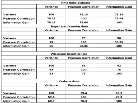
4.1 Comparison of Variance Ranking with PC and IG variable selection for Pima India diabetes data . . . 73

4.2 Comparison of Variance Ranking with PC and IG variable selection for Liver Disorder Bupa data. . . 73

4.3 Comparison of Variance Ranking with PC and IG variable selection for Wisconsin Breast cancer data . . . 73

4.4 Comparison of Variance Ranking with PC and IG variable selection for Cod-rna data . . . 74

4.5 Comparison of Variance Ranking with PC and IG variable selection for Iris data . . . 76

4.6 Comparison of Ranking significant with PC and IG variable selection for Glass data . . . 77

4.7 Comparison of Variance significant with PC and IG variable selection for Yeast data . . . 80

4.8 Comparison of Variance significant with PC and IG variable selection for Yeast data continue . . . 81

4.9 Levenshtein Process. . . 85

4.10 Comparing two string using Levenshtein Similarity techniques . . . . 86

4.11 Three Sets arranged and ranked in different order . . . 87

4.12 ROS Calculation between VR and PC for Sub-table ”ERL as class 1, others as class 0” in table 4.7 . . . 89

4.13 ROS Calculation between VR and PC for Sub-table ”ERL as class 1, others as class 0” in table 4.7 . . . 89

4.14 Comparison of Rank Order Similarity with Levenshtein Similarity . . 90

4.15 Comparison of (VR), (PC) and (IG) using the (ROS) technique for

Pima, Bupa, Wisconsin and Cor-rna data . . . 92

4.16 Comparison of (VR), (PC) and (IG) using the (ROS) technique for Iris data . . . 93

4.17 Comparison of (VR), (PC) and (IG) using the (ROS) technique for

Glass data . . . 93

4.18 Comparison of (VR), (PC) and (IG) using the (ROS) technique for

Glass data . . . 94

4.19 Comparison of (VR), (PC) and (IG) using the (ROS) technique for

Yeast data . . . 95

4.20 Comparison of (VR), (PC) and (IG) using the (ROS) technique for

Yeast data continue . . . 96

5.1 Comparison of (VR), (PC) and (PC) Attributes selection for Pima

India diabetes data . . . 102

5.2 Results of majority class for Pima data set for DT by (VR) feature

selection . . . 102

5.3 Results of minority class for Pima data set for DT by (VR) feature

selection . . . 103

5.4 Results of majority class for Pima data set for LR by (VR) feature

selection . . . 104

5.5 Results of minority class for Pima data set for LR by (VR) feature

selection . . . 105

5.6 Results of majority class for Pima data set for SVM by (VR) feature

selection . . . 106

5.7 Results of minority class for Pima data set for SVM by (VR) feature

selection . . . 107

5.8 Comparison of Variance significant with PC and IG variable selection

for Wisconsin Breast cancer data . . . 109

5.9 Results of majority class for Wisconsin data set for DT by (VR), (PC)

5.10 Results of minority class for Wisconsin data set for DT by (VR), (PC) and (IG) feature selection . . . 110

5.11 Results of majority class for Wisconsin data set for LR by (VR), (PC) and (IG) feature selection . . . 112

5.12 Results of minority class for Wisconsin data set for LR by (VR), (PC) and (IG) feature selection . . . 112

5.13 Results of majority class for Wisconsin data set for SVM by (VR),

(PC) and (IG) feature selection . . . 113

5.14 Results of minority class for Wisconsin data set for SVM by (VR),

(PC) and (IG) feature selection . . . 114

5.15 A section of 4.6 table for Glass data . . . 116

5.16 A section of 4.7 table for Yeast data. . . 116

5.17 Results of majority class for Glass data set for LR by (VR), (PC) and

(IG) feature selection for class 1 as 1 and the others other as class 0 . 118

5.18 Results of minority class for Glass data set for LR by (VR), (PC) and

(IG) feature selection for class 1 as 1 and the others as class 0 . . . . 118

5.19 Results of majority class for Glass data set for DT by (VR), (PC)

and (IG) feature selection for class 1 as 1 and the others as class 0 . . 120

5.20 Results of minority class for Glass data set for DT by (VR), (PC)

and (IG) feature selection for class 1 as 1 and the others as class 0 . . 120

5.21 Results of majority class for Glass data set for SVM by (VR), (PC) and (IG) feature selection for class 1 as 1 other as class 0 . . . 122

5.22 Results of minority class for Glass data set for SVM by (VR), (PC) and (IG) feature selection for class 1 as 1 other as class 0 . . . 122

5.23 Results of majority class for Glass data set for LR by (VR), (PC) and (IG) feature selection for class 3 as class 1 other as class 0 . . . 124

5.24 Results of minority class for Glass data set for LR by (VR), (PC) and (IG) feature selection for class 3 as class 1 other as class 0 . . . 124

5.25 Results of majority class for Yeast data set for DT by (VR), (PC) and (IG) feature selection for class ERL(5)as Class 1, Others(1479) as class0 . . . 127

5.26 Results of minority class for Yeast data set for DT by (VR), (PC) and (IG) feature selection for class ERL(5)as Class 1, Others(1479) as class 0. . . 128

5.27 Results of majority class for Yeast data set for LR by (VR), (PC) and (IG) feature selection for class ERL(5)as Class 1, Others(1479) as class0 . . . 129

5.28 Results of minority class for Yeast data set for LR by (VR), (PC) and (IG) feature selection for class ERL(5)as Class 1, and the others(1479) as class0 . . . 130

5.29 Results of majority class for Yeast data set for LR by (VR), (PC) and (IG) feature selection for class VAC(30)as Class 1, Others(1454) as class 0. . . 132

5.30 Results of minority class for Yeast data set for LR by (VR), (PC) and (IG) feature selection for class VAC(30)as Class 1, Others(1454) as class 0. . . 133

5.31 Evaluation Metric And Performance Comparison VR, SMOTE and

ADASYN . . . 140

A.1 Data used in the experiment continue . . . 150

(F Pmaj) False Positive Majority xix, 99, 117 (F Pmin) False Positive Minority xix, 99, 117 (T Pmaj) True Positive Majority xix, 99, 117 (T Pmin) True Positive Minority xix, 99, 117

(ADASYN) Adaptive Synthetic Sampling x, xix, 16, 33, 34, 136, 137, 139, 140,

141, 142, 148

(ANN) Artificial Neural Network xix,26, 28

(ANOVA) Analysis of Variance xix, 55

(API) Application Programming Interface xix,25, 28

(CRISP) Cross-industry standard process xix, 46

(CSL) Cost-Sensitive Learning xix, 28

(CSV) Comma-separated valuesxix,5

(DM) Data mining xix,37

(DNA) Deoxyribonucleic acid xix, 18

(DNA) deoxyribonucleic acid xix,8

(DT) Decision Tree xix, 98, 99, 101, 102, 103, 104, 108, 116, 121, 124, 125, 126,

127, 141

(IG) Information Gain ix, xvii, xviii, xix, 13, 58, 71, 72, 74, 75, 78, 79, 82, 83, 84,

88, 91, 92, 93, 94, 95, 96, 97, 98, 99, 100, 101, 102, 109, 110, 111, 112, 113,

114, 115, 117, 118, 119, 120, 121, 122, 123, 124, 126, 127, 128, 129, 130, 132,

133, 134, 145, 148

(IQR) Interquartile Range xix, 7

(LR) Logistic Regression xix, 98, 99, 101, 108,111,115,116,124,125,126,140

(ML) Machine Learning ii, xix, 5,9,10,13,21,22,23,37,108,115, 116, 135,137,

138, 143, 147, 148

(NN) Neural Network xix

(PC) Pearson Correlation ix, xvii, xviii, xix, 13, 58, 71, 72, 74, 75, 78, 79, 82, 83,

84,88, 91,92,93,94,95, 96, 97,98,99,100, 101,102,103,105,108, 109,110,

111, 112, 113, 114, 115, 117, 118, 119, 120, 121, 122, 123, 124, 126, 127, 128,

129, 130, 132, 133, 134, 145, 148

(POC) Prove of Concept xix, 13, 108

(POC) proof of concept xix,11

(PTA) Peak Threshold Accuracy xix

(PTP) Peak Threshold Performance xiii, xiv, xix, 11, 12, 99, 100, 101, 104, 105,

107, 108, 110, 111, 112, 113, 114, 115, 117, 119, 121, 122, 123, 124, 125, 128,

129, 130, 131, 133, 134, 139, 145

(ROS) Ranked Order Similarity ix, xvii, xix, 11, 13, 14, 71, 78, 79, 82, 83, 84, 85,

86, 88,90, 91, 92,93, 94, 95, 96,97, 101, 116, 145, 146, 147, 148

(SMOTE) Synthetic Minority Over-sampling Technique x, xix, 16, 49, 136, 137,

139, 140, 141, 142, 148

(SMOTE) Synthetic Minority Over-samplingT echnique xix, 33, 37

(SVM) Support Vector Machine xix, 19, 98, 99, 101,106,107,108, 115,116,124,

125, 126, 141

(VR) Variance Ranking from the significant of the variances in F-distributionsix,

x, xvii, xviii, xix, 11, 12, 13, 14, 15, 16, 48, 50, 58, 59, 61, 64, 67, 70, 71, 72,

74, 78,79, 82, 83, 84,88,91, 92, 93, 94,95,96, 97, 98, 99,100,101,102,103,

104, 105, 106, 107, 108, 109, 110, 111, 112, 113, 114, 115, 116, 117, 118, 119,

120, 121, 122, 123, 124, 126, 127, 128, 129, 130, 131, 132, 133, 134, 136, 137,

Introduction

Never in the history of humanity has the importance and usage of data has been as it is presently, with the improvement in computer processing power and general mechanism of collecting data have made the availability of any type of data possible. Data could be obtained from practically anything and anywhere due to the robust-ness of sensors and related technology. Even some activities like leisurely taking a walk or jogging which were not intended to be used for data collections have become very rich sources of data. The Internet which is one of the biggest inventions of our time is just an ocean of data itself.

Collected and stored data could be Structured, Unstructured or Semi-structured [1][2]. A dataset is said to be Structured if it is in any form of an organized format like in databases, flat file, etc, where it could be searched, updated and manipulated with an appreciable level of consistency. Semi-structured data has some level of organizations within the data set but not as much as that of Structured data, while Unstructured does not have any form of organizational formalism within them. The usage of this data has given rise to a complex field of study aptly called data science which includes but not limited to fields like data mining, machine learning, artificial intelligence. Data science disciplines are ubiquitous and the techniques used for dealing with issues relating to the discipline are equally so. The aims of data science are to extract information and knowledge from data to support decision-making processes. Most real-life datasets have some inherent problems. The nature of input data is a major factor for a dependable result in any data analysis exercise and decision making, therefore input data have to be processed and put into a for-mat that would enable the extractions of knowledge to take place [3][4], processing data before the extraction of knowledge therein has brought the problems associated in dealing with real-life datasets to the fore. In the preceding session, some of the problems would be reviewed.

1.1

Problems with real life data sets

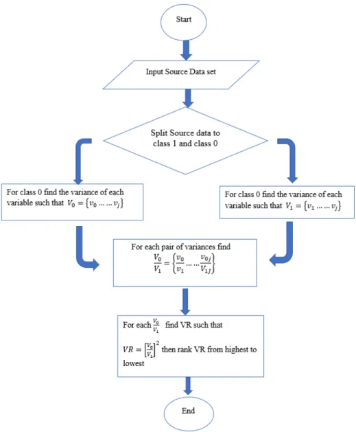
Collected data in Real-life that has not undergone any form of treatment are often referred to as raw or dirty data, it thus means that literally and logically. Its rawness stem from the fact that more often than not, it is not impossible to use such data without some forms of treatments, this is known as data processing. Data pre-processing is an extensive exercise that involves series of activities which depends on the type of problems identified in the raw data, some of the common prob-lems associated with raw data could be categorized into the following; Imbalanced classes, Structuralization, Data Cleaning, Data Transformations etc. Figure 1.1 is a representation of these problems

Figure 1.1: Problems of Real-Life data sets

1.1.1

Imbalanced class

This whole work is dedicated to the problems of imbalance classes in real-life data and it would be dealt with exhaustively in consequent sessions, meanwhile Figure1.1

with other problems, for example in a binary scenario (two-class -yes or no, 1 or 0) and even multi-classed (more than two classes) the data are usually not evenly divided. One group will always be dominant as such the sensitivities of most machine learning algorithms are always predicting more of the dominant group at the expense of the minority groups. The dominant groups with higher number are called majority class, while the smaller group are called minority class. The ratio of the majority class to the minority class is refers to as the imbalanced ratio(IR).

Imbalanced classed is not peculiar to only granular data, but many life scenarios have an imbalanced problem, below are some of the examples, but the list is endless.

• Oil spillage - in identifying oil spillage in the ocean, small area of image or water sample with the contamination compared to the large area of water without contamination produces an imbalanced image or data respectively.

• Tracking migrations of species like birds -Tracking migrations of species like birds; large areas of topography compared to a very small area dotted with migrating species produces an imbalanced image of topographical identifica-tions.

• In security image recognition - In the security image recognition; police tracking a single or few suspects by using a CCTV Camera in a crowd of people produce an imbalanced image recognition scenario.

• In health or intrusion data - The minority may be the few patients that have lung cancer compared to a large amount of data of patient without cancer or in intrusion detection data the few times that hackers have successfully breached the network compared to millions of successful login.

Traditional approaches to classifications in the context of imbalanced classed distributions in data sets has serious limitations, these will be introduced and dealt with very well in chapter 2 and later chapters, but Figure 1.1 have left us with compelling evidence of the the pervasiveness of the problem and how easily a data set which exhibit imbalance problems could be mistaken for other problems and vice versa. For example if a predictive modelling produces poor accuracy, this should raise some important questions like, is the poor accuracy due to missing values or other errors or due to uneven classes? What part of the poor performance are due to imbalanced classes and what parts are due to other problems? could the causes easily be identified ? eliminated or minimised?

scenario and manifest in what ever form is used to represent the scenario be it granular or non granular data. Most machine learning(ML)algorithm have proven inadequate [5] in dealing with the imbalanced. In the next sessions some of the errors associated with data sets but are not due to imbalance classes will be reviewed.

1.1.2

Data structuralization

This is the process of giving a structure to a collected data in a data set. The extent to which a dataset is organized is a measure of its level of structuralization, highly organized data set possibly stored in databases, flat files or others that enables manipulation of any sort, integration with other interfaces and software to aid and support exploitation with algorithms and other forms of data processing techniques with a view of extracting information and knowledge from the data are said to be structured [6]. On the other hand, Unstructured data are opposite of this, in that its a collection of data with no identifiable level of organizational formalism, hence Unstructured data cannot be manipulated, queried, integrate or worked on like Structured data.

One of the first activities of a Data Scientist is to improve the level of the structure of the collected data through formalizing the data items structural organizations based on the required and expected usage. Structuring the Unstructured data could be as simple as importing or exporting into a database table by tabulating it with identifiable rows and columns headings, another way may be exporting data into a text or Comma-separated values (CSV) files with identifiable columns and rows. Some could also involve using sophisticated processes and software that could enable any item in the data set to be identified and queried using unique metadata for extractions of a specific data item [7]. Whatever techniques used in structuring unstructured data, the result is that the data set will become more organized and any single data item could be identified and manipulated.

1.1.3

Dirty data

Is a term used in describing the different states of raw data that could impact on its quality, the dirty data must be clean by the process of detecting, correcting or removing inappropriate data item in the data set. To put it in perspective, what makes a data dirty? Dirty data are regarded as having the following common issues as listed below among many others.

• Incomplete data: If any position were a data item should be, have been left blank, nothing is written in the position.

• Duplicate data: mistakenly repeating row in a table more than once.

• Inaccurate data type: the data item input is not correct, for example, if the correct value for age is 36 year, but 360 is written.

• Incorrect data type: this is when wrong data types were used for example if for the age of a person is 36 years, an error was made by inputting the alphabet ”wy” in place of 36 due to typographic error.

1.1.4

Cleaning by data transformation

The first part of this transformation is known as unit integration where the unit of measurement of the variables must be equalized [8]. This part of Pre-processing data is usually bespoke and context-dependent because the data transformation is based on local rules and standard compliance [9]. For instance, in a data set that contains a variable of prices of item in Pound Sterling and USA Dollars must be transformed to the same Unit of Currency and scale because one USA Dollar is not equal to One Pound Sterling. Also if in a data set where Date is written in DD/MM/YY and is to be combined with another data set where the date DD/MM/YYYY, the proper transformations must be done before any data mining and machine learn-ing processes should be applied. The Unit integration processes are too numerous to mention but depend on local context and standard, mostly they are typically grouped into what is known as Extractions Transformation and Loading (ETL). Most data mining tools and software have ETL supporting facilities that do this, but the data scientist must know what data item is to be transformed and why.

1.1.5

Identifying outliers and noise

Outliers are values of a data item that are very much different from other values, but noise is wrong values though may appear as real values or may not, in any observation some values may be totally far away from others they are not wrong values these are Outliers, in most cases the observation differs so much from others hence become noticeable immediately [10]. For instance, if observations of adult age contain a value of 400 as age, this would arise suspicious because no living adult is as old as that, this is a noise because is a wrong value. For example, lets consider the average annual income of six middle class adult as $45000, $59000, $66000, $48000, $56000, $60000, $1500000 while most earned a five figure income the last person earned seven figure income, if this is correct such a data is an outlier because is remarkably different from the rest, but noise is just an incorrect data.

There are various ways to detect the presence of outliers in a data set, bar charts and histograms are one of the easiest ways of visually identifying the outliers in data sets. Another way of identifying suspected outlier is to use a statistical analysis known as

Interquartile Range (IQR). To find the (IQR) we have to define the following

terms Q1 which is the first quartile of all the data point from minimum, Q3 is the

third quartile of all the data point from the minimum. These are illustrated in Figure 1.2.

Figure 1.2: Interquartile Range

IQR =Q3−Q1 (1.1)

To deduce Outliers= Multiply 1.5 and IQR 1.5∗IQR

Upper Outliers are values greater than (1.5∗IQR) +Q3

Lower Outliers are values lower thanQ1−(1.5∗IQR)

Outliers could also be identified by using Box and Whiskers, Figure 1.3 is example of Box and Whiskers.

Outlier could be shown using Box and Whisker, in general the rule of thumb in identifying the outlier are data points that lie more than 1.5 IQR below the minor 1.5 IQR above themaxare most likely to be Outliers, but the red flag could also lie within Q1 and Q3 . Having been able to identify the outliers in your data set, the

implications and meaning of the outliers must be ascertained [11]. Is all Outliers a dirty data? the answers is ”NO”, you must infer if the outlier constitute a dirty data that must be corrected or done away with or it may be the ”gold” you are mining for.

In a variable of ages of adults, if a value of 500 as the age is identified, is very possible that it is an error and thus a dirty data for obvious reasons that no living person should have such age and it must be appropriately treated like replacing it or out-rightly removing it. But if the data set is for computer network intrusion

Figure 1.3: Box and Whiskers

detection, the outlier may represent the few times that hackers have breached the network, therefore such outlier may be the ”gold” you are mining for hence should be investigated further to ascertain what it stands for. It, therefore, comes down to the domain knowledge of Business Understanding to be able to explain the meaning and the implications of the discovered outliers or data items that are significantly different from others.

1.1.6

High dimensionality

To put it simply dimensionality refers to the number of attributes or features in a data set, if a data set is made of n rows; representing each data item and p columns representing features or attributes, the comparative values of sizes of n to p defines the order of dimensionality of the data set [12], while it has not been conclusively established the values of p that is high dimension due to context domain dependent, but is generally accepted that a data set is regarded as high dimension when p > n. In some areas like Bioinformatics, Astronomy, Image Recognition and Finance, data set with thousands of features are not uncommon [13], microarray which are used to measure expression level of gene, Deoxyribonucleic Acid(DNA)information are notoriously known for high dimensionality. The curse of dimensionality is the difficulty associated with extracting the required information from data set due to

the high dimensionality. Techniques for reducing the dimensionality of data set into manageable dimensions is an active areas of research, please see [14] [15] [16].

1.2

Motivation

This research is motivated by the inability of most predictive algorithm in dealing effectively with imbalanced classes in real-life data set. For the fact that imbalanced classed situations in context and concept are pervasive and recognizable in many aspects of our life, therefore providing solutions to this problem will greatly improve all aspects of predictive modeling. In both industries and academia, lots of predictive algorithms are used daily to solve problems or arrive at decisions but the performance of these algorithms varies in accuracy. These variations have been traceable to imbalanced class situational context. To be specific, this research is motivated by the following reasons.

• As depicted in Figure 1.1 imbalanced classed is a default problem that are always present in associations with other (one or more) raw data problems. Consequently, is a systematic error [17] [18] that is inherent in the dataset in combination to other errors that the datasets has. Therefore to say that if it is minimised or eliminated, the general result of all predictive modelling could improve will be an understatement.

• To bring it into situational perspective, this work quest to find the answers to questions like; “why is it that most algorithm could only predict less of the minority classes and in most cases far less than 30% of these minority”? [19], could these limitations in the predictions be attributed to the fault of the algorithms, wrong processes and techniques or because of an underlying characteristic of the data set, furthermore if imbalanced classes can never be eliminated, at what threshold of imbalanced ratio should the result of a classifier begins to loose its dependability, can we quantify these dependability in comparison to the imbalanced ratio?

• It is obvious that much of the general performance of most classifier are limited to their ability to deal with the imbalanced class issues, the data analysis life circle, that are often referred to as Cross Industry Standard Process for Data Mining (CRISP-DM) [20] is a bit silent in this regard for not factoring imbalanced classes to any of its stages, for this we wished to investigate and proffer solutions as to what stage imbalanced will be treated, more precisely we would delve into the applications of this(ML)algorithm and the relationship to

the properties of the data item, we would deduce a quantitative and qualitative generic influences of the algorithms and intrinsic data properties on the (IR)

and make recommendation on how to effectively treat imbalanced classes at the appropriate stage in the life circle.

• Imbalanced Ratio(IR) varies significantly, from moderate to severe so are the performance of the (ML) algorithms on the data during classification. But most research have visibly avoided to investigate the relationship of the de-gree of imbalanced to performance of classifiers. The research will establish the correlations of the variations of imbalanced to the properties of the data item and the performance of the (ML) on various levels of imbalance. This will enable overview of the expected performance to be estimated before a de-tailed analysis is carried out and also an informed decision on the type (ML), data preprocessing and many other activities that would make sensitivities of existing Machine learning(ML)to be able to target minority in an imbalanced dataset while eliminating the negative influenced of class imbalanced .

Special emphasis will be paid to both binary and multi-classed imbalance with a view of inventing a process that could be applied in both scenario ie binary and multi-classed data. Perhaps since imbalance classes problems cannot be completely eliminated but with the right processes the effects could be reduced to the barest minimum, for this we would produce a system where the threshold of dependable result will be known or estimated .

1.3

Aims

The aims of this research are to provide techniques to eliminate skewness of algo-rithms towards identifying more of the dominant majority group during the imbal-anced classes classification modelling. This will improve the accuracy and general predictive performance in both binary and multi-classed datasets. The ubiquitous nature of real-life datasets is such that a formalized approaches will be invented to find the threshold of imbalanced ratio at which a classifier results becomes less reliable. Finally, the correlation of the degree of overlapping and imbalance will be demonstrated, this will also help in minimising the skewness of algorithm towards capturing more of the dominant majority group(s) instead of the small minority classes that are usually the reasons for the predictive modelling.

1.4

Contributions

In course of achieving the research aims, new processes and procedures will be in-vented to provide alternatives to already existing techniques in dealing with imbal-ance data, the solutions we proffer here is a significant contribution, consequently, the work will itemize all major novelty and contribution as follows.

• This research produced a novel technique called Variance Ranking Attribute Selection (VR) to handle imbalanced classes in both binary and multiclass datasets. Though, it has been referred to as Variance Ranking in many in-stances through out this thesis. The superiority of the (VR) over the exist-ing techniques of dealexist-ing with class imbalanced have been demonstrated by producing better results, being able to deal with overlapping classes more ef-fectively and being algorithm independent. For the proof of concept (POC)

seven major dataset were used. These are further explained in chapter three session 3.1.1

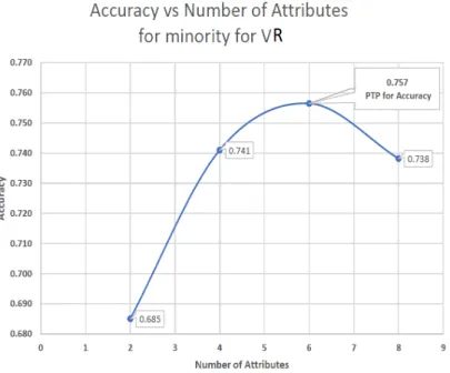
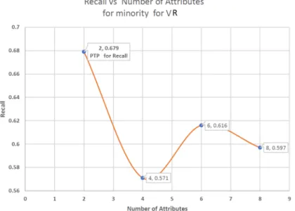
• A novel method of choosing significant attributes based on Peak Threshold Performance -(PTP), which is defined as the point at which the predictive model accuracy is at his highest, hence two types of(PTP) is identified these are (P T P)Accuracy and(P T P)minority. The(P T P)Accuracy is the point in the

predictive model were the highest accuracy occurred, while (P T P)minority is

the point at which the predictive model has the highest recall of the minority class group. This would also help to identify the threshold of attributes that are required to obtain dependable results based on the context of discourse and at the point where the significant attributes will be selected. These are further explained in chapter five from session 5.0.1 to section 5.0.20.

• An introduction to a new similarity measurement techniques called Ranked Order Similarity-(ROS), as a techniques to quantify the similarities among a sets of items that may contain the same elements but ranked in different order. To accomplished this, a novel distance measure called ”proximity distance” that assessed the distances of comparative items were defined. The (ROS) is a novel similarity measure that is applicable in situations where the existing similarity measure is inadequate for example were similarities is by ranked. These are further explained in chapter four session 4.4.

1.4.1

Terms Definitions

Effort have been made for all the invented (coined) words, phrases and nouns used in the thesis to have a specific meaning as will be explained wherever such words are used. When there are more than one words that refers to the same meaning and is unavoidable to used one of the word for example this three words refers to the same meaning; ”Variable”,”Attribute” and ”Feature”. The three words will be used interchangeably as it has always been used in most academic reports and journals and will comply to academic writing best practises.

One of the main concept is Variance Ranking Attributes selection(VR)and may be referred to as Variance, particularly in some table where there is no enough space. In any other places were any terms or words would appear differently the meaning will be obvious or it will be explained or defined appropriately. Reader’s attentions will be drawn to some common coined words that will be used through out this thesis, these are listed below.

• Peak Threshold Performance (PTP); this is the position that at which the highest accuracy and recall of the minority class groups were obtained. They are two types of (PTP), these are , (P T P)Accuracy and (P T P)minority.

• Element Percentage Weighting (EPW). This is the sum total percentage quan-tity of elements in two sets that are going to be compared; see section 4.4.

• Unit Element Percentage Weighting (EPW/n). This is the percentage weight-ing of a sweight-ingle element in a set; see section 4.4.

• proximity distance; this is the number of steps a Unit element in a set moves to align itself with a similar element in the another set, when both sets are being compared;see section 4.4.

1.5

Research Methodology

The goal of this research is to produce a process that could limit or eliminate the skewness of algorithm toward identifying more of the dominant majority group as against the smaller minority that are often sought when using imbalanced classed datasets. These goal has been fully articulated in the project specification vis-`a-vis the aims, and contributions therein. In so doing it will encompass every aspect of relevant discussions that will ensure a wholistic conclusion with adequate proof of validity, reliability of the assertions made in this document.

its objective are emphasised and not entwined in verbose research discourse [21], hence the general research methodology, the Proof of Concept (POC), results will be precise and straight to the point in order that the experiments could be replicated. The sequence of flow of the research will be in a particular order from inception to finish. Though these order boundaries are not strictly define, but to act as a guide to enable clarity, understanding, and coherency of thought. The sequence is as follows;

• Problem Definition and Specifications and introductions to the real life context of imbalanced data.

• Reviews of state of the art literature in dealing with imbalance data and met-rics of evaluating the Binary and Multi-classed data classifications.

• Data acquisition, preparations, and sampling methodology.

• The re-coding of multi-classed into n Binary, where n represent the number of classes in the multi-classed datasets.

• Experiment for Variance Ranking Attribute Selection Technique.

• Comparison of Variance Ranking Attribute Selection with two states of the art Attribute Selection using the Pearson Correlation (PC) and Information Gain (IG)

• Comparing the attributes ranked by (PC), (IG)and (VR) using the (ROS).

• Validation experiment of Variance Significant Ranking Attribute Selection us-ing some major(ML) algorithms.

• Comparison by estimating the degree of similarity Variance Ranking Attribute Selection with two sampling technique of dealing with class imbalance.

• Final discussion of results and conclusions.

Software, Hardware, and Algorithms

The list of all the major resources that were used in this research is as follows.

• Weka data mining software. That could be downloaded at [22].

• Python(v3) programming language. A very robust programming lan-guage for scientific computation and data analysis. As at the time of writing this thesis it has version 2 and version 3. The version used here is 3.

• Microsoft Office (Word, Excel, Paint, etc). A popular documentation for PC mac book.

• Datasetsall downloaded from [23]. This was downloaded from the university of California dataset archive.

• Hardware, PC and laptop. The only hardware used is PC,laptop with win10. There was no special capacity, any regular PC or laptop will do.

• Latex documentation. Thesis documentation carried out in Latex [24]. Though lots of latex editor online and those that could be installed on the desktops , but I had used specifically the online overleaf that have been cited earlier, I found it more convenient because being online made it accessible anywhere.

• Algorithms used. There are two major processes derived in this research, these are (VR) and (ROS). Each of these processes is as a result of other al-gorithms. The major algorithm that was used to derived the (VR) processes is one of the measure of central tendency called the ”Variance”, this is fur-ther explained in chapter three, session 3.1.1. The (ROS) is derived from the Levenshtein Similarity, this is futher explained in chapter four,session 4.3.1

A clear attempt will be made throughout this work to ensure that the aims, con-tributions, and processes being carried out are very clear to the reader sometimes through ”repetitions of the aims”, ”similar experimentation that emphasis the same results” and other techniques, this is to ensure that the conclusion will be proven beyond any reasonable doubt and to reinforce the sequence of understanding of the research work.

The work is for Doctor of Philosophy and every aspect of this work must be made to show deep thinking and originality and creation of knowledge. In presenting this documentation, It seek to make sure it complies to be ” Clear Precise and Accurate” according to [25].

1.5.1

List of Publication

• Ebenuwa, S.H., Sharif, M.S., Alazab, M. and Al-Nemrat, A., 2019. Variance ranking attributes selection techniques for binary classification problem in im-balance data. IEEE Access, 7, pp.24649-24666.

• Ebenuwa, S.H., Sharif, M.S., Al-Nemrat, A., Al-Bayatti, A.H., Alalwan, N., Alzahrani, A.I. and Alfarraj, O., 2019. Variance Ranking for Multi-Classed

Imbalanced Datasets: A Case Study of One-Versus-All. Symmetry, 11(12), p.1504.

1.5.2

Summary of Thesis Report Layout

Chapter One(Introduction). In the introduction, we made the case for the

research topic by introducing the background of the study as being the general problems encountered when working with real-life datasets. The positing of imbal-anced classes as being very prevalent in additions to other real-life dataset issues was made here. A detailed explanations of other data sets issues as an addition to imbalanced class was presented. Furthermore, an explanation of similar imbalanced scenario, processes of dealing with raw data. Clear problems definition by explaining the research motivation, aims and contribution to knowledge was firmly rooted in this chapter.

Chapter Two(literature Review). The chapter is an extensive presentation

of previous work that has been done in dealing with imbalanced class distribution in data sets, we engage the argument of using data-centric research like data mining and machine learning to provide a solution in real-life scenario, hence the extent and attempt that has been made to provide solutions were explored here in a broader per-spective. The metrics of evaluations for classifiers were introduced for both binary and multi-classed data sets, we provided detailed explanation for 2 by 2 confusion matrix for binary classification and One-Versus-All for multi-classed scenario

Chapter Three(Variance Ranking Attribute Selection (VR)

Tech-nique)In this chapter we presented the Variance Ranking Attribute Selection

tech-nique for handling the imbalanced classed distribution, a detailed explanations of the datasets and data preparations, the theoretical basis of formula derivative used throughout the report and the experiments result were also included in this chapter.

Chapter Four(Comparison of Variance Ranking Attribute Selection

(VR) Technique with the Bench Mark) In this chapter a comparison of

Vari-ance Ranking Attribute Selection(VR) and other bench mark in attribute selection is provided , also a new similarity measurement techniques ”The Ranked Order Similarity measurement-ROS” was used to compare and quantify the similarities between the Variance Ranking Attribute Selection (VR)and two main bench marks which are Pearson Correlation and Information Gain. The novelty of The Ranked

Order Similarity measurement-ROS was invented here.

Chapter Five(Validation) In this chapter predictive modelling experiments

were carrieed out using three machine learning algorithm and seven data set (four binary and three multi classed). The accuracy , precision , recall etc were noted. The capturing of the minority class group in the imbalanced situation were proven, hence attesting to the efficacy of the (VR) techniques. More importantly, the com-parison of Variance Ranking with(SMOTE)and ADASYN techniques. The chapter provided and consolidated the reasons for the failure of using the algorithm based methods which have been the the conventional means and made a case why the

(VR),(SMOTE)and (ADASYN)techniques that rely mostly on the numbers of the

class groups is the right approaches to use.

Chapter Six (Summary Discussion and Conclusions) This chapter

high-lighted the major achievements of the research with a blow by blow summary of how the aims, and contributions were achieved, we also highlighted the shot comings of the existing techniques of handling the imbalanced data set problems. We provided a distinctive yet succinct presentations of all aspects of research that that made it possible to any reader to be familiar with the central knowledge that have been claimed achieved, we made ac case for the relevance of (VR)and the future work.

Literature Review

2.1

Overview of imbalance data

Class imbalance is a major problem in using real-life data for predictive modelling. A data set is said to be imbalanced when there is unequal number of groups, mean-ing that one group is more than the others, the larger groups are the majority classes while the smaller groups are called the minority classes, the ratio of the majority class to the minority class is often referred to as the imbalance ratio (IR) in binary classed imbalanced data. In the multi-classed imbalanced, the (IR) will be defined according to the techniques that will be used to express the imbalanced, the Figure

2.1 is a representation of different types of imbalance, for the binary classed, the

(IR) is 9:1 or 90%, this is straight forward. But for the multi-classed, the (IR) is 50:30:10:5:3:2, to expressed the(IR)as a percentage will depend on the technique of decomposition of the multi-classed using either ”one-versus-one” or ”one-versus-all” please see sections 2.3.2.

The problems caused by imbalance classes could affect all known predictive cate-gories; like supervised, unsupervised, and hybrid. In supervised learning, classifi-cation could be multi-classed or binary classed, the multi-class is when the target groups are more than two while binary is when the target groups are only two (Yes or No, Positive or Negative), [26] [27].

The effect of class imbalance in binary context is that, the accuracy of the predic-tion could be as high as 90% yet no minority class group has been captured by the prediction [28]. For example, if a data set has a total of 1000 instances, assuming that 900 are negative while 100 are positive case, if a binary classification predicted all the 1000 cases as negative will still appear to be 90% accurate, whereas none of the 100 minority class group have been captured.

Figure 2.1: Imbalanced and Balance data

The same wrong predictions in binary class is also very noticeable in a multi-classed data as shown in Figure2.1, consider a data set with classes as follows 50%, 30%, 10%, 5%, 3%, 2% being able to predict the small percentage groups (minority classes) by using the conventional machine learning algorithm and processes is next to impossible because by design and applications these algorithms assumed equal classes, and during implementations the process is usually optimized for accuracy thereby enhancing the capturing of the same majority classes. The irony is that, in most prediction; binary or multi-classed using real-life data, the minority groups are usually the interest or what we are looking to predict. Consider the case of binary classification in intrusion detection dataset. The minority is the few times the net-work may have been breached, in cancer research dataset, the minority group may be the few patients that have cancer, while in clinical trial of drug interactions, the few adverse interactions are usually the interest groups. In a multi-classed dataset were the prediction of various numbers in group membership is required like the ages of Abalones based on the numbers of rings [29], predicting a protein localization site in the Deoxyribonucleic acid(DNA)[30]. The smaller groups are impossible to cap-ture using the conventional machine learning algorithm and processes.

It is quite obvious that if a technique could be found to eliminate the problems of class imbalance, the performance of most predictive algorithm will improve dras-tically. At this juncture, let us provide a precise definition of the term predictive modelling. What is predictive modelling? ”This a term used to describe processes and techniques that use Statistics and machine learning to predict future events, outcomes or items, while using earlier events, data or observations as inputs during the process.”

2.2

Techniques for handling imbalance class

dis-tribution

Imbalance classes have been a problem in predictive modelling when using the con-ventional machine learning algorithm consequently have been a subject of interest in both the academia and industries, different approaches have been proposed to han-dle this problem with different level of successes. Each of these approaches could be categorized as Machine Learning Algorithm methods, Cost-Sensitive methods, Embedded Approaches, and Sampling-based Methods. In the preceding sections, details of these approaches will be dealt with.

Before delving into these approaches, it is important to have an overview of the gen-eral commonality to all of them in context. First and foremost, all the approaches involves the machine learning algorithms at some points in the processes, but the stress on names of the categories is to emphasis the deliberate efforts that have been made to alter, combine or improve the machine learning algorithms for the sole purpose of improving the accuracy of the results or general performance using the standard measurement metrics.

The default predictive modelling techniques is to use machine learning algorithms, data scientist uses algorithms and modifications of parameters to obtain some accu-rate results, it was not intended to actually solve the problems of imbalance classes because the numbers of classes that made the dataset imbalanced were not con-sidered when using this approaches, but since it sometimes achieved good results particularly when the data are imbalanced it became the norms. The parame-ter changes like changing the kernel functions in (SVM) and other unstandardized processes became the conventional way of modelling with imbalance data (afterall almost all real-life data set are imbalanced). Other approaches, like the Embedded Approaches and Cost-Sensitive methods, uses the same modification of the algorithm methods. These parameter changes and different ”tweaking” of the algorithms are one of the origins of the ”trial and error” that has become a well-known process in data mining and machine learning methodology [31][32][33].

The first effort that was made to target imbalance classes in real-life data was car-ried out by using sampling methods (Over Sampling and Under-Sampling). Though different modifications of these Sampling methods have evolved over time. Section

2.2.6and chapter 6 are fully dedicated to these techniques, and a detailed discussion

2.2.1

Overview of machine learning algorithm

In general, the algorithms used in data science are categorized into supervised and unsupervised learning, as depicted in Figure2.2. While supervised learning are used when the target output Y is already known, the algorithm have to be trained to learn the functionF that is used to map the input X to the output, represented as

Y =F(X), hence it shows that any series of input X ={x1, x2, x3...xn} could be

used to predict a series of outputY ={y1, y2, y3...yn}using a mapping functionF

[34]. Therefore, all supervised learning has a set of training input that is “learned” by the algorithm to produce a generic mapping function that will be used to map all the input to the various output target. The supervised learning is further classified into two according to the nature of the output target being sort; if the output target is discrete like yes or no, male or female, have the disease or don’t have the disease, high or middle or low, there are called classification. The other type of supervised learning is called regression in nature if the output could be a real number like the following continuous values 56.34, 123.03, 0.34.

Figure 2.2: Machine learning algorithm

[35]. It involves the input data being exposed to the machine learning algorithm enabling it to find the previously unknown pattern in the input data. These hidden patterns are usually invisible before being exposed to the algorithm, hence the term mining. Most unsupervised learning algorithms are categorized as being clustering or associations pattern-based. Therefore when the input data interacts with the algorithm, clusters of data that share similar characteristics are noticed. In the same way, if a data item is related to another data item by any associations, a rule-based algorithm would expose the pattern. Semi-supervised learning is a hybrid of supervised and unsupervised learning [34].

2.2.2

Variance Techniques For Handling imbalanced classed

data

This is one of the approaches for dealing with imbalanced classed datasets, the variance is always used in combination with other intrinsic properties of the data [36][37]. This research is based on this approach by using the variance to derived the feature that are most significant to eliminate or reduce skewness of the (ML)

toward identifying more of the majority class as against the minority class.

The work of [38] provided a pointer as to how variance and feature selection could lead to improved performance in classification. The work demonstrated a techniques known as a Sensitivity Analysis (SA) which is based on Fourier amplitude test. The Fourier test is depended on the variance test of the amplitude function of wave, but the authors were able to applied this to Feedforward Neural Network (FNN) thereby showing that the classes of datasets relatively depended on their variances and this correlations was used to select the significant features. The results obtained showed an improvements in the classifications, but the issues of skewness still remains, par-ticularly in the highly overlapped datasets.

In order to assess the levels of imbalanced quantitatively [39] developend a method called ”Bayes Imbalance Impact Index”, this techniques uses two metric called ”Indi-vidual Bayes Imbalance Impact Index-(IBI3)” and ”Bayes Imbalance Impact Index-(BI3)”. The IBI3 and BI3 are used to a measure the effects of imbalance on vari-ables as the degree of imbalance increases. The authors also provided a prove to show that if the datasets are normally distributed, the probability density functions and the likelihood of finding a data item in the sample space could be deduced from the mean and variance. Therefore a strong correlation between (IBI3) and variances of the distribution was established.