Durham Research Online
Deposited in DRO:04 June 2014
Version of attached le:
Accepted Version
Peer-review status of attached le:
Peer-reviewed
Citation for published item:
Coolen-Maturi, T. and Elkha, F.F. and Coolen, F.P.A. (2014) 'Three-group ROC analysis : a nonparametric predictive approach.', Computational statistics data analysis., 78 . pp. 69-81.
Further information on publisher's website:
http://dx.doi.org/10.1016/j.csda.2014.04.005 Publisher's copyright statement:
NOTICE: this is the author's version of a work that was accepted for publication in Computational Statistics Data Analysis. Changes resulting from the publishing process, such as peer review, editing, corrections, structural
formatting, and other quality control mechanisms may not be reected in this document. Changes may have been made to this work since it was submitted for publication. A denitive version was subsequently published in Computational Statistics Data Analysis, 78, 2014, 10.1016/j.csda.2014.04.005.
Additional information:
Use policy
The full-text may be used and/or reproduced, and given to third parties in any format or medium, without prior permission or charge, for personal research or study, educational, or not-for-prot purposes provided that:
• a full bibliographic reference is made to the original source • alinkis made to the metadata record in DRO
• the full-text is not changed in any way
The full-text must not be sold in any format or medium without the formal permission of the copyright holders. Please consult thefull DRO policyfor further details.
Three-group ROC analysis:
A nonparametric predictive approach
Tahani Coolen-Maturia, Faiza F. Elkhafifib, Frank P.A. Coolenc,∗
aDurham University Business School, Durham University, Durham, DH1 3LB, UK bDepartment of Statistics, Benghazi University, Benghazi, LIBYA
cDepartment of Mathematical Sciences, Durham University, Durham, DH1 3LE, UK
Abstract
Measuring the accuracy of diagnostic tests is crucial in many application areas, in particular medicine and health care. The receiver operating char-acteristic (ROC) surface is a useful tool to assess the ability of a diagnostic test to discriminate among three ordered classes or groups. In this paper, nonparametric predictive inference (NPI) for three-group ROC analysis is presented. NPI is a frequentist statistical method that is explicitly aimed at using few modelling assumptions in addition to data, enabled through the use of lower and upper probabilities to quantify uncertainty. It focuses ex-clusively on a future observation, which may be particularly relevant if one considers decisions about a diagnostic test to be applied to a future patient. This paper presents the NPI approach to three-group ROC analysis, includ-ing results on the volumes under the ROC surfaces and choice of decision thresholds for the diagnosis.
Keywords: Diagnostic accuracy, Lower and upper probability, Nonparametric predictive inference, Receiver operating characteristic (ROC) surface, Youden’s index.
∗Corresponding author
Email addresses: [email protected](Tahani Coolen-Maturi),
[email protected](Faiza F. Elkhafifi),[email protected] (Frank P.A. Coolen)
1. Introduction
Measuring the accuracy of diagnostic tests is crucial in many applica-tion areas, in particular medicine and health care (Wians et al., 2001; Pepe, 2003; Xiong et al., 2007; Lopez-de Ullibarri et al., 2008; Tian et al., 2011; Rodriguez-Alvarez et al., 2011a,b; Chen et al., 2012), the same statistical methods are used in other fields such as credit scoring (Xanthopoulos and Nakas, 2007). Good methods for determining diagnostic accuracy provide useful guidance on selection of patient treatment according to the severity of their health status. The receiver operating characteristic (ROC) surface is a useful tool to assess the ability of a diagnostic test to discriminate among three ordered classes or groups. The construction of the ROC surface based on the probabilities of correct classification for three classes has been intro-duced by Mossman (1999), Nakas and Yiannoutsos (2004) and Nakas and Alonzo (2007). They also considered the volume under the ROC surface (VUS) and its relation to the probability of correctly ordered observations from the three groups. The three-group ROC surface generalizes the popular two-group ROC curve, which in recent years has attracted much theoretical attention and has been widely applied for analysis of accuracy of diagnostic tests (Zhou et al., 2011; Zou et al., 2011).
Statistical inference for accuracy of diagnostic tests using ROC curves or surfaces has mostly focused on estimating the relevant probabilities of correct classification for the different groups, with these probabilities being considered as properties of assumed underlying populations. While this is a well-established approach, with methods presented for fully parametric models as well as semiparametric and nonparametric methods (Heckerling, 2001; Li and Zhou, 2009), the practical importance of diagnostic tests is in their use for future patients. As such, it is of interest to study a predictive statistical approach to such inferences on accuracy of diagnostic tests. The importance of prediction is well understood, e.g. Airola et al. (2011) and van Calster et al. (2012) explicitly mention ‘predictive models’ and ‘prediction models’, but thus far the statistical approaches used in this field have mostly been based on estimation, with their predictive performance investigated via numerical studies.
Nonparametric predictive inference (NPI) is a frequentist method using few modelling assumptions, and hence is strongly data-driven, which is en-abled by the use of lower and upper probabilities to quantify uncertainty (Augustin and Coolen, 2004; Coolen, 2006, 2011). Lower and upper
proba-bilities generalize the classical theory of (precise) probability (Coolen et al., 2011), with the difference between the upper and lower probabilities for an event typically reflecting the amount of information available. In NPI, the lower and upper probabilities always provide bounds for empirical probabil-ities, hence the NPI-based statistical conclusions are never contradictory to those based on empirical probabilities (Coolen, 2006). Due to the impor-tance of prediction of the accuracy of diagnostic tests for a future patient, NPI provides an attractive alternative approach to the established methods in this field. NPI has recently been introduced for assessing the accuracy of a classifier’s ability to discriminate between two groups for binary data (Coolen-Maturi et al., 2012a), ordinal data (Elkhafifi and Coolen, 2012) and real-valued data (Coolen-Maturi et al., 2012b).
This paper introduces NPI for three-group ROC analysis for real-valued data. Section 2 presents an introduction to three-group ROC analysis, fol-lowed in Section 3 by a brief introduction to NPI. NPI for three-group ROC analysis is presented in Section 4 and illustrated by an example in Section 5. The paper ends with concluding remarks in Section 6 and two appendices containing proofs.
2. Three-group ROC analysis
In this section we introduce the concepts and notation of three-group ROC analysis (Mossman, 1999; Nakas and Yiannoutsos, 2004; Nakas and Alonzo, 2007). Consider three groups, denoted byGx,Gy andGz.
Through-out this paper, we assume that these groups are fully independent, in the sense that any information about one of the groups does not hold any infor-mation about another group. Let real-valued observed test results be denoted byx1, x2, ..., xnx for groupGx,y1, y2, ..., yny for groupGy andz1, z2, ..., znz for
groupGz. Suppose that a diagnostic test is used to discriminate the subjects
from these groups. We assume that the three groups are ordered in the sense that observations from group Gx tend to be lower than those from group
Gy, which in turn tend to be lower than those from group Gz. There will
typically be overlap of observations from different groups, but the practical diagnostic setting is assumed to be such that observations from the three groups tend to be ordered in this way. The cumulative distribution function (CDF) for the test outcomes of group G· is denoted byF·.
Two decision thresholds c1 < c2 are required to classify a subject into
for subject j: Subject j is classified into group Gx if Tj ≤ c1, group Gy if
c1 < Tj ≤ c2 and group Gz if Tj > c2. The test data are assumed to consist
of measurements for individuals known to belong to specific groups, while the goal of the inferences is to develop a diagnostic classification method for individuals for who the group is unknown. We assume throughout the paper that the test data do not contain errors.
Denoting the classification measurement random quantity for a subject from group Gx, Gy, Gz by X, Y, Z, respectively, the corresponding
proba-bilities of correct classification with thresholds (c1, c2) are p1 =P(X ≤c1) =
Fx(c1), p2 = P(c1 < Y ≤ c2) = Fy(c2)−Fy(c1) and p3 = P(Z > c2) =
1−Fz(c2). The ROC surface, denoted by ROCs, is constructed by plotting
the triples (p1, p2, p3) for all real-valuedc1 < c2. A convenient way to define
this ROC surface is as follows, for p1, p3 ∈ [0,1] (Inacio et al., 2011; Nakas
and Yiannoutsos, 2004; Tian et al., 2011), ROCs(p1, p3) = Fy(Fz−1(1−p3))−Fy(Fx−1(p1)) if Fx−1(p1)≤Fz−1(1−p3) 0 otherwise (1) where F−1
· (p) is the inverse function of the CDF F·.
The empirical estimator of the ROC surface can be obtained by replacing the CDFs in (1) with their empirical counterparts (Beck, 2005; Inacio et al., 2011), so for p1, p3 ∈[0,1], [ ROCs(p1, p3) = ˆ Fy( ˆFz−1(1−p3))−Fˆy( ˆFx−1(p1)) if ˆFx−1(p1)≤Fˆz−1(1−p3) 0 otherwise (2) where ˆFx−1(p) =xi if p∈(in−x1,nix],i= 1, . . . , nx, and ˆFx−1(p) =−∞if p= 0,
with ˆFz−1(p) defined similarly.
The volume under the ROC surface (VUS) is a global measure of the test’s ability to discriminate between the three groups. The VUS is equal to the probability that three independent randomly selected measurements, one from each group, are correctly ordered, so that the observation from Gx is
less than the observation from Gy and the latter is less than the observation
from Gz (Mossman, 1999; Nakas and Yiannoutsos, 2010). An unbiased
non-parametric estimator of the VUS is given by (Nakas and Yiannoutsos, 2004, 2010) [ V U S = 1 nxnynz nx X i=1 ny X j=1 nz X l=1 I(xi < yj < zl) (3)
withI(A) equal to 1 ifAis true and 0 else. Equation (3) gives the proportion of all possible triple combinations from the data that are correctly ordered, it is the empirical probability for this event based on the information from the data. It is (about) equal to 1/6 if the diagnostic test outcomes for the three groups completely overlap, in which case the data suggest that the test is not useful for the diagnosis. Perfect separation of the test results for the three groups, that is xi < yj < zl for alli,j and l, leads toV U S[ = 1. In practice,
ties between measurements may occur, in this case a modified version of (3) should be used (Nakas and Yiannoutsos, 2004, 2010). In this paper, for ease of presentation we assume that no ties occur in the data.
Several approaches for choosing the thresholds c1 and c2 have been
pro-posed in the literature (Greiner et al., 2000; Schafer, 1989; Yousef et al., 2009; Lai et al., 2012). We consider maximisation of Youden’s index (Youden, 1950), which for three-group diagnostic tests was introduced by Nakas et al. (2010),
J(c1, c2) = P(X ≤c1) +P(c1 < Y ≤c2)−P(Z ≤c2) + 1
=Fx(c1) +Fy(c2)−Fy(c1)−Fz(c2) + 1 (4)
J(c1, c2) is equal to 1 ifFx,Fy and Fz are identical, perfect separation of the
groups, P(X < Y < Z) = 1, leads toJ(c1, c2) = 3.
3. Nonparametric predictive inference
Nonparametric predictive inference (NPI) (Augustin and Coolen, 2004; Coolen, 2006, 2011) is based on the assumption A(n) proposed by Hill (1968).
LetX1, . . . , Xn, Xn+1 be real-valued absolutely continuous and exchangeable
random quantities. Let the ordered observed values of X1, X2, . . . , Xn be
denoted by x1 < x2 < . . . < xn and let x0 = −∞ and xn+1 = ∞ for
ease of notation. We assume that no ties occur; ties can be dealt with in NPI by assuming that tied observations differ by small amounts which tend to zero (Coolen, 2006). For Xn+1, representing a future observation, A(n)
partially specifies a probability distribution by P(Xn+1 ∈ (xi−1, xi)) = n+11
for i = 1, . . . , n+ 1. A(n) does not assume anything else, it is a post-data
assumption related to exchangeability (De Finetti, 1974). It is convenient to introduce the set of precise probability distributions which correspond to the partial specification byA(n), so which have probability n+11 in each of the
n+ 1 intervals (xi−1, xi). This set is called a ‘structure’ by Weichselberger
Inferences based on A(n) are predictive and nonparametric, and can be
considered suitable if there is hardly any knowledge about the random quan-tity of interest, other than the n observations, or if one does not want to use any such further information in order to derive at inferences that are strongly based on the data. The assumption A(n) is not sufficient to derive
precise probabilities for many events of interest, but it provides bounds for probabilities via the ‘fundamental theorem of probability’ (De Finetti, 1974), which are lower and upper probabilities in interval probability theory (Au-gustin and Coolen, 2004; Walley, 1991; Weichselberger, 2000, 2001; Coolen et al., 2011).
In NPI, uncertainty about the future observation Xn+1 is quantified by
lower and upper probabilities for events of interest. Lower and upper prob-abilities generalize classical (‘precise’) probprob-abilities. A lower (upper) proba-bility for event A, denoted byP(A) (P(A)), can be interpreted as supremum buying (infimum selling) price for a gamble on the event A (Walley, 1991), or just as the maximum lower (minimum upper) bound for the probability of A that follows from the assumptions made. This latter interpretation is used in NPI (Coolen, 2006, 2011). We wish to explore application of A(n)
for inference without making further assumptions. So, NPI lower and upper probabilities are the sharpest bounds on a probability for an event of interest when only A(n) is assumed. Using the A(n)-based structure, the NPI lower
and upper probabilities for event A are P(A) = inf
P∈Px
P(A) and P(A) = sup
P∈Px
P(A)
P(A) (P(A)) can be considered to reflect the evidence in favour of (against) event A (Coolen et al., 2011). Augustin and Coolen (2004) proved that NPI has strong consistency properties in the theory of interval probability (Walley, 1991; Weichselberger, 2000, 2001; Coolen et al., 2011), it is also ex-actly calibrated from frequentist statistics perspective (Lawless and Fredette, 2005), which allows interpretation of the NPI lower and upper probabilities as bounds on the long-term ratio with which the event Aoccurs upon repeated application of this statistical procedure.
4. NPI for three-group ROC analysis
In this section, NPI for three-group ROC analysis is presented. Notation is introduced in Section 4.1, which includes the introduction of the NPI-based
structures for the next observation from each of the three groups. In Section 4.2 the lower and upper envelopes of the set of all ROC surfaces corresponding to probability distributions in these NPI-based structures are derived by pointwise optimisation. These envelopes represent this set well, but they are too wide in the sense that the volumes under their surfaces are not generally the infimum and supremum of the volumes under the ROC surfaces in this set. To define NPI lower and upper ROC surfaces such that the volumes under them are equal to this infimum and supremum, respectively, we consider the relation between the volume under an ROC surface and the probability of correctly ordered observations from the three groups. The NPI lower and upper probabilities for this event are presented in Section 4.3, with the corresponding NPI lower and upper ROC surfaces presented in Section 4.4. In Section 4.5 the choice of decision threshold for the diagnosis is considered. As computation of the NPI lower and upper ROC surfaces is not straightforward, it may be attractive to quickly derive bounds for them. The envelopes presented in Section 4.2 provide a lower bound for the NPI lower ROC surface and an upper bound for the NPI upper ROC surface. In Section 4.6 we present a quick way to derive an upper bound for the NPI lower ROC surface and a lower bound for the NPI upper ROC surface.
4.1. Notation
To develop the NPI approach for three-group ROC analysis, let Xnx+1,
Yny+1 and Znz+1 be the next observations from groups Gx, Gy and Gz,
re-spectively. We apply A(n) for each group. Let the nx ordered observations
from group Gx be denoted by x1 < x2 < . . . < xnx and let x0 = −∞ and
xnx+1 = ∞ for ease of notation. For Xnx+1, representing a future
obser-vation from group Gx, A(nx) partially specifies a probability distribution by
P(Xnx+1 ∈(xi−1, xi)) =
1
nx+1 fori= 1, . . . , nx+ 1. For groupsGy andGz the
same concepts are introduced, with the obvious changes to notation. The sets of all probability distributions that correspond to these partial specifications forXnx+1,Yny+1 andZnz+1, are the NPI-based structures and are denoted by Px,Py and Pz, respectively. Forx∈[xi−1, xi) the NPI lower CDF for Xnx+1
isFx(x) = ni−1
x+1,i= 1, . . . , nx+ 1, and for x∈(xi−1, xi] the NPI upper CDF
for Xnx+1 is Fx(x) =
i
nx+1, i = 1, . . . , nx+ 1. Note that there is no
impre-cision at the xi, as Fx(xi) = Fx(xi) = nxi+1 for i = 0,1, . . . , nx + 1. These
lower and upper CDFs are derived as the pointwise infima and suprema over all corresponding CDFs in the structurePx. The NPI lower and upper CDFs
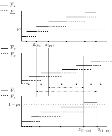
Figure 1: Construction of lower and upper envelopes of the set of NPI-based ROC surfaces
4.2. Lower and upper envelopes of the set of NPI-based ROC surfaces
For each combination of probability distributions for Xnx+1, Yny+1 and
Znz+1 in Px, Py and Pz, respectively, the corresponding ROC surface as
presented in Equation (1) can be created, leading to a set of NPI-based ROC surfaces, which we denote bySroc. The lower and upper envelopes of this set,
which consist of the pointwise infima and suprema, are presented in Theorem 4.1. First their construction is explained using Figure 1.
To derive the lower and upper envelopes of the setSroc, we need to derive
the infima and suprema of the values ROCs(p1, p3) for ROC surfaces in the
setSroc. Consider a value forp1 ∈(0,1) that is not equal to a valuei/(nx+1)
for anyi∈ {1, . . . , nx}. There is a uniquei∈ {1, . . . , nx+1}such thatxi−1 <
F−1
x (p1)< xi for every CDFFx corresponding to all probability distributions
x(p1), respectively, soFx(x(p1))< p1 < Fx(x(p1)) for the CDFs corresponding
to all probability distributions in Px. For p1 = nxi+1, for any i∈ {1, . . . , nx},
we would havexi−1 < Fx−1(p1)< xi+1, for ease of presentation we neglect this
as it only describes the envelopes at a finite number of observations. For the volumes under these lower and upper envelopes of all the ROC surfaces in
Sroc, which we consider later, it is also irrelevant what happens at this finite
number of points. Similarly, consider a value p3 ∈ (0,1) which is not equal
to a valuel/(nz+ 1) for anyl ∈ {1, . . . , nz}. We now consider all the inverse
CDFs F−1
z , corresponding to all probability distributions in Pz, and we are
interested in their value at 1−p3. There are two consecutive observations,
which we denote by z(1−p3) and z(1−p3), with z(1−p3) < F
−1
z (1−p3)< z(1−p3)
and therefore Fz(z(1−p
3)) < 1− p3 < Fz(z(1−p3)). We can again neglect
values of p3 such that 1 −p3 = nzl+1 for any l ∈ {1, . . . , nz}, for which
zl−1 < Fz−1(1−p3)< zl+1.
For any (p1, p3) as described above, the infimum of the valuesROCs(p1, p3),
as given by Equation (1), for all ROC surfaces in the set Sroc, can be
de-rived as follows (see Figure 1). We must find the infimum for the NPI-based probability for the event Yny+1 ∈ (x(p1), z(1−p3)), this interval corresponding
to the inverse CDFs is as small as possible. This is achieved by counting the number of intervals (yj−1, yj) that are totally included in (x(p1), z(1−p3)). We
denote the resulting lower envelope at the point (p1, p3) by ROCLs(p1, p3), it
is presented in Theorem 4.1. To derive the upper envelope, the interval cor-responding to the inverse CDFs is taken as large as possible, (x(p1), z(1−p3)),
and the NPI upper probability for the event that Yny+1 will be in this
in-terval is calculated by counting the number of inin-tervals (yj−1, yj) that have
non-empty intersection with (x(p1), z(1−p3)). We denote the resulting upper
envelope at the point (p1, p3) by ROC U
s(p1, p3), it is also presented in
The-orem 4.1. No formal proof of this theThe-orem is included, the steps follow the explanation just given, the theorem applies formally to the values of (p1, p3)
as described above.
Theorem 4.1. The lower envelope of all NPI-based ROC surfaces in Sroc is
ROCLs(p1, p3) = Fy(z(1−p 3))−Fy(x(p1)) if Fy(z(1−p3))≥Fy(x(p1)) 0 otherwise (5)
The upper envelope of all NPI-based ROC surfaces in Sroc is
ROCUs(p1, p3) =
Fy(z(1−p3))−Fy(x(p1)) if x(p1) ≤z(1−p3)
0 otherwise (6)
It is interesting to consider the volumes under these lower and upper envelopes, which we denote by V U SL and V U SU, respectively. These are given in Theorem 4.2, see Appendix A for the proofs.
Theorem 4.2. The volumes under the lower and upper envelopes of all NPI-based ROC surfaces in Sroc are
V U SL=A nx+1 X i=1 ny+1 X j=1 nz+1 X l=1 I(xi < yj−1∧yj < zl−1) (7) V U SU =A nx+1 X i=1 ny+1 X j=1 nz+1 X l=1 I(xi−1 < yj∧xi−1 < zl∧yj−1 < zl) (8) where A= (n 1 x+1)(ny+1)(nz+1).
These lower and upper envelopes of all NPI-based ROC surfaces in Sroc
are themselves not elements of Sroc. The minimisation performed to find the
lower envelope at (p1, p3) involves putting the minimum possible NPI-based
probability mass forYny+1 in the interval (x(p1), z(1−p3)). This pointwise
opti-misation gives, for all such points (p1, p3), solutions that cannot be obtained
simultaneously, particularly because it always minimizes probability mass for Yny+1 and hence, when all the solutions are taken together, not a total
probability of 1 is used for Yny+1. With regard to Xnx+1 and Znz+1 this
problem does not occur, as all optimisations with regard to the probability distributions for these random quantities have solutions that can be obtained simultaneously by either putting all probability masses to the left-end points or all to the right-end points of their intervals. These envelopes adequately describe the whole set of all NPI-based ROC surfaces in Sroc, but are in
generally equal to the infimum and supremum of the volumes under all the NPI-based ROC surfaces in Sroc.
We wish to identify ROC surfaces corresponding to Sroc such that their
VUS values are equal to the infimum and supremum of the VUS values for all the ROC surfaces in Sroc. We present this in Section 4.4, by focusing
on the volumes under the ROC surfaces and their relations to NPI lower and upper probabilities for correctly ordered observations, so for the event Xnx+1 < Yny+1 < Znz+1. However, as the NPI lower and upper probabilities
for such correctly ordered observations have not yet been presented in the literature, they are first derived in Section 4.3.
4.3. NPI lower and upper probabilities for the event Xnx+1 < Yny+1 < Znz+1
We present the NPI lower and upper probabilities for the eventXnx+1 <
Yny+1 < Znz+1, with notation as introduced in Section 4.1. These NPI lower
and upper probabilities for a specific ordering of three such future observa-tions have not yet been presented in the literature and can be applied to a variety of problems beyond their use in Section 4.4. They are not expressable in closed form, but are derived as follows.
Theorem 4.3. The NPI lower and upper probabilities for the eventXnx+1 <
Yny+1 < Znz+1 are P(Xnx+1 < Yny+1< Znz+1) = A nx+1 X i=1 ny+1 X j=1 nz+1 X l=1 I(xi < tjmin < zl−1) (9) P(Xnx+1 < Yny+1< Znz+1) = A nx+1 X i=1 ny+1 X j=1 nz+1 X l=1 I(xi−1 < tjmax< zl) (10) where A= (n 1 x+1)(ny+1)(nz+1) and t j
min (tjmax ) is any value belonging to a
sub-interval of (yj−1, yj), forj = 1, . . . , ny+ 1, where the sub-intervals are created
by the observations from groups Gx and Gz within this interval (yj−1, yj),
such that the probability for the event Xnx+1 < Yny+1 < Znz+1 is minimal
(maximal).
These NPI lower and upper probabilities are the infimum and supremum, respectively, over all precise probabilities for this event, corresponding to
precise probability distributions for Xnx+1 in Px, Yny+1 in Py and Znz+1 in Pz. The proof of this theorem, given in Appendix B, contains explanation
of the remaining optimisations required to derive these NPI lower and upper probabilities, so to determine tjmin and tj
max.
In the following section we define NPI lower and upper ROC surfaces, for which we introduce some further notation. LetFy∗ and Fy∗∗denote the CDFs of the probability distributions created in the optimisation procedure in the proof of Theorem 4.3, as presented in Appendix B. These CDFs are step-function with probability 1/(ny+ 1) at the values tjmin and tjmax, respectively,
for j = 1, . . . , ny+ 1.
4.4. NPI lower and upper ROC surfaces
In Section 4.2 we presented the lower and upper envelopes of the setSroc
of all ROC surfaces created by combining probability distributions forXnx+1,
Yny+1 andZnz+1 in the respective NPI-based structuresPx,Py andPz.
How-ever, as these lower and upper envelopes result from pointwise optimisation they are too wide with regard to the set Sroc when the VUS values are
con-sidered. These envelopes are of interest, e.g. to graphically present the set
Sroc, as will be done in the example in Section 5. But it is also important to
identify surfaces that provide tight bounds to the VUS values for all ROC surfaces in the setSroc, as these values play an important role for
summariz-ing the quality of the diagnostic test and for interpretsummariz-ing the ROC surfaces. Next we define ROC surfaces with VUS values equal to the infimum and supremum of the VUS values for all ROC surfaces in Sroc. The equality of
the VUS and the probability of correctly ordered observations enables us to define lower and upper ROC surfaces in line with the optimisation procedures in Section 4.3, we call these the NPI lower and upper ROC surfaces.
Definition 4.1. The NPI lower ROC surface is defined by, forp1, p3 ∈[0,1],
ROCs(p1, p3) = Fy∗(z(1−p3))−Fy∗(x(p1)) if F ∗ y(z(1−p3))≥F ∗ y(x(p1)) 0 otherwise (11) The NPI upper ROC surface is defined by, for p1, p3 ∈[0,1],
ROCs(p1, p3) = Fy∗∗(z(1−p3))−F ∗∗ y (x(p1)) if x(p1) ≤z(1−p3) 0 otherwise (12)
Theorem 4.4. Let the volume under the NPI lower ROC surfaceROCs(p1, p3)
be denoted by V U S, then
V U S =P(Xnx+1 < Yny+1 < Znz+1)
Similarly, let the volume under the NPI upper ROC surface ROCs(p1, p3) be
denoted by V U S, then
V U S =P(Xnx+1 < Yny+1 < Znz+1)
The NPI lower and upper probabilities for correctly ordered observations, on the right-hand sides of the equations in Theorem 4.4, are as presented in Theorem 4.3. Due to the fact that the NPI lower and upper ROC surfaces follow precisely the construction of the NPI lower and upper probabilities in Section 4.3, the results in Theorem 4.4 are logical. For a proof of this theorem directly from Definition 4.1 we refer to Coolen-Maturi et al. (2013). From the construction of these NPI lower and upper ROC surfaces, it follows easily that, for all 0≤p1, p3 ≤1,
ROCLs(p1, p3)≤ROCs(p1, p3)≤ROC[s(p1, p3)≤ROCs(p1, p3)≤ROC U
s(p1, p3)
(13) and hence
V U SL ≤V U S ≤V U S[ ≤V U S ≤V U SU (14) If the data from groupsGxandGz are fully separated, withxnx < z1, and
there is at least one yj ∈ (xnx, z1), then the NPI lower and upper ROC
sur-faces introduced in Definition 4.1 are equal to the lower and upper envelopes of Sroc in Theorem 4.1, of course also the corresponding volumes under these
surfaces are then equal.
4.5. The NPI-based optimal decision thresholds
The choice of the decision thresholdsc1 and c2 is an important aspect of
designing the diagnostic method for the three groups case. One method is by maximisation of Youden’s index as given in Equation (4). The NPI lower and upper CDFs can be used to get the NPI lower and upper probabilities of correct classifications, which can be combined into NPI lower and upper bounds for Youden’s index. These are the sharpest possible bounds for all Youden’s indices corresponding to probability distributions for Xnx+1,Yny+1
and Znz+1 in their respective NPI-based structures Px,Py and Pz. The NPI
lower bound for Youden’s index is
J(c1, c2) =P(Xnx+1 ≤c1) +P(c1 < Yny+1 ≤c2) +P(Znz+1 > c2) =Fx(c1) + Fy(c2)−Fy(c1) + + 1−Fz(c2)
where {A}+ = max{A,0}, and the corresponding NPI upper bound for
Youden’s index is
J(c1, c2) =P(Xnx+1 ≤c1) +P(c1 < Yny+1 ≤c2) +P(Znz+1 > c2)
=Fx(c1) +Fy(c2)−Fy(c1) + 1−Fz(c2)
Ifc1 andc2do not coincide with any data observations, then it is
straight-forward to show that
J(c1, c2) =J(c1, c2) + 1 nx+ 1 + 2 ny + 1 + 1 nz+ 1 (15) If either or both of c1 and c2 are equal to some data observations, then a
similar relation but with fewer terms on the right-hand side is easily derived, but this is of little practical relevance. This constant difference between the NPI upper and lower Youden’s indices implies that both will be maximised at the same values of c1 and c2. It is further easy to show that, for allc1 and
c2,
J(c1, c2)≤J(cˆ 1, c2)≤J(c1, c2)
where ˆJ(c1, c2) is the empirical estimate of Youden’s index, obtained by using
the empirical CDFs in Equation (4). These inequalities do not imply that the empirical estimate of Youden’s index is maximal for the same values ofc1
andc2as the NPI lower and upper Youden’s indices. We expect that in many
situations the maxima will be attained at the same values, in particular for large data sets due to Equation (15).
4.6. Upper (lower) bound for the NPI lower (upper) ROC surface
Obtaining the NPI lower and upper ROC surfaces, as introduced in Sec-tion 4.4, is not problematic for small data sets, but deriving the values tjmin and tj
max for each interval (yj−1, yj) may require much computational effort
for large data sets, in particular if there is much overlap between the obser-vations from the three groups. To avoid the numerical optimisation required
to derive the NPI lower and upper ROC surfaces, the envelopes presented in Section 4.2 can be used as approximations, these are available in simple expressions as given in Theorem 4.1. The lower envelope is a lower bound for the NPI lower ROC surface, the upper envelope is an upper bound for the NPI upper ROC surface. We now present an upper bound for the NPI lower ROC surface and a lower bound for the NPI upper ROC surface, both of which are also easy to compute. Having both a lower and upper bound for the NPI lower ROC surface as well as for the NPI upper ROC surface, without requiring numerical optimisation procedures, is useful, to get insight into the actual NPI lower and upper ROC surfaces and the corresponding VUS values.
We present these further bounds in Definition 4.2. They are derived by putting the probability masses for Xnx+1 and Znz+1 at the same end points
per interval as for the lower and upper envelopes presented in Section 4.2, while for Yny+1 we use the probability distribution corresponding to the NPI
lower CDFFy (any probability distribution inPy could be taken; for a more
detailed presentation see Coolen-Maturi et al. (2013)).
Definition 4.2. An upper bound for the NPI lower ROC surface can be defined by ROCUs(p1, p3) = Fy(z(1−p3))−Fy(x(p1)) if Fy(z(1−p3))≥Fy(x(p1)) 0 otherwise (16) A lower bound for the NPI upper ROC surface can be defined by
ROCLs(p1, p3) =
Fy(z(1−p3))−Fy(x(p1)) if x(p1) ≤z(1−p3)
0 otherwise (17)
The volumes under these bounding surfaces are given in Theorem 4.5. Its proof follows the same steps as the proof in Appendix A, and is presented in detail by Coolen-Maturi et al. (2013).
Theorem 4.5. The volume under the bounding surface ROCUs(p1, p3) is
V U SU =A nx+1 X i=1 ny+1 X j=1 nz+1 X l=1 I(xi < yj < zl−1) (18)
and the volume under the bounding surface ROCLs(p1, p3) is V U SL=A nx+1 X i=1 ny+1 X j=1 nz+1 X l=1 I(xi−1 < yj < zl) (19) where A= 1 (nx+1)(ny+1)(nz+1).
From their constructions it is easy to see that, for allp1, p3 ∈[0,1],
ROCLs(p1, p3)≤ROCs(p1, p3)≤ROCUs(p1, p3)
ROCLs(p1, p3)≤ROCs(p1, p3)≤ROC U
s(p1, p3)
V U SL ≤V U S≤V U SU and V U SL≤V U S ≤V U SU
5. Example
We illustrate the NPI approach presented in this paper via an example, using data from the literature concerning the diagnostic test NAA/Cr which is used to discriminate between different levels of HIV among patients (Chang et al., 2004; Yiannoutsos et al., 2008; Nakas et al., 2010). The data consist of observations for 135 patients, of whom 59 were HIV-positive with AIDS dementia complex (ADC), 39 were HIV-positive non-symptomatic subjects (NAS), and 37 were HIV-negative individuals (NEG) (Nakas et al., 2010; Inacio et al., 2011). The NAA/Cr levels are expected to be lowest among the ADC group and highest among the NEG group, with the NAS group being the intermediate group (Chang et al., 2004) (in relation to the presentation in this paper, these are groups Gx,Gz and Gy, respectively). Figure 2 shows
the boxplots of these data, which overlap considerably, particularly the NAS and NEG groups.
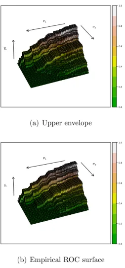
The lower and upper envelopes ROCLs(p1, p3) and ROC U
s(p1, p3) for the
set Sroc of all NPI-based ROC surfaces are presented in Figure 3, together
with the empirical ROC surface. In these plots, p1 and p3 increase from
0 to 1 in the directions indicated by arrows. The empirical ROC surface is everywhere between the two envelopes but the differences are small. The NPI lower and upper ROC surfaces, presented in Section 4.4, are not plotted, they are contained within the envelopes and differ only very little from them. The VUS values of the seven surfaces presented in this paper, so also in-cluding the further bounds in Section 4.6, are given in Table 1. They reflect
●
●
●
ADC NAS NEG
1.2 1.4 1.6 1.8 2.0 2.2 NAA/Cr le vels
Figure 2: Boxplots of NAA/Cr levels for the ADC, NAS and NEG groups
indeed that the differences between these surfaces are small. To interpret these values, it is important to remember that a VUS of about 1/6 occurs if the observations from the three groups fully overlap, in such a way that the diagnostic method would perform no better than a random allocation of patients to the three groups. As all VUS values are clearly greater than 1/6, this indicates that the diagnostic method is better than a random allo-cation. However, the VUS values are far away from 1, which would indicate perfect diagnostic performance. It is clear from Figure 2 that particularly the data from the NAS and NEG groups overlap substantially. These VUS values also imply that the NPI lower and upper ROC surfaces are close to the corresponding envelopes and that the upper bound for the NPI lower ROC surface and the lower bound for the NPI upper ROC surface are a bit further from the NPI lower and upper ROC surfaces than the corresponding envelopes. All bounds together could be useful if one would not have gone through the efforts of calculating the NPI lower and upper ROC surfaces exactly, as they would provide ranges within which the exact surfaces are.
P1 P3 Sf 0.0 0.2 0.4 0.6 0.8 1.0
(a) Upper envelope
P1 P3 Sf 0.0 0.2 0.4 0.6 0.8 1.0
(b) Empirical ROC surface
P1 P3 Sf 0.0 0.2 0.4 0.6 0.8 1.0 (c) Lower envelope
Table 1: Volumes under ROC surfaces [ V U S 0.2879 (V U SL, V U SU) (0.2524,0.3131) (V U S, V U S) (0.2548,0.3087) (V U SU, V U SL) (0.2688,0.2951)
ROC surface is equal to 1.4362, which occurs for (c1, c2) = (1.76,2.05). The
maximum values for the Youden’s indices corresponding to the NPI lower and upper ROC surfaces are J(c1, c2) = 1.3803 andJ(c1, c2) = 1.4732, which
both occur for the same values of c1 andc2 as for the empirical ROC surface.
These maximum values for the Youden’s indices indicate that the diagnostic performance of this test for the next patient is likely to be better than random classification, but it is not very good. With these optimal decision thresholds for diagnosis of the next patient, a test result less than or equal to 1.76 leads to classification into the ADC group, a test result greater than 2.05 leads to classification into the NEG group, and a rest result in between these two values leads to classification into the NAS group. The corresponding NPI lower and upper probabilities for correct classification are 0.6000 and 0.6167 for the next patient if from the ADC group, 0.6750 and 0.7250 if from the NAS group, and 0.1053 and 0.1316 if from the NEG group. The substantial overlap between the data from the NAS and NEG groups has resulted in an optimal classification method where nearly the entire range of values of this overlap leads to classification in the NAS group, which explains the small values of the NPI lower and upper probabilities for correct classification if the next patient is from the NEG group.
Coolen-Maturi et al. (2013) present two further examples, with smaller data sets and with less overlap between the data from the three groups. They illustrate some further aspects of this NPI approach, including that the difference between corresponding NPI upper and lower probabilities tends to be greater if there are fewer data observations and thus reflects the amount of information on which the inferences are based. Of course, if there is less overlap between the data from the three groups, the classification methods perform substantially better than in the example presented here.
6. Concluding remarks
In this paper we introduced the NPI approach for three-group diagnostic tests using the ROC surface. This can be used to asses the accuracy of a diagnostic test, with the NPI setting ensuring, due to its predictive nature, specific focus on the next patient. NPI lower probabilities reflect the evi-dence in favour of the event of interest, while NPI upper probabilities reflect the evidence against the event of interest. When making decisions about diagnosis for a specific future patient, it seems useful to have the amount of information and the evidence it provides clearly reflected in this way.
Attention has been restricted to real-valued data, developing the related NPI theory for ROC surfaces in case of ordinal data is an interesting topic for future research (Elkhafifi and Coolen, 2012; Coolen et al., 2013). The con-cepts and ideas presented can be generalized to classification into more than three categories (Waegeman et al., 2008), but the computation of NPI lower and upper ROC hypersurfaces, in line with Section 4.4, will require numerical optimisation which will be complicated for larger data sets with substantial overlap between observations from different groups. Generalization of the lower and upper envelopes of the set of all NPI-based ROC hypersurfaces is likely to remain feasible with more categories, but it has not yet been stud-ied in detail. Heuristic methods to approximate the NPI lower and upper ROC hypersurfaces may be required, the quality of such approximations, in relation to the computational complexity for their implementation, requires detailed study.
Development of NPI methods for ROC analysis including covariates is an important challenge (Lopez-de Ullibarri et al., 2008; Rodriguez-Alvarez et al., 2011a,b). Research of a general NPI approach for regression-type models is currently in progress. It is also possible to assume semi-parametric models in ROC analysis (Zhang, 2006; Wan and Zhang, 2008; Li and Zhou, 2009). Combining the NPI approach with partial parametric model assump-tions, which would also enable application to ROC problems, is an important topic for future research. Increasingly, statistical data are high-dimensional, which sets new challenges for analysis of diagnostic accuracy including ROC methods (Adler and Lausen, 2009). NPI has not yet been developed for multi-dimensional data, it is an important research challenge and may require additional structural model assumptions due to the curse of dimensionality that generally affects nonparametric methods.
assumed underlying population, but instead explicitly focuses on a future observation, it is quite different in nature to the established statistical ap-proaches, but in practice a predictive formulation may often be natural. NPI for real-valued observations is also available for multiple future observations (Arts et al., 2004; Coolen, 2011), where the inter-dependence of these future observations is explicitly taken into account. Development of NPI-based methods for diagnostic accuracy with explicit focus on m ≥ 2 future ob-servations is an interesting topic for future research, where particularly the strength of the inferences as function of m should be studied carefully, see Coolen and Coolen-Schrijner (2007) for a similar study with focus on the role of m for comparison of groups of Bernoulli data. Typically, for increasing m the imprecision in inferences increases, which is likely to imply that, on the basis of the limited information in available data, a specific choice of di-agnostic method including the important decision thresholds can be inferred to be good for a number of future patients up to a specific value of m, but for larger values of m the evidence in the data would be too weak to make decisions that are strongly supported by the data without further modelling assumptions.
We should emphasize that we do not advocate the NPI approach pre-sented here as a replacement of more established methods, but as an inter-esting alternative approach to important problems which we recommend to be used alongside other methods. If the results of different methods are quite close that provides a strong argument in favour of them, while substantial differences might suggest that further investigation would be beneficial. In particular, as most established statistical methods make stronger modelling assumptions, it would be logical in such cases to consider whether or not such assumptions are supported by the data.
There is a wide range of related topics which are of practical relevance but require further research. This includes dealing with continuous disease states which also need to be classified into groups (Shiu and Gatsonis, 2012), and the use of alternatives to the VUS (van Calster et al., 2012) or Youden’s index in such ROC-based analyses (Greiner et al., 2000; Schafer, 1989; Yousef et al., 2009; Lai et al., 2012). The possibility that the data may contain errors is also of great practical importance. All such topics provide interesting challenges for the further development and application of the NPI approach.
Acknowledgement
We are grateful to Dr. Christos Nakas for stimulating discussions about this topic area and for providing the data used in the example. We thank two reviewers whose detailed comments on an earlier version of this paper led to improved presentation.
Appendix A
In this paper, several volumes under surfaces have been presented. They are all proven following similar steps, which we present for Equation (7); they are all presented in detail by Coolen-Maturi et al. (2013). We use the notation
{A}+ = max{A,0} and P
p1
P
p3
to indicate the sum over pairs of values forp1
and p3 such that one value for p1 is taken from each interval (nix−+11 ,nxi+1)
for i = 1, . . . , nx + 1, and one value for p3 from each interval (nlz−+11 ,nzl+1)
for l = 1, . . . , nz + 1. As the considered ROC surfaces are constant for all
values p1 ∈ (nix−+11 ,nxi+1) and p3 ∈ (nlz−+11 ,nzl+1), it does not matter which
specific values for p1 and p3 within these intervals are actually used in the
calculations (e.g. mid-points of the intervals). Equation (7) is derived as follows. V U SL= 1 (nx+ 1)(nz + 1) X p1 X p3 ROCLs(p1, p3) = 1 (nx+ 1)(nz + 1) X p1 X p3 Fy(z(1−p 3))−Fy(x(p1)) + = 1 (nx+ 1)(nz + 1) nx+1 X i=1 nz+1 X l=1 Fy(zl−1)−Fy(xi) + =A nx+1 X i=1 nz+1 X l=1 (ny+1 X j=1 I(yj ≤zl−1)− ny+1 X j=1 I(yj−1 ≤xi) )+ =A nx+1 X i=1 ny+1 X j=1 nz+1 X l=1 I(yj ≤zl−1∧yj−1 > xi)
Appendix B
We present a proof for Theorem 4.3. For known probability distributions for the random quantities Xnx+1, Yny+1 and Znz+1,
P(Xnx+1 < Yny+1 < Znz+1) = nx+1 X i=1 ny+1 X j=1 nz+1 X l=1 P Xnx+1 < Yny+1 < Znz+1|Xnx+1 ∈(xi−1, xi), Yny+1 ∈(yj−1, yj), Znz+1 ∈(zl−1, zl)} ×P(Xnx+1 ∈(xi−1, xi))P(Yny+1 ∈(yj−1, yj))P(Znz+1 ∈(zl−1, zl))
This holds for all combinations of probability distributions for Xnx+1 in Px,
Yny+1 in Py and Znz+1 in Pz. We need to find the infimum and supremum
for this probability over all these combinations.
To derive the NPI lower probability for this event, the probability 1/(nx+
1) for Xnx+1, as assigned to each interval in the partition of the real-line
created by the observations from group Gx, is put at the right-end point of
each interval. Simultaneously, the probability 1/(nz+1) forZnz+1, as assigned
to each interval in the partition of the real-line created by the observations from group Gz, is put at the left-end point of each interval. This leads to
inf Px,Py,Pz P(Xnx+1 < Yny+1 < Znz+1) = 1 (nx+ 1)(nz+ 1) × inf Py nx+1 X i=1 ny+1 X j=1 nz+1 X l=1 P(xi < Yny+1 < zl−1|Yny+1 ∈(yj−1, yj))P(Yny+1 ∈(yj−1, yj)) (20) Here the infima are with regard to all probability distributions in the respec-tive structures.
By similar reasoning, the corresponding NPI upper probability requires the probability masses for Xnx+1 and Znz+1 to be put at the opposite end
points of the respective intervals. This leads to sup Px,Py,Pz P(Xnx+1 < Yny+1 < Znz+1) = 1 (nx+ 1)(nz+ 1) × sup Py nx+1 X i=1 ny+1 X j=1 nz+1 X l=1 P(xi−1 < Yny+1 < zl|Yny+1 ∈(yj−1, yj))P(Yny+1 ∈(yj−1, yj)) (21)
The remaining optimisation problems are how to assign the probability masses 1/(ny+ 1) forYny+1 within each interval (yj−1, yj),j = 1, . . . , ny+ 1,
for the NPI lower probability and for the NPI upper probability. Let the number of observations from groups Gx and Gz between yj−1 and yj be
denoted bynj
x andnjz, respectively. These observations partition the interval
(yj−1, yj) intonjx+njz+ 1 sub-intervals, the assumption that the data contain
no ties simplifies notation but can be relaxed without affecting the approach. If there are no observations from groups Gx andGz in the interval (yj−1, yj),
then the following reasoning still applies with this whole interval being the only ‘sub-interval’.
It is easy to see that this optimisation with regard to the probability distribution forYny+1can be achieved by putting the probability mass 1/(ny+
1) within an interval (yj−1, yj) in a single point, saytjmirelated to the infimum
and tj
ma related to the supremum. Doing this for all j = 1, . . . , ny+ 1, and
using the NPI lower and upper CDFs forXnx+1 and Znz+1, the optimisation
problem (20) is equivalent to inf 1 ny+ 1 ny+1 X j=1 Fx(tjmi)(1−Fz(t j mi))
and the optimisation problem (21) is equivalent to
sup 1 ny + 1 ny+1 X j=1 Fx(tjma)(1−Fz(t j ma))
where the infimum and supremum are with regard to the values tjmi and tjma over all possible sub-intervals of (yj−1, yj) for eachj ∈ {1, . . . , ny+ 1}. These
optimisations can be solved by minimising and maximising, respectively, the products within the sums on the right-hand sides. As these lower and upper CDFs are step-functions, these optimisations can be quite easily performed. However, these products are not monotone over the intervals (yj−1, yj), so
careful searches are required. This can be simplified using the knowledge that the CDFs are non-decreasing step-functions, and the fact that it is irrelevant which specific point within a sub-interval (as created by the x and z observations) is chosen. It is quite straightforward to implement an algorithm for these optimisations, one can take e.g. the mid-point of each sub-interval as candidate point to be tjmi or tj
Once these optimisations have been performed, we denote the points to which the probability masses for Yny+1 in the intervals (yj−1, yj) are assigned
bytjmin andtjmax,j = 1, . . . , ny+ 1, these are the points used in Theorem 4.3.
References
Adler, W., Lausen, B., 2009. Bootstrap estimated true and false positive rates and ROC curve. Computational Statistics & Data Analysis 53, 718–729. Airola, A., Pahikkala, T., Waegeman, W., De Baets, B., Salakoski, T., 2011.
An experimental comparison of cross-validation techniques for estimating the area under the ROC curve. Computational Statistics & Data Analysis 55, 1828–1844.
Arts, G.R.J., Coolen, F.P.A., van der Laan, P., 2004. Nonparametric pre-dictive inference in statistical process control. Quality Technology and Quantitative Management 1, 201–216.
Augustin, T., Coolen, F.P.A., 2004. Nonparametric predictive inference and interval probability. Journal of Statistical Planning and Inference 124, 251–272.
Beck, A.C., 2005. Receiver Operating Characteristic surfaces: Inference and Applications. Ph.D. thesis. University of Rochester. Rochester, New York. van Calster, B., van Belle, V., Vergouwe, Y., Steyerberg, E.W., 2012. Dis-crimination ability of prediction models for ordinal outcomes: Relation-ships between existing measures and a new measure. Biometrical Journal 54, 674–685.
Chang, L., Lee, P.L., Yiannoutsos, C.T., Ernst, T., Marra, C.M., Richards, T., Kolson, D., Schifitto, G., Jarvik, J.G., Miller, E.N., Lenkinski, R., Gonzalez, G., Navia, B.A., 2004. A multicenter in vivo proton-mrs study of hiv-associated dementia and its relationship to age. NeuroImage 23, 1336–1347.
Chen, W., Yousef, W., Gallas, B., Hsu, E., Lababidi, S., Tang, R., Pennello, G., Symmans, W., Pusztai, L., 2012. Uncertainty estimation with a finite dataset in the assessment of classification models. Computational Statistics & Data Analysis 56, 1016–1027.
Coolen, F.P.A., 2006. On nonparametric predictive inference and objective bayesianism. Journal of Logic, Language and Information 15, 21–47. Coolen, F.P.A., 2011. Nonparametric predictive inference, in: Lovric, M.
(Ed.), International Encyclopedia of Statistical Science. Springer, pp. 968– 970.
Coolen, F.P.A., Coolen-Schrijner, P., 2007. Nonparametric predictive com-parison of proportions. Journal of Statistical Planning and Inference 137, 23–33.
Coolen, F.P.A., Coolen-Schrijner, P., Coolen-Maturi, T., Elkhafifi, F.F., 2013. Nonparametric predictive inference for ordinal data. Communi-cations in Statistics - Theory and Methods to appear.
Coolen, F.P.A., Troffaes, M.C., Augustin, T., 2011. Imprecise probability, in: Lovric, M. (Ed.), International Encyclopedia of Statistical Science. Springer, pp. 645–648.
Coolen-Maturi, T., Coolen-Schrijner, P., Coolen, F.P.A., 2012a. Nonpara-metric predictive inference for binary diagnostic tests. Journal of Statistical Theory and Practice 6, 665–680.
Coolen-Maturi, T., Coolen-Schrijner, P., Coolen, F.P.A., 2012b. Nonpara-metric predictive inference for diagnostic accuracy. Journal of Statistical Planning and Inference 142, 1141–1150.
Coolen-Maturi, T., Elkhafifi, F.F., Coolen, F.P.A., 2013. Nonparamet-ric predictive inference for three-group ROC analysis. Technical Report (www.npi-statistics.com).
De Finetti, B., 1974. Theory of Probability. Wiley, London.
Elkhafifi, F.F., Coolen, F.P.A., 2012. Nonparametric predictive inference for accuracy of ordinal diagnostic tests. Journal of Statistical Theory and Practice 6, 681–697.
Greiner, M., Pfeiffer, D., Smith, R.D., 2000. Principles and practical appli-cation of the receiver-operating characteristic analysis for diagnostic tests. Preventive Veterinary Medicine 45, 23–41.
Heckerling, P.S., 2001. Parametric three-way receiver operating characteristic surface analyis using Mathematica. Medical Decision Making 20, 409–417. Hill, B.M., 1968. Posterior distribution of percentiles: Bayes’ theorem for sampling from a population. Journal of the American Statistical Associa-tion 63, 677–691.
Inacio, V., Turkman, A.A., Nakas, C.T., Alonzo, T.A., 2011. Nonparametric Bayesian estimation of the the three-way receiver operating characteristic surface. Biometrical Journal 53, 1011–1024.
Lai, C., Tian, L., Schisterman, E., 2012. Exact confidence interval estimation for the youden index and its corresponding optimal cut-point. Computa-tional Statistics & Data Analysis 56, 1103–1114.
Lawless, J.F., Fredette, M., 2005. Frequentist prediction intervals and pre-dictive distributions. Biometrika 92, 529–542.
Li, J., Zhou, X.H., 2009. Nonparametric and semiparametric estimation of the three way receiver operating characteristic surface. Journal of Statis-tical Planning and Inference 139, 4133–4142.
Lopez-de Ullibarri, I., Cao, R., Cadarso-Suarez, C., Lado, M., 2008. Nonpara-metric estimation of conditional ROC curves: Application to discrimina-tion tasks in computerized detecdiscrimina-tion of early breast cancer. Computadiscrimina-tional Statistics & Data Analysis 52, 2623–2631.
Mossman, D., 1999. Three-way rocs. Medical Decision Making 19, 78–89. Nakas, C.T., Alonzo, T.A., 2007. ROC graphs for assessing the ability of a
diagnostic marker to detect three disease classes with an umbrella ordering. Biometrics 63, 603–609.
Nakas, C.T., Alonzo, T.A., Yiannoutsos, C.T., 2010. Accuracy and cut-off point selection in three-class classification problems using a generalization of the youden index. Statistics in Medicine 29, 2946–2955.
Nakas, C.T., Yiannoutsos, C.T., 2004. Ordered multiple-class ROC analysis with continuous measurements. Statistics in Medicine 23, 3437–3449.
Nakas, C.T., Yiannoutsos, C.T., 2010. Ordered multiple class receiver oper-ating characteristic (ROC) analysis, in: Chow, S.C. (Ed.), Encyclopedia of Biopharmaceutical Statistics. Informa Healthcare, pp. 929–932.
Pepe, M.S., 2003. The Statistical Evaluation of Medical Tests for Classifica-tion and PredicClassifica-tion. Oxford University Press, Oxford.
Rodriguez-Alvarez, M., Roca-Pardinas, J., Cadarso-Suarez, C., 2011a. A new flexible direct ROC regression model: Application to the detection of cardiovascular risk factors by anthropometric measures. Computational Statistics & Data Analysis 55, 3257–3270.
Rodriguez-Alvarez, M., Tahoces, P., Cadarso-Suarez, C., Lado, M., 2011b. Comparative study of ROC regression techniques - applications for the computer-aided diagnostic system in breast cancer detection. Computa-tional Statistics & Data Analysis 55, 888–902.
Schafer, H., 1989. Constructing a cut-off point for a quantitative diagnostic test. Statistics in Medicine 8, 1381–1391.
Shiu, S.Y., Gatsonis, C., 2012. On ROC analysis with nonbinary reference standard. Biometrical Journal 54, 457–480.
Tian, L., Xiong, C., Lai, Y., Vexler, A., 2011. Exact confidence interval es-timation for the difference in diagnostic accuracy with three ordinal diag-nostic groups. Journal of Statistical Planning and Inference 141, 549–558. Waegeman, W., De Baets, B., Boullart, L., 2008. On the scalability of ordered multi-class ROC analysis. Computational Statistics & Data Analysis 52, 3371–3388.
Walley, P., 1991. Statistical Reasoning with Imprecise Probabilities. Chap-man & Hall, London.
Wan, S., Zhang, B., 2008. Comparing correlated ROC curves for continuous diagnostic tests under density ratio models. Computational Statistics & Data Analysis 52, 233–245.
Weichselberger, K., 2000. The theory of interval-probability as a unifying concept for uncertainty. International Journal of Approximate Reasoning 24, 149–170.
Weichselberger, K., 2001. Elementare Grundbegriffe einer allgemeineren Wahrscheinlichkeitsrechnung I. Intervallwahrscheinlichkeit als umfassendes Konzept. Physica, Heidelberg.
Wians, F.H.J., Urban, J.E., Keffer, J.H., Kroft, S.H., 2001. Discriminating between iron deficiency anemia and anemia of chronic disease using tradi-tional indices of iron status vs transferrin receptor concentration. American Journal of Clinical Pathology 115, 112–118.
Xanthopoulos, S.Z., Nakas, C.T., 2007. A generalized ROC approach for the validation of credit rating systems and scorecards. The Journal of Risk Finance 8, 481 – 488.
Xiong, C., van Belle, G., Miller, J.P., Yan, Y., Gao, F., Yu, K., Morris, J.C., 2007. A parametric comparison of diagnostic accuracy with three ordinal diagnostic groups. Biometrical Journal 49, 682–693.
Yiannoutsos, C.T., Nakas, C.T., Navia, B.A., 2008. Assessing multiple-group diagnostic problems with multi-dimensional receiver operating character-istic surfaces: Application to proton mr spectroscopy (mrs) in hiv-related neurological injury. Neuroimage 40, 248–255.
Youden, W.J., 1950. Index for rating diagnostic tests. Cancer 3, 32–35. Yousef, W., Kundu, S., Wagner, R., 2009. Nonparametric estimation of
the threshold at an operating point on the ROC curve. Computational Statistics & Data Analysis 53, 4370–4383.
Zhang, B., 2006. A semiparametric hypothesis testing procedure for the ROC curve area under a density ratio model. Computational Statistics & Data Analysis 50, 1855–1876.
Zhou, X.H., Obuchowski, N.A., McClish, D.K., 2011. Statistical Methods in Diagnostic Medicine. Wiley, New York.
Zou, K.H., Liu, A., Bandos, A.I., Ohno-Machado, L., Rockette, H.E., 2011. Statistical Evaluation of Diagnostic Performance: Topics in ROC Analysis. Chapman Hall / CRC, Boca Raton.