and Its Application for Reachability Analysis
Orna Grumberg, Assaf Schuster, and Avi YadgarComputer Science Department, Technion, Haifa, Israel
Abstract. This work presents a memory-efficient All-SAT engine which, given a
propositional formula over sets of important and non-important variables, returns the set of all the assignments to the important variables, which can be extended to solutions (satisfying assignments) to the formula. The engine is built using elements of modern SAT solvers, including a scheme for learning conflict clauses and non-chronological backtracking. Re-discovering solutions that were already found is avoided by the search algorithm itself, rather than by adding blocking clauses. As a result, the space requirements of a solved instance do not increase when solutions are found. Finding the next solution is as efficient as finding the first one, making it possible to solve instances for which the number of solutions is larger than the size of the main memory.
We show how to exploit our All-SAT engine for performing image computation and use it as a basic block in achieving full reachability which is purely SAT-based (no BDDs involved).
We implemented our All-SAT solver and reachability algorithm using the state-of-the-art SAT solver Chaff [19] as a code base. The results show that our new scheme significantly outperforms All-SAT algorithms that use blocking clauses, as measured by the execution time, the memory requirement, and the number of steps performed by the reachability analysis.
1
Introduction
This work presents a memory-efficient All-SAT engine which, given a propositional for-mula over sets of important and non-important variables, returns the set of all the as-signments to the important variables, which can be extended to solutions (satisfying assignments) to the formula. The All-SAT problem has numerous applications in AI [21] and logic minimization [22]. Moreover, many applications require the ability to instantiate all the solutions of a formula, which differ in the assignment to only a subset of the variables. In [14] such a procedure is used for predicate abstraction. In [7] it is used for re-parameterization in symbolic simulation. In [18, 6] it is used for reachability analysis, and in [13] it is used for pre-image computation. Also, solving QBF is actually solving such a problem, as shown in [15].
Most modern SAT solvers implement the DPLL[9, 8] backtrack search. These sol-vers add clauses to the formula in order to block searching in subspaces that are known to contain no solution. All-SAT engines that are built on top of modern SAT solvers tend to extend this method by using additional clauses, called blocking clauses, to block solutions that were already found [18, 6, 13, 14, 7, 20]. However, while the addition of A.J. Hu and A.K. Martin (Eds.): FMCAD 2004, LNCS 3312, pp. 275–289, 2004.
c
blocking clauses prevents repetitions in solution creation, it also significantly inflates the size of the solved formula. Thus, the engine slows down corresponding to the num-ber of solutions that were already found. Eventually, if too many solutions exist, the engine may saturate the available memory and come to a stop.
In [6] an optimization is employed to the above method. The number of blocking clauses and the run time are reduced significantly by inferring from a newly found solu-tion a set of related solusolu-tions, and blocking them all with a single clause. This, however, is insufficient when larger instances are considered. Moreover, the optimization is ap-plicable only for formulae which originated from a model.
In this work we propose an efficient All-SAT engine which does not use blocking clauses. Given a propositional formula and sets of important and non-important vari-ables, our engine returns the set of all the assignments to the important varivari-ables, which can be extended to solutions to the formula. Setting the non-important variables set to be empty, yields all the solutions to the formula. Similar to previous works, our All-SAT solver is also built on top of a SAT solver. However, in order to block known solutions, it manipulates the backtracking scheme and the representation of the implication graph. As a result, the size of the solved formula does not increase when solutions are found. Moreover, since found solutions are not needed in the solver, they can be stored in ex-ternal memory (disk or the memory of another computer), processed and even deleted. This saving in memory is a great advantage and enables us to handle very large instances with huge number of solutions. The memory reduction also implies time speedup, since the solver handles much less clauses. In spite of the changes we impose on backtrack-ing and the implication graph, we manage to apply many of the operations that made modern SAT solvers so efficient. We derive conflict clauses based on conflict analysis, apply non-chronological backtracking to skip subspaces which contain no solutions, and apply conflict driven backtracking under some restrictions.
We show how to exploit our All-SAT engine for reachability analysis, which is an important component of model checking. Reachability analysis is often used as a preprocessing step before checking. Moreover, model checking of most safety tempo-ral properties can be reduced to reachability analysis [1]. BDD-based algorithms for reachability are efficient when the BDDs representing the transition relation and the set of model states can be stored in memory [4, 5]. However, BDDs are quite unpredictable and tend to explode on intermediate results of image computation. When using BDDs, a great effort is invested in finding the optimal variables order. SAT-based algorithms, on the other hand, can handle models with larger number of variables. However, they are mainly used for Bounded Model Checking (BMC) [2].
Pure SAT-based methods for reachability [18, 6] and model checking of safety prop-erties [13, 20] are based on All-SAT engines, which return the set of all the solutions to a given formula. The All-SAT engine receives as input a propositional formula describ-ing the application of a transition relationT to a set of statesS. The resulting set of solutions represents the image ofS(the set of all successors for states inS). Repeating this step, starting from the initial states, results in the set of all reachable states.
Similar to [18, 6], we exploit our All-SAT procedure for computing an image for a set of states, and then use it iteratively for obtaining full reachability. Several optimiza-tions are applied at that stage. Their goals are to reduce the number of found soluoptimiza-tions
by avoiding repetitions between images; to hold the found solutions compactly; and to keep the solved formula small.
An important observation is that for image computation, the solved formula is de-fined over variables describing current statesx, inputsI, next statesx, and some aux-iliary variables that are added while transforming the formula to CNF. However, many solutions to the formula are not needed: the only useful ones are those which give dif-ferent values tox. This set of solutions is efficiently instantiated by our algorithm by definingxas the important variables. Since the variables inxtypically constitute just 10% of all the variables in the formula [23], the number of solutions we search for, produce, and store, is reduced dramatically. This was also done in [18, 6, 13, 20].
Other works also applied optimizations within a single image [6] and between im-ages [18, 6]. These have similar strength to the optimization we apply between imim-ages. However, within an image computation we gain significant reductions in memory and time due to our new All-SAT procedure, and the ability to process the solutions outside the engine before the completion of the search. This gain is extended to the reachability computation as well, as demonstrated by our experimental results.
In [11], a hybrid of SAT and BDD methods is proposed for image computation. This implementation of an All-SAT solver does not use blocking clauses. The known solutions are kept in a BDD which is used to restrict the search space of the All-SAT engine. While this representation might be more compact than blocking clauses, the All-SAT engine still depends on the set of known solutions when searching for new ones. Moreover, since our algorithm does not impose restrictions on learning, we believe it can be used to enhance the performance of such hybrid methods as well.
In [3, 12] all the solutions of a given propositional formula are found by repeatedly choosing a value to one variable, and splitting the formula accordingly, until all the clauses are satisfied. However, in this method, all the solutions of the formula are found, while many of them represent the same next state. Therefore, it can not be efficiently applied for quantifier elimination and image computation.
We have built an All-SAT solver based on the state-of-the-art SAT solver Chaff [19]. Experimental results show that our All-SAT algorithm outperforms All-SAT algorithms based on blocking clauses. Even when discovering a huge number of solutions, our solver does not run out of memory, and does not slow down. Similarly, our All-SAT reachability algorithm also achieves significant speedups over blocking clauses-based All-SAT reachability, and succeeds to perform more image steps.
The rest of the paper is organized as follows. Section 2 gives the background needed for this work. Sections 3 and 4 describe our algorithm and its implementation. Section 5 describes the utilization of our algorithm for reachability analysis. Section 6 shows our experimental results, and Section 7 includes conclusions.
2
Background
2.1 The SAT Problem
The Boolean satisfiability problem (SAT) is the problem of finding an assignmentA to a set of Boolean variablesV such that a Boolean formulaφ(V)will have the value ‘true’ under this assignment. A is called a satisfying assignment, or a solution, forφ.
We shall discuss formulae presented in the conjunctive normal form (CNF). That is,φis a conjunction of clauses, while each clause is a disjunction of literals overV. A literallis an instance of a variable or its negation:l ∈ {v,¬v | v ∈ V}. We shall consider a clause as a set of literals, and a formula as a set of clauses.
A clausecl is satisfied under an assignmentA iff ∃l ∈ cl, A(l) = true. For a formulaφgiven in CNF, an assignment satisfiesφiff it satisfies all of its clauses. Hence, if, under an assignmentA(or a partial assignment), all of the literals of some clause in φare false, thanAdoes not satisfyφ. We call this situation a conflict.
2.2 Davis-Putnam-Logemann-Loveland Backtrack Search (DPLL)
We begin by describing the Boolean Constraint Propagation (bcp()) procedure. Given a partial assignmentAand a clausecl, if there is one literall∈clwith no value, while the rest of the literals are all false, then in order to avoid a conflict,Amust be extended such thatA(l) =true.clis called a unit clause or an asserting clause, and the assignment tolis called an implication. The bcp() procedure finds all the implications at a given moment. This procedure is efficiently implemented in [19, 10, 26, 17, 16].
The DPLL algorithm [9, 8] walks the binary tree that describes the variables space. At each step, a decision is made. That is, a value to one of the variables is chosen, thus reaching deeper in the tree. Each decision is assigned with a new decision level. After a decision is made, the algorithm uses the bcp() procedure to compute all its implications. All the implications are assigned with the corresponding decision level. If a conflict is reached, the algorithm backtracks in the tree, and chooses a new value to the most recent variable not yet tried both ways. The algorithm terminates if one of the leaves is reached with no conflict, describing a satisfying assignment, or if the whole tree was searched and no satisfying assignment was found, meaningφis unsatisfiable.
2.3 Optimizations
Current state of the art SAT solvers use Conflict Analysis, Learning, and Conflict Driven
Backtracking to optimize the DPLL algorithm [27, 17]. Upon an occurrence of a
con-flict, the solver creates a conflict clause which implies the reverse assignment to some variable in the highest level. This clause is added to the formula to prune the search tree [27, 17]. In order to emphasize the recently gained knowledge, the solver uses
con-flict driven backtracking: Letlbe the highest level of an assigned variable in the conflict clause. The solver discards some of its work by invalidating all the assignments abovel. The implication of the conflict clause is then added tol[27]. This implies a new order of the variables in the search tree. Note that the other variables for which the assignments were invalidated, may still assume their original values, and lead to a solution.
Next we describe the implication graph, which is used to create conflict clauses. An
Implication Graph represents the current partial assignment during the solving process,
and the reason for the assignment to each variable. For a given assignment, the implica-tion graph is not unique, and depends on the decisions and the order used by the bcp(). We denote the asserting clause that implied the value oflbyante(l), and refer to it as the antecedent ofl. Iflis a decision,ante(l) =NULL. Given a partial assignmentA:
– The implication graph is a directed acyclic graphG(L, E).
– The vertices are the literals of the current partial assignment:∀l ∈L, l∈ {v,¬v | v∈V ∧A(l) =true}.
– The edges are the reasons for the assignments:E = (li, lj) | li, lj ∈ L, li ∈ ante(lj). That is, for each vertexl, the incident edges represent the clauseante(l). A decision vertex has no incident edge.
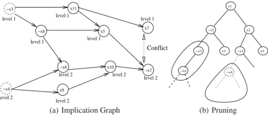
– Each vertex is also assigned with the decision level of the corresponding variable. When a conflict occurs, there are both true and false vertices of some variable, denoted conflicting variable. A Unique Implication Point (UIP) in an implication graph is a vertex of the current decision level, through which all the paths from the decision vertex of this level to the conflict pass. There may be more than one UIP, and we order them starting from the conflict. The decision variable of a level is always a UIP. When conflict driven backtracking is used, the conflict analysis creates a conflict clause which is a unit clause. This clause implies the reverse assignment to one of the UIPs. After backtracking, the opposite value of the UIP becomes an implication, and the conflict clause is its antecedent [27]. Figure 1(a,b) shows an implication graph with a conflict and two UIPs, and the pruning of the search tree by a conflict clause.
Conflict level 1 level 2 level 1 level 1 level 1 level 2 level 2 level 2 level 2 level 1 x11 −x6 −x7 −x3 x5 x7 −x8 x9 x10 −x4
(a) Implication Graph
−x3 x3 x1 −x3 −x2 x2 −x4 x3 −x4 (b) Pruning
Fig. 1. (a) An implication graph describing a conflict. The roots are decisions.¬x4 andx10are UIPs. (b) Adding the clause(x3, x4)prunes the search tree of the subspace defined by¬x3∧¬x4.
2.4 The All-SAT Problem
Given a Boolean formula presented in CNF, we would like to find all of its solutions as defined in the SAT problem.
The Blocking Clauses Method: A straight forward method to find all of the formula’s solutions is to modify the DPLL SAT solving algorithm such that when a solution is found, a blocking clause describing its negation is added to the solver, thus preventing the solver from reaching the same solution again. The last decision is then invalidated, and the search is continued normally. Once all of the solutions are found, there will be no satisfying assignment to the current formula, and the algorithm will terminate.
This algorithm suffers from exponential space growth as it adds a clause at the size ofV for each solution found. Another problem is that the increasing number of
clauses in the system will slow down the bcp() procedure which will have to look for implications in an increasing number of clauses.
3
Memory Efficient All-SAT Algorithm
3.1 ConventionsAssume we are given a partition of the variables to important and non-important vari-ables. Two solutions to the problem which differ in the non-important variables only are considered the same solution. Thus, a solution is defined by a subset of the variables.
A subspace of assignments, defined by a partial assignmentσ, is the set of all assign-ments which agree withσon its assigned variables. A subspace is called exhausted if all of the satisfying assignments in it (if any) were already found. At any given moment, the current partial assignment defines the subspace which is now being investigated.
We now present our All-SAT algorithm. A proof of its correctness is given in [25]. 3.2 The All-SAT Algorithm
Our algorithm walks the search tree of the important variables. We call this tree the
im-portant space. Each leaf of this tree represents an assignment to the imim-portant variables
which does not conflict with the formula. When reaching such a leaf, the algorithm tries to extend the assignment over the non-important variables. Hence, it looks for a solu-tion within the subspace defined by the important variables. Note that the walk over the
important space should be exhaustive, while only one solution for the non-important
variables should be found. This search is illustrated in Figure 2(a).
We incorporate these two behaviors into one procedure by modifying the decision and backtracking procedures of a conflict driven backtrack search, and the representa-tion of the implicarepresenta-tion graph.
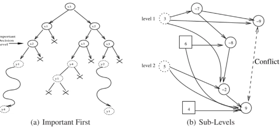
Important First Decision Procedure: We create a new decision procedure which looks for an unassigned variable from within the important variables. If no such variable is found, the usual decision procedure is used to choose a variable from the non-important set. This way, at any given time, the decision variables are a sequence of important variables, followed by a sequence of non important variables. At any given time, the
important decision level is the maximal level in which an important variable is a
deci-sion. An example is given in Figure 2(a).
Exhaustive Walk of the Important Space: An exhaustive walk of the important space is performed by extending the original DPLL algorithm with the following procedures: Chronological backtracking after a leaf of the important space is handled; Learning a conflict clause and chronological backtracking upon an occurrence of a conflict; Non-chronological backtracking when a subspace of the problem is proved to be exhausted. Chronological backtracking, as in DPLL, is done by flipping the highest important decision variable not yet flipped. This means that under the previous decisions, the last decision variable must assume the reverse assignment. Hence, its new value is an implication of the previous decisions. Therefore, in order to perform a chronological backtrack, we flip the highest decision and assign it with the level below. This way,
y1 y2 y4 y1 Important Level Decision x2 x3 x3 x2 x1 x3 y1 y4
(a) Important First
Conflict level 1 6 4 level 2 3 5 −7 9 −2 −8 −9 (b) Sub-Levels
Fig. 2. (a) Important First Decision.xvariables are important andyare non-importnat. (b) An implication graph in the presence of flipped decisions.6and4define new sub-levels.
the highest decision is always the highest decision not yet flipped. Higher decisions which were already flipped are regarded as its implications. Note, though, that there is no clause implying the values of the flipped decisions. Therefore, a new definition for the implication graph is required.
We change the definition of the implication graph as follows: Root vertices in the graph still represent the decisions, but also decisions flipped because of previous chronological backtracking. Thus, for conflict analysis purposes, a flipped decision is considered as defining a new decision sub-level. The result is a graph in which the nodes represent actual assignments to the variables, and the edges represent real clauses, mak-ing it a valid implication graph. This graph describes the current assignment, though not the current decisions. An example for such a graph is given in Figure 2(b).
Given the modified graph, the regular conflict analysis is performed, and leads to a UIP in the newly defined sub-level. The generated conflict clause is added to the formula to prune the search tree, as for solving the SAT problem. Modifying the impli-cation graph and introducing the new sub-levels may cause the conflict clause not to be asserting. However, since we do not use conflict driven backtracking in the important
space, our solver does not require that the conflict clauses will be asserting.
We now consider the case in which a conflict clause is asserting. In this case, we extend the current assignment according to it. Let c1 be a conflict clause, andlit its implication. Addinglitto the current assignment may cause a second conflict, for which litis the reason. Therefore, we are able to perform conflict analysis again, usinglitas a UIP. The result is a second conflict clause,c2which implies¬lit. It is obvious now that neither of the assignments tolitwill resolve the current conflict. The conclusion is that the reason for this situation lies in a lower decision level, and that a larger subspace is exhausted. We calculate c3 ← resolution(c1, c2) [9] and resolve the conflict by backtracking to the decision level preceding the highest level of a variable inc3, which is the level below the highest decision level of a variable inc1orc2. Note that backtracking to any level higher than that would not resolve the conflict as bothc1andc2would imply litand¬litrespectively. Therefore, by this non-chronological backtracking, we skip a large exhausted subspace.
Assigning Non-important Variables: After reaching a leaf in the important space, we have to extend the assignment to the non important variables. At this point, all the important variables are assigned with some value. Note, that since we only need one extension, we actually have to solve the SAT problem for the given formula with the current partial assignment. This is done by allowing the normal work of the optimized SAT algorithm, including decisions, conflict clause learning, and conflict driven back-tracking. However, we allow backtracking down to the important decision level but not below it, in order not to change the assignment to the important variables. If no solution is found, the current assignment to the important variables can not be extended to a solution for the formula, and should be discarded. On the other hand, if a solution to the formula is found, its projection over the important variables is a valid output. In both cases, we backtrack to the important decision level and continue the exhaustive walk of the important space.
4
Implementation
We implemented our All-SAT engine using zChaff [19] as a base code. This SAT solver uses the VSIDS decision heuristic [19], an efficient bcp() procedure, conflict clause learning, and conflict driven backtracking. We modified the decision procedure to match our important-first decision procedure, and added a mechanism for chronological back-tracking. We implemented the exhaustive walk over the important space using chrono-logical backtracking, and by allowing non-chronochrono-logical backtracking when subspaces without solutions are detected. We used the original optimized SAT solving procedures above the important decision level, where it had to solve a SAT problem. Next, we describe the modifications imposed on the solver in the important space.
The original SAT engine represents the current implication graph by means of an
assignment stack, hereafter referred to as stack. The stack consists of levels of
assign-ments. The first assignment in each level is the decision, and the rest of the assignments in the level are its implications. Each implication is in the lowest level where it is im-plied. Thus, an implication is implied by some of the assignments prior to it, out of which at least one is of the same level. For each assigned variable, the stack holds its value and its antecedent, where the antecedent of a decision variable is NULL.
In the following discussion, backtrack to levelirefers to the following procedure: a) Flipping the decision in leveli+ 1. b) Invalidation of all the assignments in levels i+ 1and above, by popping them out of the stack. c) Pushing the flipped decision at the end of leveli, with NULL antecedent. d) Executing bcp() to calculate the implications of the flipped decision.
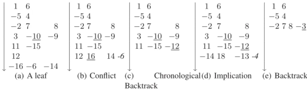
We perform chronological backtracking from leveljwithin the important space by backtracking to levelj−1. This way, the flipped decisions appear as implications of prior ones, and the highest decision not yet flipped is always the highest in the stack. The assignments with NULL antecedents, which represent exhausted subspaces, remain in the stack until a whole subspace which includes them is exhausted. An example for this procedure is given in Figure 3(a,b).
Our stack now includes decision variables, implications, and flipped decisions, which appear as implications but with no antecedents. Using this stack we can
con- 1 6 −5 4 −2 7 8 3 −10 −9 11 −15 12 −16−6 −14 (a) A leaf 1 6 −5 4 −2 7 8 3 −10−9 11 −15 12 16 14-6 (b) Conflict 1 6 −5 4 −2 7 8 3 −10 −9 11 −15−12 (c) Chronological Backtrack 1 6 −5 4 −2 7 8 3 −10 −9 11 −15−12 −14 18 −13-4 (d) Implication 1 6 −5 4 −2 7 8−3 (e) Backtrack
Fig. 3. Important Space Resolve Conflict (a) Reaching a leaf of the important space. ‘−10’ has NULL antecedent (b) Chronological backtrack which causes a conflict. ‘16’ has NULL antecedent, clausec1 = (−1,2,−14) is generated. (c) Chronological backtrack. (d) ‘−14’, the implication of clause c1, is pushed into the stack, and leads to a conflict. Clause c2 = (−4,2,−3,14)is generated.c3 ← resolution(c1, c2) = (−1,2,−3,−4). (e) Backtracking to the highest level inc3.
struct the implication graph according to the new definition given in section 3.2. Thus we can derive a conflict clause whenever a conflict occurs.
Decisions about exhausted subspaces are made during the process of resolving a conflict, as described next. We define a generated clauses stack, which is used to tem-porarily store clauses that are generated during conflict analysis1. In the following ex-planation, refer to Figure 3(b-e). (b) When a conflict occurs, we analyze it and learn a new conflict clause according to the 1UIP scheme [27]. This clause is added to the solver to prune the search tree, and is also pushed into the generated clauses stack to be used later. (c) We perform a chronological backtrack. A pseudo code for this pro-cedure is shown in Figure 4(‘chronological backtrack’). If this caused another conflict, we start the resolving process again. Otherwise, we start calculating the implications of the clauses in the generated clauses stack.
(d) Letc1be a clause popped out of the generated clauses stack. Ifc1 is not as-serting, we ignore it. If it implies lit, we push lit into the stack and run bcp(). For simplicity of presentation,lit is pushed to a new level in the stack. If a new conflict is found, we follow the procedure described in Section 3.2 to decide about exhausted subspaces. We create a new conflict clause,c2, withlitas the UIP.c1andc2implylit and¬litrespectively. We calculatec3 ←resolution(c1, c2)[9]. (e) We backtrack to the level preceding the highest level of an assigned variable inc3. Thus, we backtrack higher, skipping a large exhausted subspace. A pseudo code of this procedure is given in Figure 4.
5
Reachability and Model Checking Using All Solution Solver
5.1 ReachabilityWe now present one application of our All-SAT algorithm. Given the set of initial states of a model, and the transition relation, we would like to find the set of all the states
1
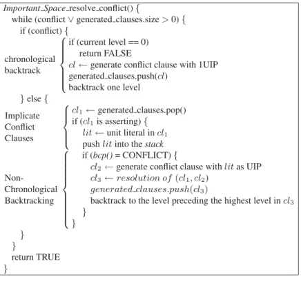
Important Space resolve conflict(){
while (conflict∨generated clauses.size>0){ if (conflict){ chronological backtrack if (current level == 0) return FALSE
cl←generate conflict clause with 1UIP generated clauses.push(cl)
backtrack one level
}else{ Implicate Conflict Clauses cl1←generated clauses.pop() if (cl1is asserting){
lit←unit literal incl1 pushlitinto the stack
Non-Chronological Backtracking if (bcp() = CONFLICT){
cl2←generate conflict clause withlitas UIP
cl3←resolution of(cl1, cl2)
generated clauses.push(cl3)
backtrack to the level preceding the highest level incl3
} } } } return TRUE }
Fig. 4. Important Space resolve conflict.
reachable from the initial states. We denote byxthe vector of the model state variables, and bySi(x)the set of states at distanceifrom the initial states. The transition relation is given byT(x, I, x)wherexrepresents the current state,Irepresents the input and x represents the next state. For a given set of statesS(x), the set of reachable states from them at distance 1 (i.e., their successors), denoted Image(S(x)), is
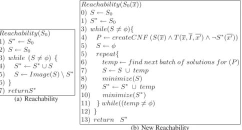
Image(S(x)) ={x | ∃x,∃I, S(x)∧T(x, I, x)} (1) GivenS0, the set of initial states, calculating the reachable states is done by iteratively calculatingSi, and adding them to the reachable setS∗, untilSicontains no new states. The rechability algorithm is shown in Figure 5(a).
5.2 Image Computation Using All-SAT
We would like to use our All-SAT algorithm in order to implement line 5 in the reach-ability algorithm (Figure 5(a)). In order to do that, we have to find all of the solutions for the following formula:
S(x)∧T(x, I, x)∧ ¬S∗(x) (2)
Each solution to (2) represents a valid transition from one of the states in the set S(x)to a new statex, which is not inS∗(x). Including¬S∗(x)in the image compu-tation was also done in [6, 18].
We now have to construct a CNF representation for Formula 2. We represent each statexas the conjunction of its literals. Therefore,S∗(x)is in DNF, and¬S∗(x)is in CNF. Creating the CNF representation forSis done by introducing auxiliary variables. The translations of both sets are linear in the size of the sets. Representing T as a CNF is also possible by introducing auxiliary variables [2].
Each solution is an assignment to all of the variables in the CNF, and its projection overx defines the new state. We avoid repetitive finding of the samexby settingx to be the important variables in our All-SAT solver. A state is found once, regardless of its predecessors, input, or the assignment to the auxiliary variables added during the CNF construction. Making the decisions from within the model variables proved to be efficient when solving SAT problems for BMC [23].
5.3 Minimization
Boolean Minimization: A major drawback of the implementation described above is the growth ofS∗ between iterations of the algorithm, and ofSduring the image com-putation. This poses a problem even when the solutions are held outside the solver. Representing each state by a conjunction of literals is pricey when their number in-creases. Therefore we need a way to minimize this representation. We exploit the fact that a set of states is actually a DNF formula and apply Boolean minimization methods to find a minimal representation for this formula. For example, the solutions represented by(x0∧x1)∨(x0∧ ¬x1), can be represented by(x0).
In our tool, we use Berkeley’s ‘Espresso’[24], which receives as an input a set of DNF clauses and returns their minimized DNF representation. Our experimental results show a reduction of up to 3 orders of magnitude in the number of clauses required to represent the sets of solutions when using this tool.
On-the-Fly Minimization: Finding all the solutions for Formula (2), and then mini-mizing them, is not feasible for large problems since their number would be too large to store and for the minimizer to handle. Therefore, during the solving process, when-ever a preset number of solutions is found, the solver work is suspended, and we use the minimizer to combine them with the currentSandS∗. The output, then, is stored again inSandS∗respectively, to be processed with the next batch of solutions found by the All-SAT solver. This way, we keepS∗,S and the input to the minimizer small. Note, also, that each batch of solutions includes new states only, due to the structure of Formula 2. Employing logical minimization on-the-fly, before finding all the solu-tions, is possible since previous solutions are not required when searching for the next ones, and the work of the minimizer is independent of the All-SAT solver. Moreover, the minimization and the computation of the next batch of solutions can be performed concurrently. However, this is not implemented in our tool. Note, that this minimization does not effect the performance of the All-SAT solver.
We now have a slightly modified reachability algorithm as shown in Figure 5(b).
6
Experimental Results
As the code base for our work, we use the zChaff SAT solver [19] which is one of the fastest available state of the art solvers. zChaff implements conflict analysis with
Reachability(S0) 1) S∗←S0 2) S←S0 3) while (S=φ) { 4) S∗←S∗∪S 5) S←Image(S)\S∗ 6) } 7) returnS∗ (a) Reachability Reachability(S0(x)) 0) S←S0 1) S∗←S0 3) while(S=φ){ 4) P ←createCN F(S(x)∧T(x, I, x)∧ ¬S∗(x)) 5) S←φ 5) repeat{
6) temp←f ind next batch of solutions f or(P)
7) S←S ∪ temp 8) minimize(S) 9) S∗←S∗ ∪ temp 10) minimize(S∗) 11) }while((temp=φ) 12) } 13) return S∗ (b) New Reachability
Fig. 5. Reachability Algorithms. (a) Regular reachability algorithm. (b) Reachability using out
All-SAT solver. Lines 5-11 are the implementation of the on-the-fly minimization.
conflict driven backtrack, and uses efficient data structures. Since zChaff is open source, we were able to modify the code according to our method.
For comparison, we used the same code base to implement the blocking clauses method. In order to avoid repetition of the same assignments to the important variables, we constructed the blocking clauses from the important variables only. We improved the blocking clauses by using the decision method described in Section 3.2. This way, the blocking clauses can be constructed from only the subset of the important variables which are decision variables, since the rest of the assignments are implied by them. This improvement reduced space requirements as well as solution times of the blocking clauses method substantially.
All experiments use dedicated computers with 1.7Ghz Intel Xeon cpu and 1GB RAM, running Linux. The problem instances are from the ISCAS’89 benchmark.
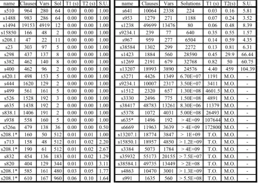
6.1 All-SAT Solver
Figure 6 shows the performance of our new All-SAT solver. The problems are CNF representations of the transition relations of the models in the benchmark. In cases where a model name is followed by ‘*’, the instance consists of multiple transitions and initial conditions of a model. The important variables were arbitrarily chosen.
The table clearly shows a significant speedup for all problems that the blocking clauses method could solve. Smaller number of clauses shortens the time of the bcp() procedure, and also allows more work to be performed in higher levels of the memory hierarchy (main memory and cache). The speedup increases with the hardness of the problem and the computation time.
Our solver is capable of solving larger instances, for which the blocking clauses method runs out of memory. The number of solutions for these instances is simply
name Clauses Vars Sol T1 (s) T2 (s) S.U. name Clauses Vars Solutions T1 (s) T2(s) S.U. s510 964 280 64 0.00 0.00 1.00 s641 10064 2338 224 0.03 0.16 5.81 s1488 983 286 64 0.00 0.00 1.00 s953 1279 271 1188 0.07 0.24 3.52 s1494 19153 4919 12 0.00 0.00 1.00 s1238 49699 13476 80 0.06 0.48 8.39 s15850 166 48 2 0.00 0.00 1.00 s9234.1 239 77 640 0.35 0.55 1.57 s208.1 47 22 11 0.00 0.00 1.00 s967 959 277 6504 0.14 0.59 4.35 s23 303 97 5 0.00 0.00 1.00 s38584 1302 299 2272 0.13 0.81 6.31 s298 437 137 8 0.00 0.00 1.00 s1423 1884 560 28590 0.45 29.9 66.44 s382 462 140 8 0.00 0.00 1.00 s1269 2191 679 32768 0.82 50 60.75 s400 462 96 2 0.00 0.00 1.00 s13207 18993 3890 24576 4.40 459 104.39 s420.1 498 153 5 0.00 0.00 1.00 s3271 4426 1349 6.70E+07 1191 M.O. -s444 1620 129 2 0.00 0.00 1.00 s9234.1 10007 2317 3.50E+07 3411 M.O. -s499 561 161 5 0.00 0.00 1.00 s1512 2320 657 1.30E+08 4601.5 M.O. -s526 1528 192 3 0.00 0.00 1.00 s3330 2496 775 1.50E+08 4891 M.O. -s635 1438 192 2 0.00 0.00 1.00 s38417 48783 13261 8.30E+06 11379 M.O. -s838.1 1406 191 2 0.00 0.00 1.00 s5378 1072 4031 5.00E+08 26493 M.O. -s938 558 160 5 0.00 0.00 1.00 s635* 1496 192 > 4E+09 107644 M.O. -s526n 479 138 36 0.00 0.00 0.50 s6669 11963 3639 > 4E+09 172800 M.O. -s208.1* 160 50 512 0.01 0.01 1.00 s13207.1 18774 3847 > 1E+09 T.O. M.O. -s713 158 48 512 0.01 0.02 2.20 s15850.1 18957 4850 > 1.2E+09 T.O. M.O. -s208.1* 190 61 512 0.01 0.02 2.67 s3384 5073 1784 > 4E+09 T.O. M.O. -s832 454 136 183 0.01 0.02 1.29 s35932 55173 20155 > 7.5E+07 T.O. M.O. -s820 404 129 344 0.01 0.03 3.11 s38584.1 49735 13449 > 2E+08 T.O. M.O. -s208.1* 585 161 480 0.03 0.05 1.77 s4863 10470 3001 > 1.3E+09 T.O. M.O. -s208.1* 610 167 960 0.06 0.10 1.64 s991 1635 560 > 5.5E+08 T.O. M.O.
-Fig. 6. All-SAT solving time. Vars: The number of variables in the problem. About half the
vari-ables are important. Sol: The number of solutions found. T1: The time required for our new All-SAT solver, T2: The time required for the blocking clauses-based algorithm. M.O.: Memory Out. S.U.: Speedup - the ratio T2/T1. The timeout was set to 48 hours.
too high to store in main memory as clauses. In contrast, using our new method, the solutions can be stored on the disk or in the memory of neighboring machines.
The last seven rows in the table show instances for which our solver timed out. In none of these cases, despite the huge number of solutions found (much larger than the size of the main memory in the machine employed), did the solver run out of memory. 6.2 Reachability
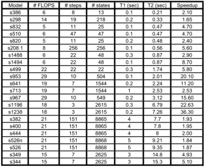
Figure 7 shows the performance of our reachability analysis tool, calculating reacha-bility for the benchmark models. Since [6] and [18] are the only reachareacha-bility analysis algorithms that, as far as we know, depend solely on SAT procedures, the table shows a comparison with the performance reported in [6]. Figure 8 shows the instances for which the reachability analysis did not complete. Here, again, a comparison to [6] is shown. The tables show significant speedup for the completed problems, and deeper steps for those not completed.
7
Conclusions
In this work we presented an All-SAT engine which efficiently finds all the assignments to a subset of the variables, which can be extended to solutions to a given propositional
Model # FLOPS # steps # states T1 (sec) T2 (sec) Speedup s386 6 8 13 0.1 0.21 2.10 s298 14 19 218 0.2 0.33 1.65 s832 5 11 25 0.1 0.47 4.70 s510 6 47 47 0.1 0.47 4.70 s820 5 11 25 0.2 0.48 2.40 s208.1 8 256 256 0.1 0.56 5.60 s1488 6 22 48 0.3 0.87 2.90 s1494 6 22 48 0.1 0.87 8.70 s499 22 22 22 0.3 1.74 5.80 s953 29 10 504 0.1 2.01 20.10 s641 19 7 1544 0.2 2.24 11.20 s713 19 7 1544 1 2.53 2.53 s967 29 10 549 0.2 3.12 15.60 s1196 18 3 2615 0.3 6.79 22.63 s1238 18 3 2615 0.2 7.26 36.30 s382 21 151 8865 4 7.7 1.93 s400 21 151 8865 4 7.8 1.95 s444 21 151 8865 4 8 2.00 s526n 21 151 8868 5 9.21 1.84 s526 21 151 8868 5 9.35 1.87 s349 15 7 2625 3 14.8 4.93 s344 15 7 2625 3 15.3 5.10
Fig. 7. Reachability Analysis Performance. #FLOPS is the number of flip-flops in the model.
#states is the total number of reachable states. T1 is the time required for our tool. T2 is the time as given in [6] using 1.5Ghz dual AMD Athlon cpu with 3GB RAM.
Actual time for max depth (sec) Max depth Completed Time to reach Depth 1 (sec) Depth 1 (1000 sec') #FLOPS Model 10 1 10 1 37 S1269 615 4 28 3 74 S1423 140 3 8 2 669 S13207 31761 23 70 4 57 S1512 251764 111 314 8 228 S9234 8467 7 192 5 597 S15850 2134 4 1 2 1452 S38584
Fig. 8. Reachability Analysis Performance. ‘Depth 1’ is the maximal depth reached in [6] with
timeout of 1000 seconds. ‘Time to reach Depth 1’ is the time required for our tool to complete the same depth. The ‘Max depth’ and the ‘Actual time for max depth’ are the maximal steps successfully completed by our tool, and the time required for it. The Timeout is generally 3600 seconds (1 hour), with longer timeouts for s1512, s9234 and s15850.
formula. We achieve this goal by incorporating a backtrack search and a conflict driven search into one complete engine. Our engine’s memory requirements are independent of the number of solutions. This implies that, during the computation, the number of solutions already found does not become a parameter of complexity in finding further solutions. It also implies that the size of the instance being solved fits in smaller and faster levels of the memory hierarchy. As a result, our method is faster than blocking clause-based methods, and can solve instances that produce solution sets too large to fit
in memory. We have demonstrated how to use our All-SAT engine for memory-efficient reachability computation.
References
1. I. Beer, S. Ben-David, and A. Landver. On-the-fly model checking of RCTL formulas. In
10th Computer Aided Verification, pages 184–194, 1998.
2. A. Biere, A. Cimatti, E. M. Clarke, M. Fujita, and Y. Zhu. Symbolic model checking using SAT procedures instead of BDDs. In DAC. IEEE Computer Society Press, June 1999. 3. Elazar Birnbaum and Eliezer L. Lozinskii. The good old davis-putnam procedure helps
counting models. Journal of Artificial Intelligence Research, 10:457–477, 1999.
4. R. E. Bryant. Graph-based algorithms for boolean function manipulation. IEEE transactions
on Computers, C-35(8):677–691, 1986.
5. J. R. Burch, E. M. Clarke, K. L. McMillan, D. L. Dill, and L. J. Hwang. Symbolic model checking:1020states and beyond. Information and Computation, 98(2):142–170, June 1992. 6. P. Chauhan, E. M. Clarke, and D. Kroening. Using SAT based image computation for
reach-ability analysis. Technical Report CMU-CS-03-151, Carnegie Mellon University, 2003. 7. P. P. Chauhan, E. M. Clarke, and D. Kroening. A SAT-based algorithm for reparameterization
in symbolic simulation. In DAC, 2004.
8. M. Davis, G. Logemann, and D. Loveland. A machine program for theorem proving. CACM, 5(7), July 1962.
9. M. Davis and H. Putnam. A computing procedure for quantification theory. JACM, 7(3):201– 215, July 1960.
10. E. Goldberg and Y. Novikov. Berkmin: A fast and robust SAT-solver. In DATE, 2002. 11. Aarti Gupta, Zijiang Yang, Pranav Ashar, and Anubhav Gupta. SAT-based image
computa-tion with applicacomputa-tion in reachability analysis. In FMCAD, LNCS 1954, 2000.
12. Roberto J. Bayardo Jr. and Joseph Daniel Pehoushek. Counting models using connected components. In AAAI/IAAI, pages 157–162, 2000.
13. H. J. Kang and I. C. Park. SAT-based unbounded symbolic model checking. In DAC, 2003. 14. S. K. Lahiri, R. E. Bryant, and B. Cook. A symbolic approach to predicate abstraction. In
CAV. LLNCS 2725, July 2003.
15. R. Letz. Advances in decision procedures for quantified boolean formulas. In IJCAR, 2001. 16. Chu Min Li and Anbulagan. Heuristics based on unit propagation for satisfiability problems.
In IJCAI (1), pages 366–371, 1997.
17. J.P. Marques-Silva and K.A. Sakallah. Conflict analysis in search algorithms for proposi-tional satisfiability. In IEEE ICTAI, 1996.
18. Ken L. McMillan. Applying SAT methods in unbounded symbolic model checking. In
Com-puter Aided Verification, 2002.
19. M.W. Moskewicz, C.F. Madigan, Y. Zhao, L. Zhang, and S. Malik. Chaff: engineering an efficient SAT solver. In 39th Design Aotomation Conference (DAC’01), 2001.
20. D. Plaisted. Method for design verification of hardware and non-hardware systems. United States Patents, 6,131, 078, October 2000.
21. D. Roth. On the hardness of approximate reasoning. Artificial Intelligence, 82(1-2), 1996. 22. S. Sapra, M. Theobald, and E. M. Clarke. SAT-based algorithms for logic minimization. In
ICCD, 2003.
23. Ofer Shtrichman. Tuning SAT checkers for bounded model checking. In CAV, 2000. 24. Berkeley University of California. Espresso, two level boolean minimizer, 1990.
25. A. Yadgar. Solving All-SAT problem for reachability analysis. M.Sc. thesis, Technion, Israel Institute of Technology, Department of Computer Schience, 2004.
26. H. Zhang. SATO: An efficient propositional prover. In (CADE), 1997.
27. L. Zhang, C. F. Madigan, M. W. Moskewicz, and S. Malik. Efficient conflict driven learning in boolean satisfiability solver. In ICCAD, 2001.