Memory Efficient All-Solutions SAT Solver
and its Application for Reachability Analysis
Orna Grumberg
Assaf Schuster
Avi Yadgar
Computer Science Department, Technion, Haifa, Israel
Abstract
This work presents a memory-efficient All-SAT engine which, given a proposi-tional formula over sets of important and non-important variables, returns the set of all the assignments to the important variables, which can be extended to solu-tions (satisfying assignments) to the formula. The engine is built using elements of modern SAT solvers, including a scheme for learning conflict clauses and non-chronological backtracking. Re-discovering solutions that were already found is avoided by the search algorithm itself, rather than by adding blocking clauses. As a result, the space requirements of a solved instance do not increase when solutions are found. Finding the next solution is as efficient as finding the first one, making it possible to solve instances for which the number of solutions is larger than the size of the main memory.
We show how to exploit our All-SAT engine for performing image computation and use it as a basic block in achieving full reachability which is purely SAT-based (no BDDs involved).
We implemented our All-SAT solver and reachability algorithm using the state-of-the-art SAT solver Chaff [23] as a code base. The results show that our new scheme significantly outperforms All-SAT algorithms that use blocking clauses, as measured by the execution time, the memory requirement, and the number of steps performed by the reachability analysis.
1
Introduction
This work presents a memory-efficient All-SAT engine which, given a propositional formula over sets of important and non-important variables, returns the set of all the assignments to the important variables, which can be extended to solutions (satisfying assignments) to the formula. The All-SAT problem has numerous applications in AI [25] and logic minimization [26]. Moreover, many applications require the ability to instantiate all the solutions of a formula, which differ in the assignment to only a subset of the variables. In [17] such a procedure is used for predicate abstraction. In [8] it is used for re-parameterization in symbolic simulation. In [22, 7] it is used for reachability analysis, and in [16] it is used for pre-image computation. Also, solving QBF is actually solving such a problem, as shown in [18].
Most modern SAT solvers implement the DPLL[10, 9] backtrack search. These solvers add clauses to the formula in order to block searching in subspaces that are known to contain no solution. All-SAT engines that are built on top of modern SAT solvers tend to extend this method by using additional clauses, called blocking clauses,
to block solutions that were already found [22, 7, 16, 17, 8, 24]. However, while the addition of blocking clauses prevents repetitions in solution creation, it also signifi-cantly inflates the size of the solved formula. Thus, the engine slows down in accord with the number of solutions that were already found. Eventually, if too many solutions exist, the engine may saturate the available memory and come to a stop.
In this work we propose an efficient All-SAT engine which does not use block-ing clauses. Given a propositional formula and sets of important and non-important variables, our engine returns the set of all the assignments to the important variables, which can be extended to solutions to the formula. Setting the non-important vari-ables set to be empty yields all the solutions to the formula. Similar to previous works, our All-SAT solver is also built on top of a SAT solver. However, in order to block known solutions, it manipulates the backtracking scheme and the representation of the implication graph. As a result, the size of the solved formula does not increase when solutions are found. Moreover, since found solutions are not needed in the solver, they can be stored in external memory (disk or the memory of another computer), pro-cessed and even deleted. This saving in memory is a great advantage and enables us to handle very large instances with huge number of solutions. The memory reduction also implies time speedup, since the solver handles much less clauses. In spite of the changes we impose on backtracking and the implication graph, we manage to apply many of the operations that made modern SAT solvers so efficient. We derive conflict clauses based on conflict analysis, apply non-chronological backtracking to skip sub-spaces which contain no solutions, and apply conflict driven backtracking under some restrictions.
We show how to exploit our All-SAT engine for reachability analysis, which is an important component of model checking. Reachability analysis is often used as a preprocessing step before checking. Moreover, model checking of most safety tempo-ral properties can be reduced to reachability analysis [1]. BDD-based algorithms for reachability are efficient when the BDDs representing the transition relation and the set of model states can be stored in memory [5, 6]. However, BDDs are quite unpredictable and tend to explode on intermediate results of image computation. When using BDDs, a great effort is invested in improving the variables order, which strongly influences the BDD’s size. SAT-based algorithms, on the other hand, can handle models with larger number of variables. However, they are mainly used for Bounded Model Checking (BMC) [2].
Pure SAT-based methods for reachability [22, 7] and model checking of safety properties [16, 24] are based on All-SAT engines, which return the set of all the solu-tions to a given formula. The All-SAT engine receives as input a propositional formula describing the application of a transition relationT to a set of statesS. The resulting
set of solutions represents the image of S (the set of all successors for states inS).
Repeating this step, starting from the initial states, results in the set of all reachable states.
Similar to [22, 7], we exploit our All-SAT procedure for computing an image for a set of states, and then use it iteratively for obtaining full reachability. Several optimiza-tions are applied at that stage. Their goals are to reduce the number of found soluoptimiza-tions by avoiding repetitions between images; to hold the found solutions compactly; and to keep the solved formula small.
An important observation is that for image computation, the solved formula is de-fined over variables describing current statesx, inputsI, next statesx
0, and some
aux-iliary variables that are added while transforming the formula to CNF. However, many solutions to the formula are not needed: the only useful ones are those which give
different values tox 0
. This set of solutions is efficiently instantiated by our algorithm by definingx
0
as the important variables. Since the variables inx 0
typically constitute just 10% of all the variables in the formula [28], the number of solutions we search for, produce, and store, is reduced dramatically. This was also done in [22, 7, 16, 24]. Note, that by definingxas the important variables, our engine can perform pre-image
computation, and thus can be used whenever such a procedure is required. However, in our experiments, it was only employed for image computation.
We have built an All-SAT solver based on the state-of-the-art SAT solver Chaff [23]. Experimental results show that our All-SAT algorithm outperforms All-SAT algorithms based on blocking clauses. Even when discovering a huge number of solutions, our solver does not run out of memory, and does not slow down. Similarly, our All-SAT reachability algorithm also achieves significant speedups over blocking clauses-based All-SAT reachability, and succeeds to perform more image steps.
The rest of the paper is organized as follows. Section 2 presents related work. Section 3 gives the background needed for this work. Sections 4 and 5 describe our algorithm and its implementation. A proof for the algorithm’s correctness is given in Section 6. Section 7 describes the utilization of our algorithm for reachability analysis. Section 8 shows our experimental results, and Section 9 includes conclusions.
2
Related Work
In [7] an optimization is employed to the blocking clauses method. The number of blocking clauses and the run time are reduced significantly by inferring from a newly found solution a set of related solutions, and blocking them all with a single clause. This, however, is insufficient when larger instances are considered. Moreover, the opti-mization is applicable only for formulae which originated from a model, and therefore, is not applicable for solving other QBF as described in the introduction.
In [19, 27] a success-driven learning is used. This method uses a hash table to store information about solutions found in sub-spaces which were already searched. While this information helps reducing the search time, it still implies growth of the solved instance. Moreover, this method depends on the fact that the CNF originates from a model, and is used for pre-image computation only, where the values of the ’next-state’ variables are used as objectives for the SAT procedure to satisfy.
In [4, 15] all the solutions of a given propositional formula are found by repeat-edly choosing a value to one variable, and splitting the formula accordingly, until all the clauses are satisfied. However, in this method, all the solutions of the formula are found, and distinguishing between important and non-important variables is not straight forward. This method can not be efficiently applied for quantifier elimination and image computation, since finding all the solutions for the formulae implies repeti-tive instantiation of the same ’next state’.
Other works also applied optimizations within a single image [7] and between im-ages [22, 7]. These have similar strength to the optimization we apply between imim-ages. However, within an image computation we gain significant reductions in memory and time due to our new All-SAT procedure, and the ability to process the solutions outside the engine before the completion of the search. This gain is extended to the reachability computation as well, as demonstrated by our experimental results.
In [14], a hybrid method of SAT and BDD is proposed for image computation. This implementation of an All-SAT solver does not use blocking clauses. The known solutions are kept in a BDD which is used to restrict the search space of the All-SAT engine. While this representation might be more compact than blocking clauses, the
All-SAT engine still depends on the set of known solutions when searching for new ones. We believe that our algorithm can be used to enhance the performance of such hybrid methods as well.
3
Background
3.1
The SAT Problem
Let an assignmentAto a set of Boolean variablesvbe a functionA:v!ftrue;falseg.
Given a Boolean formula'(v), the Boolean Satisfiability Problem (SAT) is the
prob-lem of finding an assignmentA tov such that'(v)will have the value ‘true’ under
this assignment. Such an assignment is called a satisfying assignment, or a solution, for'. A partial assignmentA
0
is a partial function, for which the domain isv 0 v. If v 0 2(vnv 0 )thenA 0 (v 0
)is undefined. The SAT problem is an NP-Complete problem,
thus believed to have exponential worst case complexity [12].
We shall discuss formulae presented in the conjunctive normal form (CNF). That is,'is a conjunction of clauses, while each clause is a disjunction of literals overv. A
literallis an instance of a variable or its negation:l2fv;:vjv2vg. We define the
value of a literallunder an assignmentAto be A(l) =
A(v) l=v
:A(v) l=:v
. We shall consider a clause as a set of literals, and a formula as a set of clauses.
A clauselis satisfied under an assignmentAif and only if9l2l;A(l)=true.
We denote this by A l. For a formula ' given in CNF, and an assignmentA, A',8l2';Al. Hence, if, under an assignment (or a partial assignment)A,
all of the literals of some clause in'are false, thenAdoes not satisfy'. Formally:
9l2'suhthat8l2l;A(l)=false
)A2' (1)
We such a situation a conflict, and say thatAconflicts with'. We can therefore
look at the clauses of the formula as constraints which the assignments should satisfy. Each clause is a constraint, and satisfying all the clauses means satisfying the formula. For a formula'given in CNF, we can apply resolution on its clauses. For each
two clauses 1
;
2, if a variable
vexists, such that 1
=A[fvgand 2
=B[f:vg,
whereA andB are sets of literals, then resolution( 1 ; 2 ) = A[B. For r = resolution( 1 ; 2 );') r, and ''^
r[10]. That is, by using resolution we can
add new clauses to', and the new formula will be equivalent to'.
3.2
Davis-Putnam-Logemann-Loveland Backtrack Search (DPLL)
We begin by describing the Boolean Constraint Propagation (bcp()) procedure. Given a partial assignmentAand a clausel, if there is one literall 2 lsuch thatA(l)is
undefined, while the rest of the literals are all false, then in order to avoid a conflict,
Amust be extended such thatA(l)=true. lis called a unit clause or an asserting clause, and the assignment to lis called an implication. An asserting clause which
implies the literallis its antecedent, referred to as ante(l). An example for an asserting
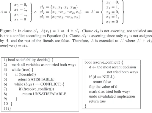
clause is given in Figure 1. Once the assignment is extended, other clauses may become asserting, and the assignment has to be extended again. The bcp() procedure finds all the possible implications in a given moment (iteratively) and returns CONFLICT if a conflict as described in Equation (1) occurs, and NO CONFLICT otherwise. This procedure is efficiently implemented in [23, 13, 30, 21, 20].
A= 8 > > < > > : x 0 =0; x1=1; x 3 =1; x5=0 9 > > = > > ; ^ l1=fx0;x1;x2;x10g l 2 =fx 0 ;:x 1 ;:x 2 ;x 4 g l 3 =fx 0 :x 2 ;:x 3 ;x 5 g )A 0 = > > > > < > > > > : x 0 =0; x1=1; x 2 =0 ; x 3 =1; x5=0 > > > > = > > > > ;
Figure 1: In clausel1,A(x1)=1)A l1. Clausel2is not asserting, not satisfied and
is not a conflict according to Equation (1). Clausel3is asserting since onlyx2is not assigned
byA, and the rest of the literals are false. Therefore, Ais extended toA 0 whereA 0 l 3. ante(:x2)=l3.
1) bool satisfiability decide()f
2) mark all variables as not tried both ways 3) while (true)f 4) if (!decide()) 5) return SATISFIABLE; 6) while (bcp() == CONFLICT)f 7) if (!resolve conflict()) 8) return UNSATISFAIABLE 9) g 10 g 11)g (a) DPLL
bool resolve conflict()f
d the most recent decision not tried both ways if (d == NULL)
return false flip the value of d mark d as tried both ways undo invalidated implication return true
g
(b) Resolve Conflict
Figure 2:DPLL Backtrack Search. The procedure decide() chooses one of the free variables and assigns a value to it. If no such variable exists, it returns ‘false’. The procedure resolve conflict() performs chronological backtracking.
The DPLL algorithm [10, 9] walks the binary tree which describes the variables space. At each step, a decision is made. That is, a value to one of the variables is chosen, thus reaching deeper in the tree. Each decision is assigned with a new decision
level. After a decision is made, the algorithm uses the bcp() procedure to compute
all its implications. All the implications are assigned with the corresponding decision level. If a conflict is reached, the algorithm backtracks in the tree, and chooses a new value to the most recent variable for which a decision was made, such that the variable was not yet tried both ways. This is called chronological backtracking. The algorithm terminates if one of the leaves is reached with no conflict, describing a satisfying as-signment, or if the whole tree was searched and no satisfying assignment was found, meaningis unsatisfiable. The pseudo code of this algorithm is shown in Figure 2.
3.3
Optimizations
Current state of the art solvers use Conflict Analysis, Learning and Conflict Driven backtracking to optimize the DPLL algorithm as described below;
3.3.1 Implication Graphs
An Implication Graph represents the current partial assignment during the solving pro-cess, and the reason for the assignment to each variable. For a given assignment, the implication graph is not unique, and depends on the decisions and the order used by the
bcp(). Recall that we denote the asserting clause that implied the value oflbyante(l),
partial assignmentA:
The implication graph is a directed acyclic graphG(L;E).
The vertices are the literals of the current partial assignment:8l2L;l2fv;:vj v2V ^A(l)=trueg.
The edges are the reasons for the assignments: E = (l i ;l j ) j l i ;l j 2 L;l i 2 ante(l j
) . That is, for each vertex l, the incident edges represent the clause ante(l). A decision vertex has no incident edge.
Each vertex is also assigned with the decision level of the corresponding variable.
In an implication graph with no conflicts, there is at most one vertex for a variable. When a conflict occurs, there are both true and false vertices of some variable, denoted
conflicting variable. In case of a conflict, we only consider the connected component
of the graph which includes the conflict vertices, since the rest of the graph is irrelevant to the analysis.
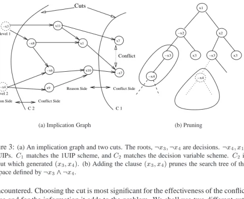
A Unique Implication Point (UIP) in an implication graph is a vertex of the current decision level, through which all the paths from the decision vertex of this level to the conflict pass. There may be more than one UIP, and we order them starting from the conflict. The decision variable of a level is always a UIP, since it is the first vertex of all the paths in the corresponding level.
An implication graph with a conflict and 2 UIPs is presented in Figure 3(a). 3.3.2 Conflict Analysis and Learning
Upon an occurrence of a conflict, we perform conflict analysis, which finds the reason to it and adds constraints over the search space accordingly. The conflict analysis is performed over the implication graph as described next :
The graph is bi-partitioned such that all the decision variables are on one side
(the reason side) and the conflicting variable is on the other side (the conflict side). We call this bi-partitioning a cut. The reason for the conflict is defined by all the vertices on the reason side with at least one edge to the conflict side. These vertices are the reason literals.
In order for the conflict not to re-occur, the current assignment to the reason
vari-ables should not occur. Therefore, a new clause is generated, which is comprised of the negation of the reason literals. This clause is called a conflict clause.
The conflict clause is added to the problem’s formula.
The conflict clauses added to the problem can be viewed as constraints over the search space, thus pruning the search tree by preventing the solver from reaching the subspace of the reason for the last conflict again. Note that the conclusion of the learn-ing, which is expressed by the conflict clause, is correct regardless of the assignment to the variables. The generation of the new clause is actually applying resolution on the original clauses. Therefore, the new problem is equivalent to the original.
Figure 3(a,b) shows an implication graph which is used to generate a conflict clause, and the way it prunes the search tree.
Different cuts, corresponding to different learning schemes, will result in different conflict clauses. Moreover, more than one clause can be added when a single conflict
Cuts
C 1 C 2
Reason Side Conflict Side
Conflict
Reason Side Conflict Side level 1 level 2 x11 −x6 −x7 −x3 x1 x7 −x8 x9 x10 −x4
(a) Implication Graph
−x3 x3 x1 −x3 −x2 x2 −x4 x3 −x4 (b) Pruning
Figure 3:(a) An implication graph and two cuts. The roots,:x 3 ;:x 4are decisions. :x 4 ;x 10
are UIPs. C1matches the 1UIP scheme, andC2matches the decision variable scheme. C2 is
the cut which generated(x 3
;x 4
). (b) Adding the clause(x 3
;x 4
)prunes the search tree of the
subspace defined by:x 3
^:x 4.
is encountered. Choosing the cut is most significant for the effectiveness of the conflict clause and for the information it adds to the problem. We shall use two different cuts in our work that will generate clauses involving:
1. The first UIP (1UIP); i.e., The one which is closest to the conflict. 2. The decision variable of the current level, which is also a UIP.
We want a cut that will generate a conflict clause with only one variable from the highest decision level. Such a cut is achieved when a UIP is placed on the reason side, and all the vertices assigned after it are placed on the conflict side. The UIP (the negation of the literal in the graph) would then be the only variable from the highest decision level in the conflict clause. Figure 3(a) shows the cuts corresponding to the suggested schemes. This kind of a conflict clause is effective as we explain next.
Letbe the generated conflict clause andmthe current decision level. In order to
resolve the conflict, we backtrack one level and invalidate all of its assignments. The UIP was the only literal in from levelm, thus, it is the only variable inwith no
value. Recall that the literals inare the negation of the current values to the reason
variables, making them all false under the current assignment. The result is that the conflict clause is now a unit clause, and therefore is asserting. The unit literal in the conflict clause is the negation of the UIP. Thus, flipping the value of the UIP variable (not necessarily the decision) is now an implication of the assignments in the lower levels and the added conflict clause.
3.3.3 Conflict Driven Backtracking
In order to emphasize the recently gained knowledge, conflict driven backtracking is used: Letlbe the highest level of an assigned variable in the conflict clause. The solver
discards some of its work by invalidating all the assignments abovel. The implication
in the search tree. The result of this backtrack is ‘jumping’ into a new search space, as shown in Figure 4. Note that the other variables for which the assignments were invalidated, may still assume their original values, and lead to a solution.
1 0 0 0 0 0
Conflict
x3 x2 x1 x4 x1 x4Figure 4: Conflict driven backtracking after adding the conflict clause(x 1
;x 4
)creates a new
variables order.x
3is now free to assume either true or false value.
3.4
The All-SAT Problem
Given a Boolean formula presented in CNF, the All-SAT problem is to find all of its solutions as defined by the SAT problem.
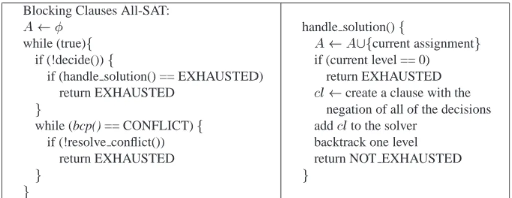
The Blocking Clauses Method
A straightforward method to find all of the formula’s solutions is to modify the DPLL SAT solving algorithm such that when a solution is found, a blocking clause describing its negation is added to the solver. This clause prevents the solver from reaching the same solution again. The last decision is then reversed, and the search is continued normally. At any given time, the solver holds a formula representing the original formula and the negation of all of the solutions found so far. Once all the solutions are found, there is no satisfying assignment to the current formula, and the algorithm terminates.
This algorithm suffers from rapid space growth as it adds a clause of the size ofv
for each solution found. Another problem is that the increasing number of clauses in the system will slow down the bcp() procedure which will have to look for implications in an increasing number of clauses.
An improvement for this algorithm can be achieved by generating a clause consist-ing of the negation of the decision literals only, since all the rest of the assignments are implications and are forced by these decisions. This reduces the size of the generated clauses dramatically (1-2 orders of magnitude) but does not affect their number.
The blocking clauses algorithm with the described optimization is shown in Figure 5. Variations of this algorithm were used in [22, 7, 16], where the All-SAT problem is solved for model checking. In the next section, we present a new All-SAT algorithm which is fundamentally different from the blocking clauses method.
Blocking Clauses All-SAT:
A
while (true)f
if (!decide())f
if (handle solution() == EXHAUSTED) return EXHAUSTED g while (bcp() == CONFLICT)f if (!resolve conflict()) return EXHAUSTED g g handle solution()f
A A[fcurrent assignmentg
if (current level == 0) return EXHAUSTED
l create a clause with the
negation of all of the decisions addlto the solver
backtrack one level return NOT EXHAUSTED
g
Figure 5: All SAT algorithm using blocking clauses to prevent multiple instantiations of the same solution. The procedures bcp() , decide() and resolve conflict() are the same as those defined for DPLL in section 2. At the end of the process,Ais the set of all the solutions to the
problem.
4
Memory efficient All-SAT Algorithm
4.1
Conventions
Assume we are given a partition of the variables to important and non-important vari-ables. Two solutions to the problem which differ in the non-important variables only are considered the same solution. Thus, a solution is defined by a subset of the vari-ables.
A subspace of assignments, defined by a partial assignment, is the set of all
assignments which agree with on its assigned variables. A subspace is called ex-hausted if all of the satisfying assignments in it (if any) were already found. At any
given moment, the current partial assignment defines the subspace which is now being investigated. However, it is enough to consider the decision variables only. This is correct because the rest of the assignments are implied by the decisions.
4.2
The All-SAT Algorithm
Our algorithm walks the search tree of the important variables. We call this tree the
im-portant space. Each leaf of this tree represents an assignment to the imim-portant variables
which does not conflict with the formula. When reaching such a leaf, the algorithm tries to extend the assignment over the non-important variables. Hence, it looks for a solu-tion within the subspace defined by the important variables. Note that the walk over the
important space should be exhaustive, while only one solution for the non-important
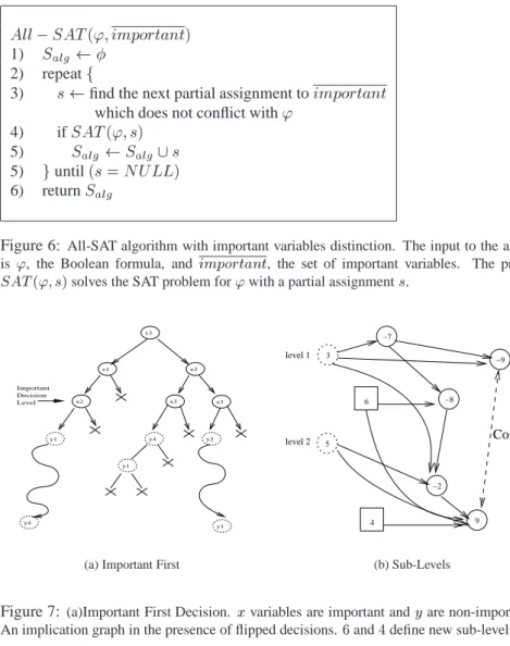
variables should be found. A pseudo code of this algorithm is given in Figure 6, and it is illustrated in Figure 7(a).
We incorporate these two behaviors into one procedure by modifying the decision and backtracking procedures of a conflict driven backtrack search, and the representa-tion of the implicarepresenta-tion graph.
Important First Decision Procedure: We create a new decision procedure which looks for an unassigned variable from within the important variables. If no such vari-able is found, the usual decision procedure is used to choose a varivari-able from the non-important set. The procedure returns ’true’ if an unassigned variable was found, and ’false’ otherwise. This way, at any given time, the decision variables are a sequence of important variables, followed by a sequence of non important variables. At any given
1) S alg
2) repeatf
3) s find the next partial assignment toimportant
which does not conflict with'
4) ifSAT(';s) 5) S alg S alg [s 5) guntil(s=NULL) 6) returnS alg
Figure 6: All-SAT algorithm with important variables distinction. The input to the algorithm is ', the Boolean formula, andimportant, the set of important variables. The procedure SAT(';s)solves the SAT problem for'with a partial assignments.
y1 y2 y4 y1 Important Level Decision x2 x3 x3 x2 x1 x3 y1 y4
(a) Important First
Conflict level 1 6 4 level 2 3 5 −7 9 −2 −8 −9 (b) Sub-Levels
Figure 7: (a)Important First Decision. xvariables are important andyare non-importnat. (b)
An implication graph in the presence of flipped decisions.6and4define new sub-levels.
time, the important decision level is the maximal level in which an important variable is a decision. An example is given in Figure 7(a).
Exhaustive Walk of the Important Space: An exhaustive walk of the important space is performed by extending the original DPLL algorithm with the following procedures: Chronological backtracking after a leaf of the important space, representing an assign-ments to the important variables, is handled; Learning a conflict clause and chrono-logical backtracking upon an occurrence of a conflict; Non-chronochrono-logical backtracking when a subspace of the problem is proved to be exhausted.
Chronological backtracking is performed when the current subspace is exhausted. It means that, under the previous decisions, the last decision variable must assume a new value. Hence, its reverse assignment can be seen as an implication of the previous decisions. We therefore flip the highest decision and assign it with the level below. This way, the highest decision is always the highest decision not yet flipped. Higher decisions which were already flipped are regarded as its implications. Note, though, that there is no clause implying the values of the flipped decisions. Therefore, a new definition for the implication graph is required.
We change the definition of the implication graph as follows: Root vertices in the graph still represent the decisions, but also decisions flipped because of previous chronological backtracking. Thus, for conflict analysis purposes, a flipped decision is considered as defining a new decision sub-level. The result is a graph in which the nodes represent the actual assignments to the variables, and the edges represent clauses. Therefore, this graph is an implication graph, as defined in Section 3.3.1. This graph describes the current assignment, though not the current decisions. An example for such a graph is given in Figure 7(b). Recall that generating a new conflict clause using an implication graph is equivalent to applying resolution on clauses of the formula, represented by the graph’s edges. Such a new clause is derived from the formula, and is independent of the current decisions. Since our newly defined graph corresponds to the definition of an implication graph, we can use it in order to derive a new conflict clause, which can be added to the formula, without changing its set of solutions.
We perform the regular conflict analysis, which leads to a UIP in the newly defined sub-level. The generated conflict clause is added to the formula to prune the search tree, as for solving the SAT problem. Modifying the implication graph and introducing the new sub-levels may cause the conflict clause not to be asserting. However, since we do not use conflict driven backtracking in the important space, our solver does not require that the conflict clauses will be asserting. A non-asserting clause is added to the formula, so that it might prune the search tree in the future, and the search is then resumed.
We now consider the case in which a conflict clause is asserting. In this case, we extend the current assignment according to it. Let
1be a conflict clause, and litits
implication. Addinglitto the current assignment may cause a second conflict, for
whichlitis the reason. Therefore, we are able to perform conflict analysis again, using litas a UIP. The result is a second conflict clause,
2 which implies
:lit. It is
ob-vious now that neither of the assignments tolitwill resolve the current conflict. The
conclusion is that the reason for this situation lies in a lower decision level, and that a larger subspace is exhausted. Identifying the exhausted subspace is done by calcu-lating 3 resolution( 1 ; 2
)[10]. We skip it by backtracking to the decision level
preceding the highest level of a variable in
3. This is the level below the highest
de-cision level of a variable in 1or
2. Note that backtracking to any level higher than
that would not resolve the conflict as both 1and
2would imply
litand:lit
respec-tively. Therefore, by this non-chronological backtracking, we skip a large exhausted subspace.
Assigning Non-Important Variables: After reaching a leaf in the important space, we have to extend the assignment to the non important variables. At this point, all the important variables are assigned with some value. Note, that since we only need one extension, we actually have to solve the SAT problem for the given formula with the current partial assignment. This is done by allowing the normal work of the optimized SAT algorithm, including decisions, conflict clause learning, and conflict driven back-tracking. However, we allow backtracking down to the important decision level but not below it, in order not to interfere with the exhaustive search of the important space. If no solution is found, the current assignment to the important variables can not be extended to a solution for the formula, and should be discarded. On the other hand, if a solution to the formula is found, its projection over the important variables is a valid output. In both cases, we backtrack to the important decision level and continue the exhaustive walk of the important space.
1 2 3 4 5 6 ? ? ? ? ? ? ? ? ? ? y -4 2 19 6 -1 3 13 18 7 -9 17 22 11 16 12 -14 (a) Stack ? ? ? ? ? ? ? ? ? ? y -4 2 19 6 -1 3 13 18 7 -9 -17 (b) Backtrack ? ? ? ? ? ? ? ? ? ? y -4 2 19 6 -1 3 13 -18 (c) Chronological Backtrack
Figure 8:(a) A stack. 4;6;18;17;22and16are the decisions. (b) Backtrack to level3. 17
has NULL antecedent. (c) Chronological backtrack.
5
Implementation
We implemented our All-SAT engine using zChaff [23] as a base code. This SAT solver uses the VSIDS decision heuristic [23], an efficient bcp() procedure, conflict clause learning, and conflict driven backtracking. We modified the decision procedure to match our important-first decision procedure, and added a mechanism for chronolog-ical backtracking. We implemented the exhaustive walk over the important space us-ing chronological backtrackus-ing, and by allowus-ing non-chronological backtrackus-ing when subspaces without solutions are detected. We used the original optimized SAT solving procedures above the important decision level, where it had to solve a SAT problem. Next, we describe the modifications imposed on the solver in the important space.
The original SAT engine represents the current implication graph by means of an
assignment stack, hereafter referred to as stack. The stack consists of levels of
assign-ments. The first assignment in each level is the decision, and the rest of the assignments in the level are its implications. Each implication is in the lowest level where it is im-plied. Thus, an implication is implied by some of the assignments prior to it, out of which at least one is of the same level. For each assigned variable, the stack holds its value and its antecedent, where the antecedent of a decision variable is NULL. An example for a stack is given in Figure 8(a).
In the following discussion, backtrack to levelirefers to the following procedure:
a) Flipping the decision in leveli+1. b) Invalidation of all the assignments in levels i+1and above, by popping them out of the stack. c) Pushing the flipped decision at the
end of leveli, with NULL antecedent. d) Executing bcp() to calculate the implications
of the flipped decision. This is shown in Figure 8(a,b)
We perform chronological backtracking from levelj within the important space
by backtracking to levelj 1. This way, the flipped decisions appear as implications
of prior ones, and the highest decision not yet flipped is always the highest in the
stack. The assignments with NULL antecedents, which represent exhausted subspaces,
remain in the stack until a whole subspace which includes them is exhausted. An example for this procedure is given in Figure 8(b,c).
Our stack now includes decision variables, implications, and flipped decisions, which appear as implications but with no antecedents. Using this stack we can con-struct the implication graph according to the new definition given in section 4.2. Thus we can derive a conflict clause whenever a conflict occurs.
Decisions about exhausted subspaces are made during the process of resolving a conflict, as described next. We define a generated clauses stack, which is used to
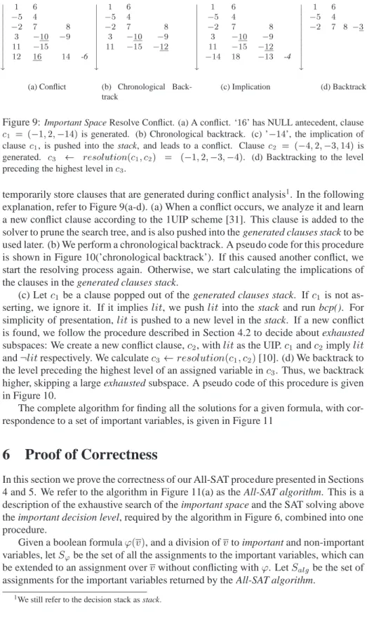
? ? ? ? ? ? ? ? ? ? ? y 1 6 5 4 2 7 8 3 10 9 11 15 12 16 14 -6 (a) Conflict ? ? ? ? ? ? ? ? ? ? ? y 1 6 5 4 2 7 8 3 10 9 11 15 12 (b) Chronological Back-track ? ? ? ? ? ? ? ? ? ? ? y 1 6 5 4 2 7 8 3 10 9 11 15 12 14 18 13 -4 (c) Implication ? ? ? ? ? ? ? ? ? ? ? y 1 6 5 4 2 7 8 3 (d) Backtrack
Figure 9: Important Space Resolve Conflict. (a) A conflict. ‘16’ has NULL antecedent, clause 1 = ( 1;2; 14)is generated. (b) Chronological backtrack. (c) ’ 14’, the implication of
clause
1, is pushed into the stack, and leads to a conflict. Clause
2
= ( 4;2; 3;14)is
generated. 3 resol ution(1;2) = ( 1;2; 3; 4). (d) Backtracking to the level
preceding the highest level in 3.
temporarily store clauses that are generated during conflict analysis1. In the following explanation, refer to Figure 9(a-d). (a) When a conflict occurs, we analyze it and learn a new conflict clause according to the 1UIP scheme [31]. This clause is added to the solver to prune the search tree, and is also pushed into the generated clauses stack to be used later. (b) We perform a chronological backtrack. A pseudo code for this procedure is shown in Figure 10(’chronological backtrack’). If this caused another conflict, we start the resolving process again. Otherwise, we start calculating the implications of the clauses in the generated clauses stack.
(c) Let
1 be a clause popped out of the generated clauses stack. If
1 is not
as-serting, we ignore it. If it implieslit, we pushlitinto the stack and run bcp(). For
simplicity of presentation,litis pushed to a new level in the stack. If a new conflict
is found, we follow the procedure described in Section 4.2 to decide about exhausted subspaces: We create a new conflict clause,
2, with
litas the UIP. 1and
2imply
lit
and:litrespectively. We calculate 3 resolution( 1 ; 2 )[10]. (d) We backtrack to
the level preceding the highest level of an assigned variable in
3. Thus, we backtrack
higher, skipping a large exhausted subspace. A pseudo code of this procedure is given in Figure 10.
The complete algorithm for finding all the solutions for a given formula, with cor-respondence to a set of important variables, is given in Figure 11
6
Proof of Correctness
In this section we prove the correctness of our All-SAT procedure presented in Sections 4 and 5. We refer to the algorithm in Figure 11(a) as the All-SAT algorithm. This is a description of the exhaustive search of the important space and the SAT solving above the important decision level, required by the algorithm in Figure 6, combined into one procedure.
Given a boolean formula'(v), and a division ofvto important and non-important
variables, letS
'be the set of all the assignments to the important variables, which can
be extended to an assignment overvwithout conflicting with'. LetS
algbe the set of
assignments for the important variables returned by the All-SAT algorithm.
Important Space resolve conflict()f
while (conflict_generated clauses.size>0)f
if (conflict)f chronological backtrack 8 > > > < > > > : a) if (current level == 0) b) return FALSE
c) l generate conflict clause with 1UIP, addlto'
d) generated clauses.push(l)
e) backtrack one level
gelsef Implicate Conflict Clauses 8 > > < > > : 1) l1 generated clauses.pop() 2) if (l 1is asserting) f 3) l it unit literal inl 1
4) pushl itinto the stack
Non-Chronological Backtracking 8 > > > > > > > < > > > > > > > : 5) if (bcp() = CONFLICT)f 6) l
2 generate conflict clause with
l itas UIP, add 2to ' 7) l 3 resol utionof(l 1 ;l 2), add 3to ' 8) generatedl auses:push(l 3 )
9) backtrack to the level preceding the highest level inl3
10) g 11)g g g return TRUE g
Figure 10:Important Space resolve conflict.'is the formula being solved.
Theorem 6.1 1)S alg =S ' 2)8s2S
alg, the All-SAT algorithm adds stoS
algexactly once. Proof:
Throughout this proof, we denote the current formula held by the solver at a given moment by'
0
. If the algorithm adds a new clause to the solver, we denote the new formula by'
00
.
The following lemma relates the implication graph defined in our algorithm to the implication graph defined by the SAT solving procedure.
Lemma 6.2 For an implication graph G(V;E), according to the new definition in Section 4.2, there exists an implication graphG
0 (V
0 ;E
0
), according to the definition in Section 3.3.1 whereV
0
=V,E 0
=Eand all the roots ofG 0
are decisions.
Proof: Considerr 1
:::r
k, the roots in graph
Gin the order of their assignment. Each
rootr
iis either a decision or a flipped decision. We consider each such root as defining
a sub-level, as illustrated in Figure 7(b). We have to prove that there existsG
0 (E 0 ;V 0 )whereV 0 =V andE 0 =E, and all the roots inG 0
are decisions. In order to prove this, we have to show an implication graphG
0
wherer 1
:::r
k are roots, and with the same implications and in the same
order in levels1:::k, as the implications in sub-levels1:::kof graphG. We prove
this by induction onr i.
Base case. Fori=1, we have to show that there is an implication graph wherer 1is
the root of level1, and has the same implications in the same order as in sub-level1of
graphG. Considera 1
:::a
n, all the implications in the sub-level
1ofG. This is the set
of all the implications ofr
1. Hence, there is some SAT solving computation
, in which r
1is the first decision, and the bcp() procedure assigns a
1 :::a
1) S alg
2) while (true)f
3) if (!Important-First-decide())f
4) if (handle solution() == EXHAUSTED) 5) returnS
alg
6) g
7) while (bcp() == CONFLICT)f
8) if (current decision level>important decision level)
9) resol ved SAT resolve conflict()
10) else
11) resol ved Important Space resolve conflict()
12) if (!resol ved)
13) returnS alg
12) g
13) g
(a) All-SAT Algorithm
handle solution() 1)S alg S alg [fcurrent assignment to 2) important g
3) if (important decision level == 0) 4) return EXHAUSTED
5) backtrack to important decision level 1
6) return NOT EXHAUSTED
SAT resolve-conflict()
1) l learn a new conflict clause using 1UIP
2) addlto the solver
3) l highest level of a literal inl
4) if(l<important decision level)f
5) if (important decision level == 0) 6) return ‘false’
7) backtrack to important decision level 8) gelsef 9) if (l==0) 10) return ‘false’ 11) backtrack to levell 12) g 13) return ‘true’
(b) Handle Solution (c) SAT Resolve conflict
Figure 11: (a) All-SAT procedure. 'is the Boolean formula, andimportantis the set of
important variables. The procedure Important-First decide() is described in Section 4.2, and the procedure Important Space resolve conflict() is described in Figure 10. (b) The procedure handle solution(). (c) SAT resolve conflict(). This is the regular resolve conflict() procedure, shown in Figure 2(b), limited to backtrack no lower than the important decision level.
The bcp() procedure assigns all the possible implications at a given time. Therefore,
a 1
:::a
nare the only implications assigned by
in level1.
The implication graph corresponding tohasr
1as a root, and a
1 :::a
nas
impli-cations in the order they appear inG, and thus meets our requirements.
Induction step. Given that fori = m < kthere is an implication graph where the
roots arer 1
:::r
m, and the implications in levels
1:::mare the same, and in the same
order, as in sub-levels1::mof graphG, we have to show that there is an implication
graph where the roots arer 1
:::r
m+1, and the implications in levels
1:::(m+1)are
the same, and in the same order, as in sub-levels1::(m+1)of graphG
Since we have a graph where the roots arer 1
:::r
1:::mare the same, and in the same order, as in sub-levels1::mof graphG, we know
that there is a SAT solving computation in which these decisions were made, and those implications were calculated in this specific order. We also know that there were no other implications which do not appear in the implication graph. Note that ifr
m+1is
a decision inG, then it is not implied by its preceding assignments. Also, ifr m+1is a
flipped decision inG, it means that at some earlier point it was a decision with the same
preceding assignments, and therefore is also not implied by them. The conclusion is that there is a SAT solving computation, in which the decisions and implications are
identical to those in sub-levels1:::mof graphG, and in whichr
m+1is not assigned.
This computation can be extended by the decisionr m+1.
Considera 1
:::a
n, the implications in level
m+1in graphG. This is the set of
im-plications of the assignments to the variables in sub-levels1:::m, and tor
m+1in the
graph. We know that these variables are given the same assignments by the computa-tions. Therefore,a
1 :::a
nis the set of implications in level
m+1of the computation . There is, then, an extension toin which the bcp() procedure assignsa
1 :::a
n in
this specific order. The bcp() procedure assigns all the possible implications at a given time. Thus,assigns all the implications ofr
m+1and its preceding assignments, and
them only, and thereforea 1
:::a
n are the only implications calculated by
in level m+1.
The implication graph corresponding tohasr 1
:::r
m+1as roots, the same
impli-cations and in the same order in levels1:::mas in sub-levels1:::mof graphG, and a
1 :::a
nas implications in level
m+1in the order they appear inG, and thus meets
our requirements.
2 Lemma 6.3 When running the All-SAT algorithm, at any given time,'
0 '. Proof: We prove Lemma 6.3 by induction.
Base case. At the beginning of the process,' 0
=' ) '
0 '. Induction step. Assume the current formula'
0
', and a new clausel is going
to be added to the solver such that' 00
= '
0
^l. Consider the All-SAT algorithm. l was generated by one of the resolve conflict() procedures, when executing line9
or11of the algorithm. Therefore, the clause was either created by the procedure
de-scribed in Figure 10 (corresponding to line 11), or by the procedure in Figure 11(c)
(corresponding to line9). We distinguish between the following cases:
1. l was generated in line 7of the algorithm in Figure 10. In this case, l = resolution( 1 ; 2 ), where 1 and 2are clauses in ' 0
. Due to the nature of the
resolution procedure,' 0 ^l' 0 . Therefore,' 00 ' 0 '.
2. lwas generated in line c or6of the algorithm in Figure 10, or in line1of the
algorithm in Figure 11(c). In this case,lwas generated using our newly
de-fined implication graph. According to Lemma 6.2, for each implication graph corresponding to our new definition, we can construct an implication graph with the same vertices and edges, which corresponds to the original definition used by the SAT solving procedure, given in Section 3.3.1. We know that conflict clauses generated from the original implication graphs can be added to the formula with-out changing its set of solutions [31]. Thus, we can use the newly defined graph to generate conflict clauses, and add them to the formula without changing its solutions. Therefore,'
00
'
0 '.
Lemma 6.3 shows that' 0
'at any given time. In the following discussion we
consider only the value of the formula, rather than its structure. Therefore, in the rest of the proof, we refer to the formula held by the solver at any given time during the solving process as'.
Given'(v), a Boolean formula, and a set of important variablesv 0
v, letPS 'be
the set of all the assignments tov
0which do not conflict with
'. LetPS
algbe the set of
assignments tov
0instantiated by the All-SAT algorithm. That is, for each s2PS
alg, at
some point, the partial assignment in the stack agreed withson the values ofv 0. Note
that according to the definition of the sets,S ' PS ', and S alg PS alg. Lemma 6.4 PS alg =PS '. Proof: Givens2PS alg,
sdoes not conflict with'. This is ensured by the correctness
of the bcp() procedure [10, 29]. Therefore,s2PS ', and
PS alg
PS
'. We now have to show that every s 2 PS
' is instantiated by our algorithm.
Our important-first decision procedure chooses important variables as long as there are unassigned ones, and then starts choosing non-important variables. The result is that the first variables in the search tree, starting with the root, are the important variables. We show that our algorithm performs a complete search over the important variables, and thus instantiate all the assignments inPS
'. In
the following discussion, a solution is an assignment to the important variables, which does not conflict with'.
Our algorithm walks the search tree defined by the important variables. When we reach a conflict or a solution, we backtrack in the search tree. If we use only chronological backtracking in the search tree, this walk is complete, as in DPLL [10, 9]. We now prove that the non-chronological backtracking performed by the All-SAT algorithm does not affect the completeness of the search. Non-chronological backtracking is performed either by the resolve conflict() procedures in lines9and11of the All-SAT algorithm, or by the handle solution()
procedure in line4.
1. Important Space resolve conflict(): In this procedure, presented in Fig-ure 10, non-chronological backtracking is performed in line9. The result
of this line is backtracking to levell 1, wherelis the highest level of a
literal inl 3. Considerl 1and l 2 in lines
1and6of the procedure. l 1and
l 2imply
bothlitand:lit, and thus are of the form(A_lit)and(B_:lit)
re-spectively, where the literals ofAandB are all ‘false’. Letiandjbe the
highest levels of literals inAandBrespectively.
Assume, without loss of generality, that i j. For each k i, if we
backtrack to levelk, all the variables ofAandBare still assigned ‘false’,
thus still implyinglitand:lit. This leaves us with a conflict. Therefore,
by backtracking to leveli 1, we do not skip any subspace which includes
a solution.
l
3, calculated in line
7, equals(A_B). Therefore,l, the maximum level
of a literal inl
3, equals
not cause loss of solutions. Therefore, the non-chronological backtracking to levell 1, as done by this procedure, does not cause loss of solutions.
2. SAT resolve conflict(): In this procedure, presented in Figure 11(c), non-chronological backtracking is performed in lines 7or11. In line 7 the
procedure backtracks to the important decision level, and in line 11 the
procedure backtracks to a level higher than the important decision level. Consider the search tree created when using the important-first decision procedure. All the variables at levels higher than the important decision
level are non-important variables. Thus, the backtrack is within a subspace
defined by one solution, and can not skip other solutions.
We conclude that the SAT resolve conflict() procedure does not affect the completeness of the search.
3. handle solution(): This procedure backtracks to (important decision level-1). This implies a chronological backtrack in the important space, which does not affect the completeness of the search.
We showed that our search is complete, i.e, we reach every solution. Therefore,
PS alg PS '. We proved bothPS alg PS 'and PS alg PS '. Therefore, PS alg =PS ',
and we conclude our proof.
2 Lemma 6.5 S alg =S ' Proof: For eachs2S alg, swas added toS algin line
1of the handle solution procedure
described in Figure 11(b). This procedure is executed in line4of the All-SAT algorithm(Figure 11(a)), when all the variables are assigned without a conflict.
Therefore,sis the projection of a solution to'on the important variables.
Ac-cording to the definition ofS ', s2S ', and S alg S '. 8s2S ', s 2PS '. According to Lemma 6.4, PS alg =PS '. Therefore, s2 PS
alg. It means that at some point, the stack was holding
swithout a conflict.
At this point, all the important variables were assigned, and the important-first decision procedure started choosing non-important variables as decisions above the important decision level. The All-SAT algorithm uses regular SAT methods above this level. Therefore, at this point it solves a SAT problem for'with a
partial assignments. If this problem is un-SAT, the algorithm tries to backtrack
to a level lower than the important decision level. Sinces2S
',
sis a part of an assignmentA
s, which is a solution for
'.
There-fore,', with the partial assignments, is satisfiable. The correctness of the SAT
procedures implies that the All-SAT algorithm will find a solution for'when we
usesas a partial assignment. In that case, the handle solution() procedure will
be executed, andswill be added toS
alg. Therefore, 8s 2 S ' ;s 2 S alg, and S alg S '. We showed thatS alg S 'and S alg S '. Thus, S alg =S 'and we conclude our proof.
Lemma 6.6 8s2S alg,
sis added toS
algexactly once.
Proof: Because of using the important-first decision procedure, the first variables in the search tree are the important variables. An assignmentsto the important variables
is added toS
alg when a leaf of this tree is reached. Whenever the All-SAT algorithm
backtracks to leveliwhich is lower than the important decision level, it flips the value
of the decision variable in leveli+1. Whenever a leaf is reached, and an assignment
is added toS
alg, the AllSAT algorithm backtracks to the (important decision level
-1), and flips the value of the decision variable in the important decision level. This behavior ensures that each leaf which is reached during the search, has a unique path over the important variables.
When a leaf is reached (and only then), the corresponding assignment to the im-portant variables is added toS
alg. Since each leaf originates in a different assignment
to the important variables, two leaves reached never cause the addition of the same as-signment toS
alg. Thus, each assignment is added to S
algonly once, and we conclude
our proof. 2
By proving Lemmas 6.5 and 6.6, we proved thatS alg
= S
', and that
8s 2 S alg,
the All-SAT algorithm addsstoS
alg exactly once. Thus we complete the proof of
Theorem 6.1. 2
7
Reachability and Model Checking Using
All-Solutions Solver
7.1
Reachability
We now present one application of our All-SAT algorithm. Given the set of initial states of a model, and its transition relation, we would like to find the set of all the states reachable from the initial states. We denote byxthe vector of the model’s state
variables, and byS i
(x)the set of states at distanceifrom the initial states. The
tran-sition relation is given byT(x;I;x 0
)wherexrepresents the current state,Irepresents
the input and x
0 represents the next state. For a given set of states
S(x ), the set of
reachable states from them at distance 1 (i.e., their successors), denoted Image(S(x)),
is Image(S(x))=fx 0 j 9I;9x;S(x)^T(x;I;x 0 )g (2) GivenS
0, the set of initial states, calculating the reachable states is done by iteratively
calculatingS
i, and adding them to the reachable set S
untilS
icontains no new states.
The rechability algorithm is shown in Figure 12(a).
7.2
Image Computation Using All-SAT
We would like to use our All-SAT algorithm in order to implement line 5 in the reach-ability algorithm shown in Figure 12(a). We see that
Image(S(x))nS All SAT(S(x)^T(x;I;x 0 )^:S (x 0 )) (3)
Each solution to (3) represents a valid transition from one of the states in the set S(x) to a new state x 0 , which is not in S (x 0
). Therefore, we have to find all the
solutions for the following formula:
S(x)^T(x;I;x 0 )^:S (x 0 ) (4) By including:S (x 0
)in the image computation we avoid finding the same state
more than once. This was also done in [7, 22]. In order to use our All-SAT solver, we have to construct a CNF representation for formula (4).
S(x)andS
(x ) are sets of states. That is, sets of assignments tox:We
repre-sent and store an assignment as a conjunction of the literals defining it. Letd ibe the conjunction describingx i, S (x)=(d 1 _d 2 :::). Since everyd iis a conjunction of literals, S (x)is in DNF. Therefore,:S
(x )is in CNF. Generating it from the DNF
clauses is linear in their size, simply by replacing each_by^and vice versa, and by
negating the literals. The setS(x)=(d
1 _d
2
:::)is also in DNF. Generating the CNF clauses to describe
it requires the following procedure: For eachd i in
S(x)we introduce a new variable Z
i. We create the CNF clauses which define the relations 8i[Z
i
, d
i
℄, and add the
clause(Z 1
_Z 2
:::). This way, each solution to Formula (4) must satisfy at least one
of the variablesZ
i, and thus is forced to satisfy the corresponding d
i. In order to force Z
i
) d
i we create, for each literal l j 2d i, the clause (:Z i ;l j ), which is equivalent toZ i ) l
j. On the other direction, we add the clause (Z i ;:l 1 ;:l 2 :::), which is equivalent toZ i (d
i. This procedure is described in [3], and is also linear in the size
of the solutions.
The procedure of representing T in CNF is described in [3] and is polynomial in the size of the original model. This procedure also requires the addition of variables other thanx;I andx
0
. Unlike the procedures for representingS(x)and:S
(x), this
procedure is only used once, before starting the reachability analysis, as the transition relation does not change during the process.
When solving formula (4), each solution is an assignment to all of the variables in the CNF formula. The projection of a solution on x
0
defines the next state. We avoid repetitive finding of the same x
0
by setting the next state model variables to be the important variables in our All-SAT solver. Therefore, a state is found once, regardless of its predecessors, the input variables, or the assignment to the auxiliary variables added during the CNF construction procedure. In this way, we eliminate all the quantifiers in formula (4) simultaneously.
7.3
Minimization
7.3.1 Boolean Minimization
A major drawback of the implementation described above is the growth ofS
between iterations of the algorithm, and ofSduring the image computation. This poses a
prob-lem even though the solutions are held outside the solver. Representing each state by a conjunction of literals is pricy when their number increases. Therefore, we need a way to minimize this representation. We exploit the fact that a set of states is actually a DNF formula and apply Boolean minimization methods to find a minimal representation for it. For example, the solutions represented by(x
0 ^x 1 )_(x 0 ^:x 1 ), can be represented by(x 0 ).
In our tool, we use Berkeley’s ‘Espresso’[11], which receives as input a set of DNF clauses and returns their minimized DNF representation. Our experimental
re-R eahabil ity(S 0 ) 1) S S0 2) S S 0 3) whil e (S6=) f 4) S S [S 5) S Image(S)nS 6) g 7) returnS (a) Reachability R eahabil ity(T(x;I;x);S0(x)) 0) S S 0 1) S S0 3) whil e(S6=)f 4) P reateCNF(S(x)^T(x;I;x 0 )^:S (x 0 )) 5) S 5) repeatf
6) temp findnextbathofsol utionsfor(P)
7) S S [ temp 8) minimize(S) 9) S S [ temp 10) minimize(S ) 11) gwhil e((temp6=) 12) g 13) return S (b) New Reachability
Figure 12:Reachability Algorithms. (a) Regular reachability algorithm. (b) Reachability using our All-SAT solver. Lines 5-11 are the implementation of the “on-the-fly” minimization. sults show a reduction of up to 3 orders of magnitude in the number of clauses required to represent the sets of solutions when using this tool.
7.3.2 “On-The-Fly” Minimization
Finding all the solutions for the SAT problem (4), and then minimizing them, is not feasible for large problems, since their number would be too large to store and for the minimizer to handle. Therefore, during the solving process, whenever a pre-set number of solutions is found, the solver’s work is suspended, and we use the minimizer to combine these solutions with the currentSandS
. The output is stored again inSand S
respectively, to be processed with the next batch of solutions found by the All-SAT solver. This way we keepS
, S and the input to the minimizer small. Note, also,
that each batch of solutions includes new states only, due to the structure of Formula 4 and the behavior of the All-SAT solver. Employing logical minimization on-the-fly, before finding all the solutions, is possible since previous solutions are not required when searching for the next ones, and the work of the minimizer is independent of the All-SAT solver. Moreover, the minimization and the computation of the next batch of solutions can be performed concurrently. However, this is not implemented in our tool. We now have a slightly modified reachability algorithm as shown in Figure 12(b).
8
Experimental Results
As the code base for our work, we use the zChaff SAT solver [23], which is one of the fastest a state of the art solver available. zChaff implements 1UIP conflict analysis with conflict driven backtracking, and uses efficient data structures. Since zChaff is an open source tool, we were able to modify the code according to our method.
For comparison with the All-SAT procedure, we used the same code base to imple-ment the blocking clauses method. For fair comparison, we introduced the following improvement into the blocking clauses methods. In order to avoid repetition of the
same assignments to the model variables, we constructed the blocking clauses from the model variables only. By using the important-first decision method described in 4.2, the blocking clauses can be constructed from only the subset of the model variables which are decision variables. This improvement reduced space requirements as well as solution times of the blocking clauses method substantially.
All experiments use dedicated computers with 1.7Ghz Intel Xeon CPU and 1GB RAM, running Linux operating system. The problem instances are from the ISCAS’89 benchmark.
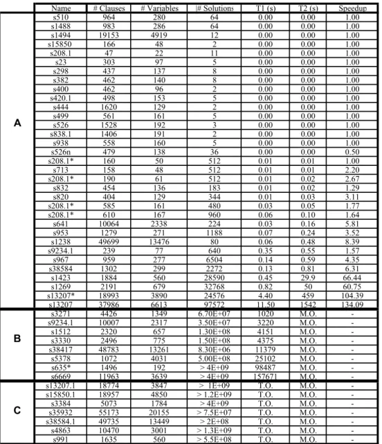
8.1
All-SAT Solver
Figure 13 shows the performance of our new All-SAT solver. The problems are CNF representations of the transition relations of the models in the benchmark. In cases where a model name is followed by ‘*’, the instance consists of multiple transitions and initial conditions. The important variables were chosen arbitrarily, and consist about half of the variables.
Group A in the table clearly shows a significant speedup for all the problems that the blocking clauses method could solve. A smaller number of clauses shortens the time of the bcp() procedure, and also allows more work to be performed in higher levels of the memory hierarchy (main memory and cache). The speedup increases with the hardness of the problem and the computation time.
Group B consists of larger instances, for which the blocking clauses method runs out of memory, yet our solver managed to complete. The number of solutions for these instances is simply too high to store in main memory as clauses. In contrast, using our new method, the solutions can be stored on the disk or in the memory of neighboring machines.
Group C in the table shows instances for which our solver timed out. In none of these cases, despite the huge number of solutions found (much larger than the size of the main memory in the machine employed), did the solver run out of memory. Our memory-efficient method clearly enables very long runs without memory blowup.
8.2
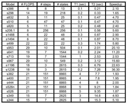
Reachability
Figure 14 shows the performance of our reachability analysis tool, calculating reach-able states of the benchmark models. Since [7] and [22] are the only reachability analysis algorithms that, as far as we know, depend solely on SAT procedures, the ta-ble shows a comparison with the performance reported in [7]. Figure 15 shows the instances for which the reachability analysis did not complete. Here, again, a compar-ison to [7] is shown. The tables show significant speedup for the completed problems, and completion of a larger number of steps for the problems not completed.
9
Conclusions
In this work we presented an efficient All-SAT engine which, unlike current engines, does not add clauses, BDDs or any other form of data, in order to block solutions already found. By avoiding the addition of this data, we gain two main advantages.
First, the All-SAT algorithm is independent of the solutions already found. There-fore, their representation can be changed, they can be processed and even deleted, without affecting the completeness of the search, or its efficiency.
Second, the memory requirements are independent of the number of solutions. This implies that, during the computation, the number of solutions already found does not
Name # Clauses # Variables |# Solutions T1 (s) T2 (s) Speedup s510 964 280 64 0.00 0.00 1.00 s1488 983 286 64 0.00 0.00 1.00 s1494 19153 4919 12 0.00 0.00 1.00 s15850 166 48 2 0.00 0.00 1.00 s208.1 47 22 11 0.00 0.00 1.00 s23 303 97 5 0.00 0.00 1.00 s298 437 137 8 0.00 0.00 1.00 s382 462 140 8 0.00 0.00 1.00 s400 462 96 2 0.00 0.00 1.00 s420.1 498 153 5 0.00 0.00 1.00 s444 1620 129 2 0.00 0.00 1.00 s499 561 161 5 0.00 0.00 1.00 s526 1528 192 3 0.00 0.00 1.00 s838.1 1406 191 2 0.00 0.00 1.00 s938 558 160 5 0.00 0.00 1.00 s526n 479 138 36 0.00 0.00 0.50 s208.1* 160 50 512 0.01 0.01 1.00 s713 158 48 512 0.01 0.01 2.20 s208.1* 190 61 512 0.01 0.02 2.67 s832 454 136 183 0.01 0.02 1.29 s820 404 129 344 0.01 0.03 3.11 s208.1* 585 161 480 0.03 0.05 1.77 s208.1* 610 167 960 0.06 0.10 1.64 s641 10064 2338 224 0.03 0.16 5.81 s953 1279 271 1188 0.07 0.24 3.52 s1238 49699 13476 80 0.06 0.48 8.39 s9234.1 239 77 640 0.35 0.55 1.57 s967 959 277 6504 0.14 0.59 4.35 s38584 1302 299 2272 0.13 0.81 6.31 s1423 1884 560 28590 0.45 29.9 66.44 s1269 2191 679 32768 0.82 50 60.75 s13207* 18993 3890 24576 4.40 459 104.39 s13207 37986 6613 97572 11.50 1542 134.09 s3271 4426 1349 6.70E+07 1020 M.O. -s9234.1 10007 2317 3.50E+07 3220 M.O. -s1512 2320 657 1.30E+08 4151 M.O. -s3330 2496 775 1.50E+08 4375 M.O. -s38417 48783 13261 8.30E+06 11379 M.O. -s5378 1072 4031 5.00E+08 25102 M.O. -s635* 1496 192 > 4E+09 98487 M.O. -s6669 11963 3639 > 4E+09 157671 M.O. -s13207.1 18774 3847 > 1E+09 T.O. M.O. -s15850.1 18957 4850 > 1.2E+09 T.O. M.O. -s3384 5073 1784 > 4E+09 T.O. M.O. -s35932 55173 20155 > 7.5E+07 T.O. M.O. -s38584.1 49735 13449 > 2E+08 T.O. M.O. -s4863 10470 3001 > 1.3E+09 T.O. M.O. -s991 1635 560 > 5.5E+08 T.O. M.O. -C
B A
Figure 13:All-SAT solving time. T1 - The time required for our new All-SAT solver. T2 - The time required for the blocking clauses-based algorithm. M.O. - Memory Out. T.O. - Time out (48 hours) Speedup - The ratio T2/T1.
become a parameter of complexity in finding further solutions. It also implies that the size of the instance being solved fits in smaller and faster levels of the memory hierarchy. As a result, our method is faster than blocking clauses based methods, and can solve instances that produce solution sets too large to fit in the machine’s memory. Our All-SAT engine uses Chaff [23] as its base code, and experimental results show significant speedup compared to the blocking clauses method used so far for this purpose. Moreover, our tool can cope with large instances which caused memory blowup when using the blocking clauses method. We applied our tool on even harder problems, which it did not complete solving. These runs were stopped after a timeout
Model # FLOPS # steps # states T1 (sec) T2 (sec) Speedup s386 6 8 13 0.1 0.21 2.10 s298 14 19 218 0.2 0.33 1.65 s832 5 11 25 0.1 0.47 4.70 s510 6 47 47 0.1 0.47 4.70 s820 5 11 25 0.2 0.48 2.40 s208.1 8 256 256 0.1 0.56 5.60 s1488 6 22 48 0.3 0.87 2.90 s1494 6 22 48 0.1 0.87 8.70 s499 22 22 22 0.3 1.74 5.80 s953 29 10 504 0.1 2.01 20.10 s641 19 7 1544 0.2 2.24 11.20 s713 19 7 1544 1 2.53 2.53 s967 29 10 549 0.2 3.12 15.60 s1196 18 3 2615 0.3 6.79 22.63 s1238 18 3 2615 0.2 7.26 36.30 s382 21 151 8865 4 7.7 1.93 s400 21 151 8865 4 7.8 1.95 s444 21 151 8865 4 8 2.00 s526n 21 151 8868 5 9.21 1.84 s526 21 151 8868 5 9.35 1.87 s349 15 7 2625 3 14.8 4.93 s344 15 7 2625 3 15.3 5.10
Figure 14: Reachability Analysis Performance. #FLOPS is the number of flip-flops in the model. #states is the total number of reachable states. T1 is the time required for our tool. T2 is the time as given in [7] using 1.5Ghz dual AMD Athlon CPU with 3GB RAM.
Actual time for max depth (sec) Max depth Completed Time to reach Depth 1 (sec) Depth 1 [7] (1000 sec') #FLOPS Model 9 1 9 1 37 S1269 580 4 25 3 74 S1423 120 3 8 2 669 S13207 2980 23 64 4 57 S1512 23853 111 291 8 228 S9234 7793 7 180 5 597 S15850 1921 4 1 2 1452 S38584
Figure 15: Reachability Analysis Performance. ‘Depth 1’ is the maximal depth reached in [7] with timeout of 1000 seconds. ‘Time to reach Depth 1’ is the time required for our tool to complete the same depth. The ‘Max depth’ and the ‘Actual time to reach max depth’ are the maximal steps successfully completed by our tool, and the time required for it. The timeout is generally 3600 seconds (1 hour), with longer timeouts for s1512, s9234 and s15850.
of 48 hours. Our solver did not run out of memory in any of these cases.
We have demonstrated how to use our All-SAT engine for quantifiers elimination in image computation. By assigning the next state model variables to be the important variables in our All-SAT solver, we eliminate all the quantifiers on the current state and input variables. The result is a memory-efficient reachability computation, based solely on SAT procedures. This reachability tool proved to reach deeper in the reachability analysis compared to other tools based only on SAT procedures, and showed significant speedup on many problems.