Simultaneous Multislice Functional Magnetic Resonance Imaging.

(1)

Simultaneous Multislice

Functional Magnetic Resonance Imaging

by

Alan Chu

A dissertation submitted in partial fulfillment of the requirements for the degree of

Doctor of Philosophy (Biomedical Engineering) in the University of Michigan

2016

Doctoral Committee:

Professor Douglas C. Noll, Chair Professor Jeffrey A. Fessler

Assistant Research Scientist Jon-Fredrik Nielsen Associate Research Scientist Scott J. Peltier

(2)

©Alan Chu 2016

(3)

Acknowledgments

First and foremost, I’d like to thank Doug Noll for accepting me as a student and providing many years of help and guidance. He has incredible intuition in medi-cal imaging, which translates to great teaching and clear explanations of very com-plex concepts. I was extremely fortunate to be able to learn from him. From a non-scientific standpoint, he also has exceeded all expectations I’ve had for a great mentor; even though he has accomplished so much in the medical imaging world, he understands the importance of a good work-life balance. Although busy, he makes it a priority to meet with his students and is always friendly and passionate about our work. In addition, he has been incredibly supportive of my clinical medicine pursuits. I’d also like to thank the rest of my committee for helping me with research throughout the years. Jeff Fessler has been amazing in helping me understand image reconstruction better, and I was lucky to be able to learn from such an expert in the field. When I first joined the lab, Jon Nielsen was the one who taught me pulse sequence development on our scanner and has continued to provide great expertise in various different areas in MRI over the years. Scott Peltier has also provided tremendous help to me; he was the one I always went to in order to ensure my subject scans were done properly and if any scanner issues came up.

My fellow U of M fMRI Lab members, both past and present, also deserve a huge thanks for answering all the questions I asked them, and making imaging research more fun. Luis Hernandez-Garcia was always great for bouncing ideas off of, and his great sense of humor always brightens my day. Daehyun Yoon, Hesam Jahanian, and Yoon Chung Kim were the senior students when I first started out in

(4)

the lab and helped me tremendously when I was first learning the basics of MRI. I was also lucky to learn from someone as smart and incredibly productive as Feng Zhao. Matt Muckley definitely made lab life more fun. I can always count on him to provide great conversation on a wide array of topics such as beer, world history, and image reconstruction, just to name a few. Hao Sun is another super smart and productive member of our lab, and I learned a lot from him. The rest of the lab, including Kathleen Ropella, Sydney Williams, and Tianrui Luo, has also been a pleasure to work with. I’d also like to thank members of Jeff’s lab: Mai Le, whom I had great times with during EECS 556, Gopal Nataraj, and Dan Weller.

Finally, I’d like to thank my family for their support and encouragement. My sister Alina always believes in me no matter what the odds are of success. Pete taught me what the important things are in life and made every day a better one with his good nature, loyalty, and infinite patience. I’ll always miss him. Last but definitely not least, I thank my parents, Jason and Kathy Chu, for supporting me throughout my life. This work would not have been possible without their unwavering love and guidance. Any success I’ve had or will have in the future is because of them.

(5)

LIST OF FIGURES

2.1 Example RF pulse for a 3 simultaneous slice acquisition created from a

6.4 ms Hamming-windowed sinc with 4 zero-crossings. . . 6

2.2 Slice profiles for Hadamard-encoded fMRI with 2 simultaneous slices. . . 10

2.3 Two simultaneous slice acquisitions with no readoutz-gradient (top row),

and a blipped-CAIPI readout z-gradient (bottom row). The SMS

ac-quisition is shown in the right column, which is simply the sum of the individual slices shown in the left and middle columns. . . 16

2.4 Slice profile for a 3 simultaneous slice acquisition created from the 6.4 ms

Hamming-windowed sinc with 4 zero-crossings shown in Figure 2.1. . . . 17

2.5 Slice-GRAPPA kernel operation to compute thek-space data for one coil of one separated slice. Each kernel operates on all coils of the SMSk-space data.. . . 21

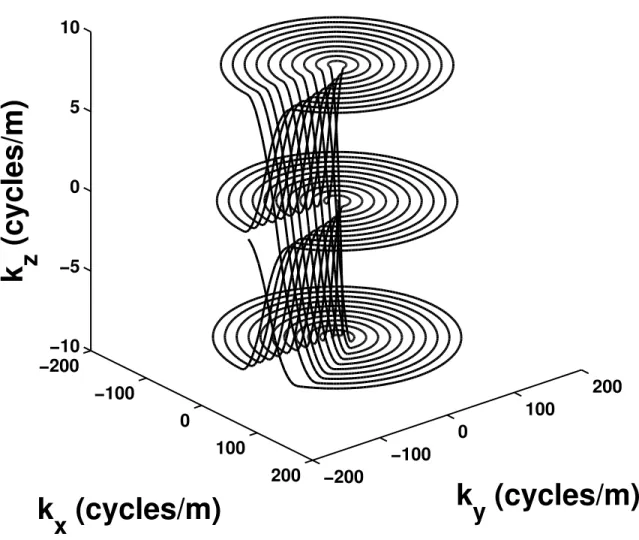
2.6 Three-dimensional blipped spiral k-space trajectory for a 3 simultaneous slice acquisition. . . 23

3.1 SNRHada/SNRconv described by Equation (3.7) when reconstructing the slices by filtering the squared magnitude of the data. Assuming no noise correlation between subslices, this is also the SNR ratio when reconstruct-ing slices by separatreconstruct-ing subslices first, then combinreconstruct-ing. Typical values of λ = 0.008 and SNR0 = 100 from Ref. [54] are used. The plane at

SNRHada/SNRconv = 1 is shown for illustration. A significant portion of the plot is below 1, indicating an SNR disadvantage for Hadamard-encoding for those values of cand ∆θ. . . 30

3.2 Example phase time series for one non-separated voxel of a

Hadamard-encoded fMRI scan with two simultaneously acquired slices. . . 34

3.3 Frequency and step response of the low-pass Parks-McClellan FIR filter

used to extract the simultaneous slices in Hadamard-encoded fMRI. The filter is 17 taps long, and the sampling frequency of the fMRI scan is

Fs = 1 Hz. . . 36

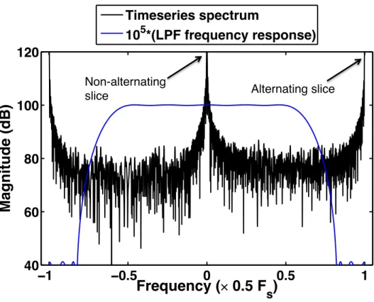
3.4 Example magnitude spectrum of a non-separated voxel time series in

Hadamard-encoded fMRI with two simultaneous slices. In this work, the

(9)

3.5 Activation maps over reconstructed images for run 1 of a Hadamard-encoded scan of subject 3, with (top) and without (bottom) physiological noise correction. A visual and motor block paradigm was used. The underlying background image is the actual result using the Hadamard reconstruction process described in Section 3.2. A t-score threshold of 4 was used. . . 41

3.6 Activation maps over reconstructed images for run 1 of a conventional

non-SMS scan of subject 3, with (top) and without (bottom) physiologi-cal noise correction. A visual and motor block paradigm was used. The underlying background image is the actual result using the non-SMS re-construction process described in Section 3.2. At-score threshold of 4 was used.. . . 42

3.7 Mean ROC curve across all 10 subjects for each method. ROC curves

were generated with t thresholds from 0 to 7 in increments of 0.5, then linearly interpolated to false detection probability steps of 1×10−6, then averaged across subjects. . . 44

3.8 Mean ROC curve across all 10 subjects for each method. This plot is

the same as Figure 3.7, except zoomed-in to a more practical range of 4.8×10−5 to 0.04 for the probability of false detection. ROC curves were generated with tthresholds from 0 to 7 in increments of 0.5, then linearly interpolated to false detection probability steps of 1×10−3_{, then averaged}

across subjects. . . 45

3.9 For each method, this figure plots the mean area under the ROC

curve across all 10 subjects for false detection probabilities ranging from 4.8×10−5 to 0.04. A range around each mean is also plotted, where each range is equivalent to one-half the 95% confidence interval for the differ-ence between estimated group means computed from the Tukey multiple comparison procedure. If the ranges for two methods overlap, there is no significant difference in mean areas, and equivalently, the p-value is greater than 0.05. If the ranges for two methods do not overlap, there is a significant difference in mean areas, and equivalently, the p-value is less than 0.05. . . 48

4.1 Sine wavegz(t) modulated spiral k-space trajectory used for 3

simultane-ous slices. . . 56

4.2 Different views of the trajectory in Figure 4.1. . . 56

4.3 (a) kx-ky components of the concentric ring k-space trajectory used in

this work. Boundaries of angular sectors for GRAPPA are shown with dash-dotted blue lines. (b) Close-up of ring transitions with “x” markers indicating where samples were acquired. . . 61

4.4 Three-dimensional concentric ringk-space trajectory for a nslc = 3 simul-taneous slice acquisition. . . 62

4.5 Readout gradient waveforms used to produce anslc = 3 simultaneous slice

concentric-ring-in trajectory. The x and y gradients were designed using the numerical algorithm described in Section 4.1.6. . . 63

(10)

4.6 Non-Cartesian slice-GRAPPA using blipped concentric rings. The tra-jectory is unwinded into a Cartesian grid and divided into sectors before kernel operations are performed. . . 65

4.7 Spiral SMS simulations: SENSE method reconstructions of 3 different

slices of a phantom. Non-SMS SENSE reconstruction shown in (a). SMS reconstruction without gz(t) modulation shown in (b), with blipped gz(t)

modulation shown in (c), with regularization using Equation (4.2) and blipped gz(t) modulation shown in (d), with sine wave gz(t) modulation

shown in (e), and with regularization using Equation (4.2) and sine wave

gz(t) modulation shown in (f). On the right, (g), (h), (i), (j), and (k) are the absolute difference images of (b), (c), (d), (e), and (f), respectively, with (a). . . 71

4.8 Coil sensitivities of the 8-channel Invivo head coil used for the spiral SMS simulations and experiments. Top row shows coil 1, middle row shows coil 4, and bottom row shows coil 7. Three different slices corresponding to the slices in Figure 4.7 are shown across the columns. . . 72

4.9 All reconstructions using all β combinations for the blipped spiral SMS simulation with regularization in Equation (4.2). (a) shows the recon-struction using β1 = 273, β2 = 5, and β3 = 5, where slice 1 refers to the image on the left, slice 2 is the center image, and slice 3 is the image on the right. (b) shows the reconstruction using β1 = 5, β2 = 273, and β3 = 5. (c) shows the reconstruction using β1 = 5, β2 = 5, andβ3 = 273. (e), (f), and (g) are the absolute difference images of (a), (b), and (c), re-spectively, with the original non-SMS slices used in the simulation, which are shown in Figure 4.7(a). (d) shows the reconstruction for the blipped spiral SMS simulation using traditional regularization with a singleβ, and is the same as the image in Figure 4.7(c). (h) is the difference image of (d), and is the same as the image in Figure 4.7(h). . . 73

4.10 Modulation PSF using blipped-CAIPI. . . 76

4.11 Spiral SMS: modulation PSF for a slice 39 mm away from isocenter using a blippedgz(t) in (b), and using the sine wavegz(t) in (c). The point used to computed the modulation PSFs is shown in (a) and has a magnitude of 90. The maximum magnitude in the center of (b) and (c) is approximately 10.09 and 47.1, respectively. The modulation waveforms are specified in Section 4.1.1 and Section 4.1.4. . . 76

4.12 Spiral SMS: modulation pattern for a brain slice 39 mm away from isocen-ter using a blipped gz(t) in (b), and using the sine wave gz(t) in (c). Instead of a point, the brain image shown in (a) was used to compute the images in (b) and (c). The modulation waveforms are specified in Section 4.1.1 and Section 4.1.4. . . 77

(11)

4.13 Spiral SMS experiments: SENSE method reconstructions of 3 different slices of a phantom. Non-SMS reference for blipped gz(t) shown in (a).

SMS reconstruction with blippedgz(t) modulation shown in (b), with

reg-ularization using Equation (4.2) and blipped gz(t) modulation shown in

(c). Non-SMS reference for sine wavegz(t) shown in (d). SMS

reconstruc-tion with sine wavegz(t) modulation shown in (e), and with regularization

using Equation (4.2) and sine wave gz(t) modulation shown in (f).. . . . 78

4.14 All reconstructions using all β combinations for blipped spiral SMS ex-periment with regularization in Equation (4.2). Top row shows the re-construction using β1 = 273, β2 = 5, and β3 = 5. Middle row shows the reconstruction using β1 = 5, β2 = 273, and β3 = 5. Bottom row shows

the reconstruction using β1 = 5,β2 = 5, and β3 = 273. The images in the

left column are slice 1, the images in the center column are slice 2, and the ones on the right column are slice 3. . . 79

4.15 Sensitivity maps of the isocenter slice using the Nova Medical 32-channel receive head coil used for the concentric ring scans in this work. . . 80

4.16 Concentric ring simulations: reconstruction results for SENSE, SG, and SP-SG, as well as the non-SMS slices used to create SMS data in the simulations. The separated, non-SMS slices are numbered consecutively from 1 to 39 starting most inferiorly and going superiorly. The number at the top of each column of images indicates the slice number for that column. . . 87

4.17 Concentric ring simulations: absolute difference images between each re-construction method labeled on the left and the non-SMS slices used to simulate the SMS acquisition. The non-SMS slices used as the “truth” are the ones shown in Figure 4.16 labeled “non-SMS.” The number at the top of each column of images indicates the slice number for that column. 88

4.18 Concentric ring simulations: using each method, the top 3 plots show the RMSE within individual slices. The bottommost plot shows the RMSE for each acquisition of 3 simultaneous slices shown directly above it in the upper 3 plots. . . 89

4.19 Concentric ring simulations: field maps used for the reconstructions. The number at the top of each column of images indicates the slice number for that column. The colormap is in units of Hertz. . . 90

4.20 (a) Point used to calculate the modulation PSF using blipped spirals (b), and using blipped concentric rings (c). The magnitude of the point in (a) is 90. The maximum magnitude at the center in (b) and (c) is approximately 10.09 and 4.28, respectively. . . 91

4.21 Same modulation PSFs shown in Figure 4.20, except windowed lower to portray the differences at the center more clearly. Image (a) shows the point used to calculate the modulation PSF using blipped spirals (b), and using blipped concentric rings (c). The magnitude of the point in (a) is 90. The maximum magnitude at the center in (b) and (c) is approximately 10.09 and 4.28, respectively. . . 92

(12)

4.22 Modulation pattern resulting from a blipped concentric ring trajectory for 3 simultaneous slices. The numbers at the top indicate the slice num-ber, where contiguous slices in the volume are numbered 1 through 39. The 20th slice is acquired at z-isocenter, assuming an axial acquisition. The top row shows the original, non-modulated, 3 simultaneous slices. The bottom row shows what the blipped modulation does to the various slices. Slice 20 is unaffected because it is acquired at z-isocenter. The blipped EPI equivalent of slices 7 and 33 would be a simple FOV shift. The modulation pattern for all acquisitions in the volume are shown in Figure 4.23. . . 93

4.23 Modulation pattern resulting from a blipped concentric ring trajectory for 3 simultaneous slices. The numbers at the top indicate the slice number, where contiguous slices in the volume are numbered 1 through 39. The 20th slice is acquired at z-isocenter, assuming an axial acquisition. The top row in each of (a), (b), and (c) shows the original, non-modulated slices. The bottom row in each of (a), (b), and (c) shows what the blipped modulation does to the various slices. Each column of images in (a), (b), and (c) form the set of images acquired simultaneously in a 3 simultaneous slice acquisition. The acquisition consisting of slices 7, 20, and 33 is shown in Figure 4.22. . . 94

4.24 Activation map of a 3 simultaneous slice concentric ring fMRI scan with a visual stimulus and motor task. The underlying grayscale image is the SP-SG reconstruction result for one time frame in the middle of the scan. The colormap is the t-score. . . 95

4.25 Sine wavegz(t) sampling pattern in thekx-ky plane at kz =kmax_z ≈12.821 m-1_{. This plot is essentially a slice through the top edge of Figure 4.1.} _. ₉₅

5.1 Illustration showing the concept of interslice leakage artifacts (top two rows), intraslice artifacts (third row), and total image artifacts (bottom row). In this figure, wv indicates the kernel that computes k-space data

of (one coil of) separated slicev. . . 107

5.2 (a) Activated voxel counts: mean across all 5 subjects. (b) Normalized

activated voxel counts: mean across all 5 subjects with error bars indicat-ing 95% confidence intervals. Before takindicat-ing the mean across subjects, the count for each method was normalized by the count using all 32 coils. (c) Falsely activated voxel counts: mean across all 5 subjects. Falsely acti-vated voxels are defined as active brain voxels that are outside the visual and motor cortex areas used for the activated voxel counts in (a) and (b). A t-score threshold of 6 was used for all methods. . . 110

(13)

5.3 (a) Visual and (b) motor cortex activation maps over reconstructed images for subject 5. The underlying background image is the actual result using the indicated reconstruction method. A t-score threshold of 6 was used for all methods. The top of each column lists the number of virtual coils for that column. For each of (a) and (b), the same visual or motor cortex slice is pictured for all methods and number of virtual coils. The activated voxel color scale is the t-score.. . . 113

5.4 Virtual coil sensitivities for slice 20, thez-isocenter slice, when computing the compression matrices from (a) the non-SMS data and (b) the SMS data for 10 virtual coils. . . 114

5.5 (a) Interslice leakage artifact metric (L2→1+L2→3), (b) intraslice artifact

metric (I2→2 −I2), and (c) total image artifact metric (L1→2 +I2→2 + L3→2−I2) for the middle slices of a 3-simultaneous-slice-acquired volume

of 39 total axial slices. All methods used a concentric ring trajectory except for the “Spiral SENSE” method. . . 115

5.6 (a) Interslice leakage artifact for the inferior slice (L2→1), (b) intraslice

artifact for the middle slice (I2→2−I2), and (c) interslice leakage artifact

for the superior slice (L2→3) from the middle slice of a 3 simultaneous slice

acquisition. The image on the right shows the ground truth inferior (a), middle (b), and superior (c) slices. All methods used a concentric ring trajectory except for the “Spiral SENSE” method. . . 116

5.7 Average retained SNR, or equivalently, average 1/g-factor within brain voxels. All methods used a concentric ring trajectory except for the “Spi-ral SENSE” method. . . 119

5.8 Maps of retained SNR, or equivalently, 1/g-factor of the same slices used in Figure 5.6. (a) Inferior slice, (b) middle slice, and (c) superior slice. All methods used a concentric ring trajectory except for the “Spiral SENSE” method. . . 120

5.9 (a) Maps of retained SNR, or equivalently, 1/g-factor without demodu-lating non-z-isocenter acquisitions prior to SP-SG reconstruction (with no coil compression). Each column of 3 images is the retained SNR map for a single acquisition of 3 simultaneous slices. The number at the top of each column indicates the acquisition number, where acquisition 7 is at z-isocenter and acquisition 1 and 13 are the furthest from isocenter. (b) Maps of retained SNR with appropriate demodulation prior to SP-SG reconstruction (with no coil compression). . . 121

5.10 Reconstruction times of the first time frame of fMRI scans of subject 5. The time needed for field map, sensitivity map, and GRAPPA kernel generation is not included in these reconstruction times. The time needed for coil compression is included. . . 122

(14)

5.11 This plot displays the complex sum across nslc = 3 consecutive rings,

assuming each ring has a total magnitude of 1 and the phase of each ring only depends on the blipped readout z-gradient and the slice location. Acquisition 7 occurs with the middle slice atz-isocenter, and acquisitions 1 and 13 are the furthest away from isocenter. For each acquisition, the sum across the nslc = 3 simultaneous slices is also plotted and is equal to

3. Note that for acquisition 7 at z-isocenter, the middle slice has a value the furthest away from the inferior and superior slices. . . 129

5.12 In conventional coil compression, Vcomp is computed from the SMS k

-space data, which is the sum of 3 slices spatially separated far apart from each other. Before sensitivity maps are computed or kernel calibration is performed, each non-SMS slice is compressed using the same Vcomp. In

GRABSMACC, Vcomp is computed from the non-SMS k-space data. For

sensitivity maps or kernel calibration, each non-SMS slice is compressed using adifferent Vcomp that is tailored for that specific slice. . . 131

(15)

LIST OF TABLES

3.1 Area under the ROC curve for false detection probabilities ranging from

4.8 × 10−5 to 0.04 for each subject and method. “Hada” indicates

Hadamard-encoded fMRI, “Hada Physio” indicates Hadamard-encoding with physiological noise correction, and similarly for “Conv” and “Conv Physio” for conventional, non-SMS fMRI. . . 46

3.2 This table displays p-values using paired Tukey multiple comparisons of

a two-way ANOVA of areas under the ROC curves displayed in Table 3.1. 47

4.1 For each method, this table shows the RMSE for each of the

individ-ual slices, as well as the combined RMSE for all 3 slices in the spiral SMS simulation. The SENSE reconstruction of the non-SMS image in Figure 4.7(a) is used as the true image. . . 74

5.1 For each method, this table displays p-values using paired Dunnett mul-tiple comparisons of a two-way ANOVA of activated voxel counts. The count for each number of virtual coils is compared pairwise with the count using all 32 coils using the same method. For each method, the value in bold corresponds to the largest number of virtual coils with a p-value less than 0.05, or equivalently, the largest number of virtual coils with an activation count that differs significantly from the non-compressed recon-struction. . . 112

5.2 Assuming that each ring has a total magnitude of 1, and that the phase

for each ring is only dependent on gz and the slice location, this table

plots the complex value for each ring and slice for acquisition 1, which is the furthest away from z-isocenter and consists of slices 1, 14, and 27. The sum across the 3 rings is also shown for each slice. . . 128

(16)

ABSTRACT

Simultaneous Multislice Functional Magnetic Resonance Imaging

by

Alan Chu

Chair: Douglas C. Noll

Functional magnetic resonance imaging (fMRI) is a valuable tool for mapping brain activity in many fields. Since functional activity is determined by temporal signal changes, undesired fluctuations from physiological motion are problematic. Simul-taneous multislice (SMS) imaging can alleviate these issues by accelerating image acquisition, increasing the temporal resolution. Furthermore, some applications re-quire a temporal resolution higher than what conventional fMRI will allow. Current research in SMS has focused on Cartesian readouts due to their ease in analysis and reconstruction. However, non-Cartesian readouts such as spirals have shorter readout times and better signal recovery.

This work explores the acquisition and reconstruction of both spiral and concentric ring readouts in parallel SMS. The concentric ring readout retains most of the bene-fits of spirals, but also increases the usability of alternative reconstruction techniques for non-Cartesian SMS such as generalized autocalibrating partially parallel acquisi-tions (GRAPPA). To date, non-Cartesian SMS imaging has only been reconstructed

(17)

reconstructions have reduced root-mean-square-error compared to SENSE and good subjective image quality as well. Furthermore, using point spread function analysis, the concentric ring trajectory is found to have superior slice separation properties compared to a spiral one.

Since parallel imaging greatly magnifies the amount of data used for reconstruc-tion, a novel coil compression method is developed, which outperforms conventional coil compression in fMRI, substantially decreasing the amount of reconstruction time needed for sufficient detection of functional activation. Results indicate that the pro-posed method can compress 3 simultaneous slice data using a 32-channel coil down to only 10 virtual coils without any adverse effects in functional activation, noise, or image artifacts. Competing methods require substantially more coils for preservation of the data, resulting in large reconstruction time savings for the proposed method.

This work also explores the use of Hadamard-encoded fMRI for increased tempo-ral resolution. Because Hadamard-encoded SMS uses data from multiple time frames to separate slices, physiological noise correction is critical. However, even with phys-iological noise correction, results indicate Hadamard-encoded fMRI is not as reliable as conventional fMRI due to undesired temporal fluctuations, most notably from uncorrected physiological noise.

(18)

CHAPTER 1 Introduction

Functional magnetic resonance imaging (fMRI) has become the prevailing method for non-invasively mapping human brain activity. The technology is widely used in neuroscience and psychology to evaluate models of cognition and in clinical medicine to develop biomarkers for neurological and psychiatric diseases. In neurosurgery, fMRI has been increasingly used to help identify critical brain regions in patients prior to brain tumor or seizure foci resection.

In fMRI, standard clinical magnetic resonance imaging (MRI) scanners are used to repetitively acquire images of the brain over an interval of time lasting several minutes. These images track small changes in the brain that correlate with a stimulus or task the subject is instructed to perform during the scan. The majority of fMRI scans use blood oxygenation level dependent (BOLD) contrast, which uses the content of deoxyhemoglobin in the blood as the contrast agent [1]. As the subject performs the task or is exposed to the stimulus, active regions of the brain will have increased blood flow [2, 3], which decreases the concentration of deoxygenated hemoglobin in that region [4]. Deoxygenated hemoglobin causes transverse dephasing in the signal relative to oxygenated hemoglobin, so a decrease in deoxygenated hemoglobin results in decreased dephasing and an increased signal intensity. In other words, increased blood flow to active brain regions causes a decrease in deoxygenated hemoglobin, which changes the magnetic susceptibility of the blood, leading to a signal intensity

(19)

Since functional activity in fMRI is determined by temporal changes in the signal, cardiac pulsations and respiratory motion can corrupt the resulting functional activity maps because they also cause significant temporal fluctuations in the acquired fMRI signal [8,9,10,11,12]. In a typical fMRI scan, one whole-brain volume is acquired in approximately 2 seconds, resulting in a frame rate of around 0.5 Hz. This sampling rate is high enough for typical task-based fMRI experiments responsible for capturing functional paradigms occurring at around 0.02 to 0.06 Hz. However, human resting heart rates are usually around 1.0 to 1.6 Hz, and the resulting noise can alias down into the frequency of interest. In addition, motion from respiration can also create noise at 0.2 to 0.3 Hz. Similar to task-based fMRI, signal fluctuations occurring at frequencies less than 0.1 Hz are of interest in resting state fMRI. However, in resting state fMRI, the paradigm waveform is not known a priori; the acquired data is itself used to determine correlations between regions of the brain. Thus, physiological noise present in the data can spuriously increase or decrease the apparent correlation between two time courses. Methods have been developed to correct for physiological noise in fMRI including post-processing methods [13,14,15,16] and navigator-based methods [12,17]. More recently, work has been done to model respiration and cardiac fluctuations by developing impulse response functions [18, 19]. Regardless of the method used, accelerated fMRI acquisitions with a higher temporal resolution can increase the effectiveness of physiological noise correction. In addition, the increase in time points provides for greater statistical power in the data [20], and more options for bulk head motion correction.

Simultaneous multislice (SMS) imaging, also called multiband imaging, is a method that can be used to accelerate fMRI by acquiring multiple slices simulta-neously, thereby covering the same region as a conventional acquisition in a smaller amount of time. Because the slices are acquired simultaneously, the raw data contains overlapped or aliased images, which must be separated during the image

(20)

reconstruc-tion process.

1.1 Aims

In Chapter2, basic principles behind MRI are introduced in order to understand how SMS imaging works and why SMS imaging is potentially an excellent technique for accelerating fMRI. Existing methods for SMS imaging are covered, including both non-parallel and parallel SMS imaging methods.

In Chapter 3, Hadamard-encoded SMS fMRI is explored. Hadamard-encoded imaging is an SMS imaging method that does not require multiple coils in order to separate the simultaneous slices. This work aims to further develop Hadamard-encoded imaging for fMRI by evaluating the temporal resolution and SNR benefits in human subject scans.

Chapter 4 investigates parallel SMS fMRI using non-Cartesian readout trajec-tories. Spiral parallel SMS imaging is improved by further optimizing the readout z-gradient waveform along with the kx-ky trajectory, by developing improved

recon-struction techniques in both the image and k-space domains, and by demonstrating practical utility in fMRI studies.

In parallel SMS imaging, the amount of acquired data is multiplied by the number of receive coils used, which represents a significant increase in the computational load during reconstruction. In Chapter 5, a novel SMS coil compression method is developed to reduce the time needed for reconstruction while preserving functional activation and image quality. The method is compared with existing methods in SMS imaging as well as with conventional non-SMS imaging.

Final remarks regarding the work presented in this dissertation are included in Chapter 6, along with a description of the contributions made and potential avenues for future work.

(21)

CHAPTER 2 Background

2.1 Two-dimensional and Three-dimensional MRI

In MRI, the complex signal acquired in coil u is

su(t) =

Z Z Z _h

cu(x, y, z)m(x, y, z)e−t/T2(x,y,z)

e−i2π(kx(t)x+ky(t)y+kz(t)z+∆f0(x,y,z)t)i_d_x_d_y_d_z,

(2.1)

where m(x, y, z) is the three-dimensional object as a function of spatial position (x, y, z), cu(x, y, z) is the sensitivity of coil u to location (x, y, z), T2(x, y, z) is

the transverse relaxation time constant of the object, ∆f0(x, y, z) is the

spatially-dependent B0 inhomogeneity, t is time, and k(t) = ₂γ_π

Rt

0 g(τ) dτ, where γ is the

gyromagnetic ratio, and g(t) is the spatially-dependent magnetic field gradient as a function of time. For the sake of simplicity in this dissertation, we will ignore the relaxation terme−t/T2(x,y,z) _{in Equation (}_2.1_).

In conventional multislice imaging, a single two-dimensional slice is acquired with each excitation and no z-gradient is used during readout. Setting kz(t) = 0,

assum-ing infinitely thin slices, and arbitrarily assignassum-ing x and y to denote the in-plane dimensions, the signal equation becomes

su(t) =

Z Z

(22)

for two-dimensional MRI. In reality, however, slices cannot be infinitely thin, so the summation over z in Equation (2.1) still occurs. This can lead to signal loss from through-plane dephasing.

Standard fMRI typically uses a single-shot, two-dimensional approach, where in-dividual slices are acquired sequentially to provide whole-brain coverage in approxi-mately 2 seconds. Given a desired spatial resolution, the minimum repetition time (TR) is limited by the number of slices. Conventional parallel imaging [21,22,23] has been demonstrated to successfully accelerate multislice MRI scans in-plane. These methods all use multiple receive coils to allow for undersampling of k-space within each slice. However, the amount of acceleration is limited with conventional parallel imaging in fMRI because of the need for an appropriate echo time (TE) for sufficient T₂∗ contrast. Three-dimensional acquisitions are another approach for acceleration in fMRI [24, 25, 26]. However, three-dimensional acquisitions require much longer readout times, which increases its vulnerability to magnetic field inhomogeneities. In addition, the readout times can stretch well beyond the TE for gray matter, depending on the desired spatial resolution and coverage.

2.2 Simultaneous Multislice MRI

Simultaneous multislice (SMS) acquisitions are yet another approach to acceleration. In SMS imaging, multiple two-dimensional slices are both excited and acquired simul-taneously, and the reconstruction process is used to separate the slices and transform the data into the image domain. If l is the number of simultaneous slices with each acquisition, and again assuming infinitely thin slices, Equation (2.1) becomes

su(t) = l X v=1 Z Z cu,v(x, y)mv(x, y)e−i2π(kx(t)x+ky(t)y+∆f0,v(x,y)t)dxdy, (2.3)

(23)

where mv(x, y) is one simultaneous slice as a function of spatial position (x, y) and

cu,v(x, y) is the sensitivity of coil u to simultaneous slice v. Note that SMS imaging

does not necessarily require multiple receive coils. When only one coil is used, the coil index uis removed from Equation (2.3) and the coil sensitivitycv(x, y) is assumed to

be 1.

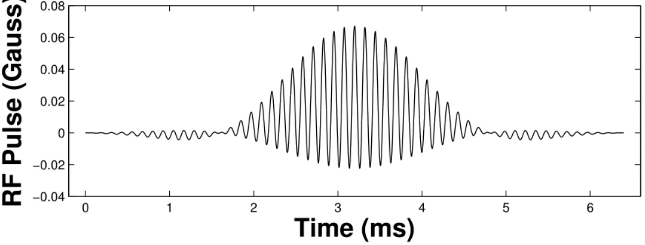
The simultaneous slices are excited using a radio frequency (RF) pulse that se-lectively tips down spins in certain planes along one particular imaging axis, usually the z-axis by convention. Using the small-tip regime[27][28], the SMS RF pulse can be implemented as a sum of l frequency-offset, Hamming-windowed sinc functions

RF(t) = l X v=1 ei2πf˜vt_sinc(_f RFt)[0.54 + 0.46 cos(2πt/T)], (2.4)

where T is the duration of the pulse, fRF is the bandwidth of the sinc, and ˜fv is

the frequency-offset for simultaneous slice v. The value of ˜fv controls how far the

simultaneous slices are from each other, and a conventional constant slice-select z -gradient with rewinder is applied during the RF pulse. Figure2.1 shows the SMS RF pulse created for a 3 simultaneous slice acquisition.

0 1 2 3 4 5 6 −0.04 −0.02 0 0.02 0.04 0.06 0.08

Time (ms)

RF Pulse (Gauss)

Figure 2.1: Example RF pulse for a 3 simultaneous slice acquisition created from a 6.4 ms Hamming-windowed sinc with 4 zero-crossings.

(24)

When SMS is applied to fMRI, multiple simultaneous-slice acquisitions are per-formed per TR to provide whole-brain coverage. Therefore, SMS imaging can be viewed as a combination of two-dimensional and three-dimensional imaging. SMS acquisitions provide an excellent avenue for acceleration in fMRI because the TE requirement does not limit the amount of acceleration as it does in conventional two-dimensional parallel imaging, and SMS does not suffer from the excessively long readout times of three-dimensional fMRI.

2.2.1 Non-parallel SMS Imaging

The earliest SMS methods did not require multiple receive coils. Souza et al. [29] developed an SMS method using Hadamard-encoded excitation as an alternative to 3-dimensional Fourier transform (3DFT) imaging. The aim was not acceleration, but to provide for more flexible slice placement over 3DFT imaging, and also to avoid the 3DFT Gibbs artifacts in the slice direction.

In Hadamard-encoded imaging of l simultaneous slices, l separate excitations are needed, each using a different RF pulse. During each excitation, the RF pulse imparts either a positive (1) or negative (-1) sign on each simultaneous slice according to a row of Hl, a Hadamard matrix of order l. For example, with an l = 2 simultaneous

slice acquisition, l = 2 different RF pulses are needed to excite the slices according to the Hadamard matrix of order 2,

H2 =    1 1 1 −1   . (2.5)

In this case, one RF pulse would need to excite both slice 1 and slice 2 with positive signs. The equation for this RF pulse is just Equation (2.4) withl = 2. The other RF pulse needs to excite one slice with a positive sign and the other one with

(25)

a negative sign. The equation of this RF pulse is RF(t) = [ei2πf˜1t_sinc(_f RFt)−ei2π ˜ f2t_sinc(_f RFt)][0.54 + 0.46 cos(2πt/T)], (2.6)

where slice 2 is the one with a negative sign. Therefore, one excitation gives a signal ¯

s1(t) = ˜s1(t) + ˜s2(t), and the other excitation gives a signal ¯s2(t) = ˜s1(t)−˜s2(t),

where ˜s1(t) is the signal from slice 1 and ˜s2(t) is the signal from slice 2. Putting these

together in a 2-element vector, we have

   ¯ s1(t) ¯ s2(t)   =    ˜ s1(t) + ˜s2(t) ˜ s1(t)−s˜2(t)   =H2    ˜ s1(t) ˜ s2(t)   =    1 1 1 −1       ˜ s1(t) ˜ s2(t)   . (2.7)

Withl = 4 simultaneous slices, 4 different RF pulses are used to produce 4 different excitations described by          ¯ s1(t) ¯ s2(t) ¯ s3(t) ¯ s4(t)          =H4          ˜ s1(t) ˜ s2(t) ˜ s3(t) ˜ s4(t)          =          1 1 1 1 1 −1 1 −1 1 1 −1 −1 1 −1 −1 1                   ˜ s1(t) ˜ s2(t) ˜ s3(t) ˜ s4(t)          . (2.8)

For any Hadamard matrix, (1_l)H_l∗Hl =Il. Therefore, to separate the slices, simply

perform the matrix multiplication

            ˜ s1(t) ˜ s2(t) ˜ s3(t) ˜ s4(t) .. .             = 1 l H_l∗             ¯ s1(t) ¯ s2(t) ¯ s3(t) ¯ s4(t) .. .             . (2.9)

(26)

trans-formation into the image domain can be performed, ideally with B0 inhomogeneity

correction. It is also possible to perform the transformation into the image domain first, then add and subtract the aliased slices using the Hadamard matrix to separate them.

Hadamard-encoded SMS was later extended to fMRI for the purposes of reduced signal dropout from susceptibility-induced gradients [30]. In that work, 2 simulta-neous “subslices” were acquired using Hadamard-encoding and compared to a con-ventional acquisition consisting of a non-SMS acquisition with slice thickness twice that of each individual Hadamard subslice. The idea is that the thinner subslices us-ing Hadamard-encodus-ing will have reduced signal dropout from susceptibility-induced field gradients, but since 2 subslices are excited simultaneously, the accompanying SNR loss from the thinner subslices is avoided. However, this is done at the expense of temporal resolution.

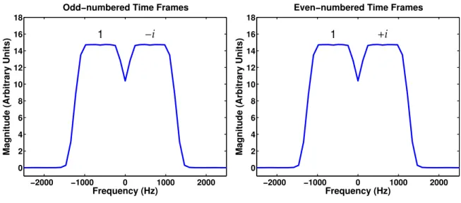
In Ref. [30], instead of encoding each subslice with a +1 or −1 sign, every other subslice is encoded with a±1 or±imultiplication. For example, with 4 simultaneous subslices, the Hadamard-encoding matrix is

H4 =          1 i 1 i 1 −i 1 −i 1 i −1 −i 1 −i −1 i          .

This is done so that the transition zones of the slice profiles do not vary from time frame to time frame, as shown in Figure 1 of Ref. [30], which results in more uniform slice profiles after reconstruction. For 2 simultaneous subslices, the encoding would just alternate between 1 +i and 1−i from frame to frame, as shown in the slice profiles plotted in Figure 2.2.

(27)

−2000 −1000 0 1000 2000 0 2 4 6 8 10 12 14 16 18 Frequency (Hz)

Magnitude (Arbitrary Units)

1

Odd−numbered Time Frames −i −2000 −1000 0 1000 2000 0 2 4 6 8 10 12 14 16 18 Frequency (Hz)

1

Even−numbered Time Frames +i

Figure 2.2: Slice profiles for Hadamard-encoded fMRI with 2 simultaneous slices. In Ref. [30], simultaneously acquired subslices are modeled as

In =eiφ M

X

m=1

Sm,neiθm, (2.10)

where n is the time frame number, Sm,n is the magnitude of the mth subslice, θm

is the phase difference between subslices arising from the susceptibility-induced field gradients, andφis an overall phase shift. For 2 simultaneous subslices, a conventional acquisition is just

I_nconv =eiφ(S1,n+S2,nei∆θ),

where ∆θ is the phase difference between subslices. The magnitude of the signal is

|I_nconv|=

q

S2

1,n+S22,n+ 2S1,nS2,ncos ∆θ. (2.11)

The Hadamard-encoded signal is modeled as

(28)

making the magnitude

|I_nHada|=

q

S2

1,n+S22,n−2(−1)nS1,nS2,nsin ∆θ. (2.13)

Since the goal is to reduce signal dropout and not necessarily to recover the individual subslices, the authors propose the reconstruction process of low-pass filtering|IHada

n |2

to get the time series

xn=

p

F−1_{_W

nF(|InHada|2)}, (2.14)

where F is the Fourier transform operator, and Wn is the spectrum of the low-pass

filter. The low-pass filter removes the−2(−1)n_S

1,nS2,nsin ∆θ term in Equation (2.13)

to obtain

xn=

q

S2

1,n+S22,n. (2.15)

Numerous other non-parallel methods have been created for SMS imaging. Ref. [31] introduced a method that uses a constant slice-select gradient during read-out to shift simultaneously excited slices in the readread-out direction so that they are no longer overlapped in the final reconstruction. However, the readout slice-select gra-dient creates a skewing of the voxels, which manifests as an in-plane blur and tilted voxels. Ref. [32] developed phase-offset multiplanar (POMP) imaging, a method that also shifts simultaneously acquired slices so that they are not overlapped. Instead of using a gradient, the images are shifted in the phase encode direction using RF pulses that introduce a linear phase modulation across the phase encode direction. For each different phase encode line, a different RF pulse is used to add the appro-priate amount of phase to each simultaneous slice to shift them apart. Both methods require a field of view large enough to accommodate multiple non-overlapping slices to prevent aliasing.

(29)

select gradient that modulates each simultaneous slice to a different resonance fre-quency. This method took advantage of the tendency for rosette trajectories to de-stroy signal at off-resonance frequencies. Each slice is extracted by demodulating the data to the appropriate frequency such that the signal from the other slices is reduced. However, the signal from off-resonance slices is not entirely destroyed with this method, resulting in image artifacts and a decrease in SNR.

Simultaneous echo refocusing (SER) is yet another SMS method [34]. For 2 si-multaneous slices, SER uses 2 consecutive RF pulses for each slice with anx-gradient blip in between. A single readout is then used to acquired echoes from both slices. The echoes are shifted in time due to the x-gradient blip applied between the RF pulses. While providing faster imaging than non-SMS EPI due to a reduced number of gradient switchings, SER still requires a longer readout to accommodate echoes from multiple slices staggered in time, as well as multiple consecutive RF pulses before each readout.

2.2.2 Parallel SMS Imaging

As parallel imaging became more widespread, differences in sensitivities from multiple receive coils were used to help separate the slices. For example, Equation (2.3) can be discretized to a sum of matrix vector products su = Pl_v₌₁QvCu,vxv, where su

is the discretized signal for coil u, xv is the lexicographically-ordered 2-dimensional

discretized simultaneous slice v, Cu,v is a diagonal matrix containing the sensitivity

of coil u to simultaneous slice v, and Qv is the 2-dimensional Fourier transform

operator, including B0 inhomogeneity correction for slice v. For arbitrary readouts, Qv can be implemented by a non-uniform fast Fourier transform (NUFFT) [35] with

(30)

have          s1 s2 .. . sd          =          Q1C1,1 Q2C1,2 · · · QlC1,l Q1C2,1 Q2C2,2 · · · QlC2,l .. . ... . .. ... Q1Cd,1 Q2Cd,2 · · · QlCd,l                   x1 x2 .. . xl          , (2.16)

for d coils. Reconstruction of each slice becomes a matter of solving this linear equation for the xv vector with an iterative algorithm such as Conjugate Gradient.

Larkman et al. [37] introduced a parallel imaging SMS method that separates slices entirely in the image domain. Aliased images for each coil are first transformed into the image domain, then the slices are separated using a simple matrix inversion. With their method, inhomogeneity correction is not performed, so that Qv =Q for

all slicesv. The problem is modeled as

         ˜ Qs1 ˜ Qs2 .. . ˜ Qsd          =          C1,1 C1,2 · · · C1,l C2,1 C2,2 · · · C2,l .. . ... . .. ... Cd,1 Cd,2 · · · Cd,l                   x1 x2 .. . xl          , (2.17)

where ˜Q describes a non-specific transformation of k-space data into the object do-main. The method is heavily dependent on coil geometry relative to slice orientation; if a coil has similar sensitivities to each simultaneous slice, the method is unable to separate the slices. Another problem is that B0 inhomogeneity correction is not easily

performed since the slice separation happens in the object domain.

The original formulation of parallel SMS imaging in Equation (2.16) also suffers from a heavy reliance on coil sensitivity differences between simultaneous slices. If the physical arrangement of the receive coils and slice prescription is such that the sensitivity for each coil is not sufficiently different between slices, then the problem in Equation (2.16) becomes very ill-conditioned. In this case,Cu,v ≈Cu,w forv 6=w.

(31)

Note that Qv is usually somewhat similar to Qw for v 6=w since the only difference

between them is a different B0 inhomogeneity correction for differing slices. Thus

the system matrix in Equation (2.16) contains column-blocks that are similar to each other. This situation arises in a typical 8-channel head coil setup, where the coils are arranged around the head so that their sensitivities are very similar to different axial slices. From a sensitivity encoding (SENSE) [21] viewpoint, the coil sensitivities do not provide enough information to de-alias the simultaneously acquired images, and the resulting g-factor is too high.

The controlled aliasing in parallel imaging results in higher acceleration (CAIPIR-INHA) [38] method addresses this issue by using RF pulses to modulate phase encode lines for certain slices, thereby shifting them relative to each other in the image do-main for easier separation, very similar to POMP imaging. However, because multiple receive coils are used in CAIPIRINHA, a large FOV is not required as it is in POMP imaging. Nunes et al. [39] then extended SMS CAIPIRINHA to single-shot Cartesian trajectories by using a blipped z-gradient during readout instead of using the RF pulse for an interslice image shift. Their method is modeled as

su(t) = l X v=1 e−i2πkz(t)zv Z Z cu,v(x, y)mv(x, y)e−i2π(kx(t)x+ky(t)y+∆f0,v(x,y)t)dxdy, (2.18) which is discretized to          s1 s2 .. . sd          =          M1Q1C1,1 M2Q2C1,2 · · · MlQlC1,l M1Q1C2,1 M2Q2C2,2 · · · MlQlC2,l .. . ... . .. ... M1Q1Cd,1 M2Q2Cd,2 · · · MlQlCd,l                   x1 x2 .. . xl          , (2.19)

where each Mv is a diagonal matrix representing the z-gradient modulation to slice

(32)

mv[n], then

diag{Mv}=mv[n] =e−i2πkz[n]zv, (2.20)

wherekz[n] is a discretized kz(t). Compared to Equation (2.3), the only difference in

Equation (2.18) is thee−i2πkz(t)zv _{term, which adds time-varying phase represented by}

each Mv in Equation (2.19). Similarly, the only difference between Equation (2.19)

and Equation (2.16) is the Mv matrices. For a given z-gradient, the modulation

will add γzv

Rt

0 gz(τ) dτ amount of phase to slice v at readout time t, where zv is the

distance of slicev to thez-gradient isocenter, andgz(t) is thez-gradient as a function

of time. The reliance of the phase modulation on zv causes the modulation to differ

from slice to slice, so that Mv 6=Mw, forv 6=w.

The z-gradient modulation can be arbitrary, as long as slew rate and gradient amplitude limits are not breached. However, it is advantageous to choose a gz(t)

function that makes the condition number of the system matrix in Equation (2.19) as low as possible. It may also be important to have the running integral of gz(t)

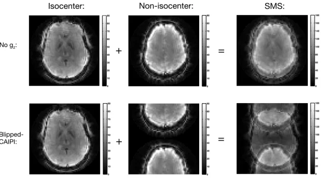
periodically go to 0 to minimize through-plane intravoxel dephasing. In other words, the z-gradient should contain rewinders to ensure that too much phase does not ac-cumulate along the z-direction. The method by Nunes et al. [39] did not use such rewinders, causing significant through-plane dephasing of the finite-thick slices. Set-sompop et al. [40] then developed the blipped-CAIPI method, which uses alternating gz(t) blips to overcome this issue.

The closely related methods by Nunes et al. and Setsompop et al. can be described by Figure 2.3, which gives a more intuitive explanation as to why the readout z -gradient modulation is beneficial for SMS imaging. Figure2.3 shows a 2 simultaneous slice acquisition with no readoutz-gradient in the top row, and a 2 simultaneous slice acquisition with a blipped z-gradient in the bottom row. The individual slices are shown in the left and center columns; the left column shows the slice that occurs atz -isocenter, and the middle column shows the slice that occurs some distance away. The

(33)

Non-Cartesian parallel SMS: Background

0 10 20 30 40 50 60 70 80 90 0 10 20 30 40 50 60 70 80 90 0 20 40 60 80 100 120 140 160 180 0 20 40 60 80 100 120 140 160 180 0 10 20 30 40 50 60 70 80 90 0 10 20 30 40 50 60 70 80 90 Isocenter: Non-isocenter: No gz: Blipped- CAIPI:

+

=

SMS:

Figure 2.3: Two simultaneous slice acquisitions with no readoutz-gradient (top row), and a blipped-CAIPI readoutz-gradient (bottom row). The SMS acquisition is shown in the right column, which is simply the sum of the individual slices shown in the left and middle columns.

resulting aliased simultaneous slice acquisition is shown in the right column. With noz-gradient, the simultaneously acquired slices are perfectly overlapped, making it difficult to separate them unless their sensitivities are very different. For blipped-CAIPI, the z-gradient shifts the non-isocenter slice, resulting in less overlap in the SMS acquisition. This results in easier slice separation.

The phases of the Mv matrices in Equation (2.19) differ from each other only by

the scalar multiplezv, so in order to make eachMv as different as possible to improve

conditioning, the simultaneous slices should be separated at even distances from each other. This way, the additional phase that each simultaneous slice experiences from the z-gradient modulation is spread out as much as possible in the z-direction. Fur-thermore, it is desirable to separate the simultaneous slices by the maximum distance possible in order to fully use the coil sensitivity information as part of the slice sepa-ration process; in general, slices further apart will have more differences in sensitivity

(34)

than slices that are nearby. An RF pulse that creates such a configuration can be written in the form of Equation (2.4), with ˜fv = fRF(v −1)∆z/ζ, where ∆z is the

distance between the simultaneous slices, and ζ is the slice thickness. An example slice profile for 3 simultaneous slices acquired in this manner is given in Figure 2.4. The full brain volume is covered by imaging consecutive slices with each successive

−4000 −2000 0 2000 4000 0 2 4 6 8 10 12 14 16 18 Frequency (Hz)

Figure 2.4: Slice profile for a 3 simultaneous slice acquisition created from the 6.4 ms Hamming-windowed sinc with 4 zero-crossings shown in Figure 2.1.

TR, while keeping the distance between the simultaneous slices the same. Using the previous expression for ˜fv with consecutive slices located right next to each other,

there would be ∆z/ζ acquisitions for a total of l∆z/ζ slices for the whole volume. However, one must be careful of phase wraps; if the magnitude of gz(t) is enough

to cause any number of phase wraps across thez-axis, the phase modulation for each simultaneous slice could end up being very similar even if the slices are all separated from each other by some even distance. For example, if z1, z2, and z3 are 0, 1, and

2, respectively, andγz3

Rt

0 gz(τ) dτ = 4π, then slice 2 experiences a phase modulation

(35)

1/3, and 2/3, respectively, then the modulation for slices 1, 2, and 3 are 0, 2π/3, and 4π/3, respectively, which is the maximum phase spread possible. From a Fourier perspective, this means that for simultaneous slices that are closer together, a higher kz value is needed, which means we need to use a larger gz(t) to go out further in

kz-space. This also means that for a given simultaneous slice separation distance,

a larger z-gradient is not necessarily better for reconstruction, even when ignoring through-plane dephasing effects.

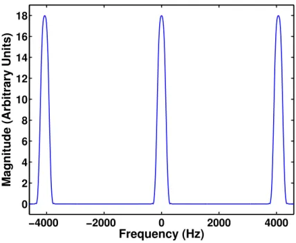
To better understand the effect of the readout z-gradient, Zahneisen et al. [41] introduced a general framework for SMS using a 3-dimensional Fourier viewpoint. They note that the simultaneous slices create a field of view (FOV) with accompanying resolution in the z-direction. The FOV is just

FOVz =l∆z, (2.21)

wherelis the number of simultaneously acquired slices and ∆z is the distance between simultaneous slices. Therefore, the necessary distance betweenk-space samples in the z-direction is ∆kz = 1 FOVz = 1 l∆z. (2.22)

The distance between simultaneous slices, ∆z, specifies the resolution δz in the z

-direction. The maximum extent of kz-space is then

k_zmax= 1 2δz = l 2FOVz = 1 2∆z = l∆kz 2 . (2.23)

(36)

Equation (2.19) for the xv vector. This problem is typically overdetermined since the

number of coils is greater than the number of simultaneous slices, and the number of k-space samples for each readout is comparable to the number of pixels in each slice for spiral imaging. In addition, noise from Eddy currents and hardware imperfections will be present in the raw data. Therefore, it can be beneficial to use the following regularized least squares problem for reconstruction:

ˆ

x= arg min x

kAx−sk2₂+βkRxk2₂ , (2.24)

whereA,x, andsare the system matrix,xv vector, andsu vector in Equation (2.19),

respectively. R is a finite differencing matrix, and β is the regularization parameter that controls the tradeoff between spatial resolution and noise reduction in the recon-struction ˆx. The least squares solution to (2.24) is ˆx= (A0A+βR0R)−1_A0_s_{, which}

can be computed using the Conjugate Gradient algorithm [42] and implemented using Jeffrey A. Fessler’s Image Reconstruction Toolbox [43].

Although x is 3-dimensional since it contains multiple 2-dimensional slices, R

cannot be a 3-dimensional finite differencing matrix because differences would be computed between pixels that are in different slices separated from each other by a relatively large distance. Since x consists of l separate slices, R should perform the operation of a block diagonal matrix with each block performing a 2-dimensional finite difference computation on a single slice. In other words, Rcan be implemented as R=          D1 0 0 0 0 D2 . .. 0 0 . .. ... 0 0 0 0 Dl          , (2.25)

(37)

construction ensures that differences are not computed between pixels that are in different slices.

The value ofβ can be chosen using resolution analysis of the system point spread function (PSF). The system PSF is defined as (A0A+βR0R)−1_A0_Ae

j, where ej is

thejth unit vector or “point.” After computing this value using Conjugate Gradient, the full-width-at-half-maximum (FWHM) of the PSF can be measured along each of the three physical dimensions of the image. In this dissertation, a FWHM in the slice plane of around 1.3 pixels was found to work well by inspection, which yielded a value of β = 273 for all the experiments.

In this dissertation, B0 inhomogeneity field maps are computed using an angle

measurement method [44] from two scans with different TEs: one with a TE of 30 ms, and one of 32 ms. First, the images themselves are reconstructed for each coil by effectively computing an inverse NUFFT of the k-space data for each coil using Conjugate Gradient. Then, the field map _∠(x0_w,u∗ x_w,u1 )/∆t is calculated, where x0_w,u is the wth pixel of coil u of one scan, x1_w,u is the wth pixel of coil u of the other scan, and ∆t is the difference in TEs between the two scans, which is 2 ms in this case. The field maps are then summed across coils and smoothed by convolving with a 7-by-7 constant kernel. Finally, the original 2 scans are reconstructed again with inhomogeneity correction using the new field map, and the process is repeated to obtain a better estimate of the field map.

Coil sensitivities can be obtained by directly computing

ˆ

cu,v = arg min

cu,v

kxu,v−Bvcu,vk₂2+λkDcu,vk2₂ , (2.26)

using ˆcu,v = (Bv0Bv+λD0D)−1Bv0xu,v, where cu,v is the sensitivity of coilu to slice

v, xu,v is the inhomogeneity-corrected reconstruction for coil u and slice v, Bv is a

(38)

and D is a 2-dimensional finite differencing matrix. Coil sensitivities can also be computed using more recent techniques such as ESPIRiT [45].

Note that the B0 inhomogeneity field maps and coil sensitivity maps must be

computed from a non-SMS acquisition that has at least the same number of slices per volume as the reconstructed SMS scan, and with individual slices at the same locations as those for the SMS scan. For all the SENSE experiments in this dissertation, a separate non-SMS acquisition with matching slice locations was performed before each SMS scan.

Along with blipped-CAIPI, Setsompop et al. [40] also developed slice-GRAPPA, a k-space reconstruction scheme for slice separation. Slice-GRAPPA uses a different convolution kernel to construct thek-space data for each coil of each separated slice. Figure 2.5 illustrates the kernel operation for one coil of one separated slice. Each

Non-Cartesian parallel SMS: Background

coils SMS k-space

k-space of 1 coil of

separated slice

Figure 2.5: Slice-GRAPPA kernel operation to compute thek-space data for one coil of one separated slice. Each kernel operates on all coils of the SMS k-space data.

(39)

kernel operates on all coils of the SMS k-space data. A different kernel is needed to compute a different coil of that same slice in Figure 2.5. Finally, a whole set of additional kernels are needed to compute all the coils of another separated slice.

Moeller et al. [46] demonstrated the use of Cartesian SMS imaging in fMRI at 7 T, but did not use a CAIPI approach to improve theg-factor. Their demonstration used coronal slices to improve the g-factor because this orientation, along with a sagittal orientation, provided the most differences in coil sensitivity from slice to slice. They used the SENSE/GRAPPA [47] reconstruction method to separate the slices.

Recently, Zahneisen et al. [48] adapted blipped-CAIPI to single-shot spirals and demonstrated SMS imaging with a blipped spiral-in readout. An example of a blipped spiral trajectory for a 3 simultaneous slice acquisition is shown in Figure2.6. In fMRI, spiral-in readouts have advantages over Cartesian-based ones like echo planar imaging (EPI) such as better signal recovery [49] and shorter readout times [17, 50], which reduces off-resonance distortion and also increases the maximum number of slices acquired per unit time. Furthermore, spiral trajectories have reduced sensitivity to motion when compared with EPI [51].

(40)

−200 −100 0 100 200 −200 −100 0 100 200 −10 −5 0 5 10

k

y

(cycles/m)

k

x

(cycles/m)

k

z

(cycles/m)

Figure 2.6: Three-dimensional blipped spiralk-space trajectory for a 3 simultaneous slice acquisition.

(41)

CHAPTER 3 Hadamard-encoded Simultaneous

Multislice fMRI

1

3.1 Hadamard-encoding

for

Reduced

Signal

Dropout

Hadamard-encoded SMS can be used to acquire thinner slices in order to reduce the signal dropout from through-plane dephasing. In Ref. [30], a method involving an incoherent addition of subslices, described by Equation (2.14), was proposed. In this section, it is shown that there is a signal recovery benefit to reconstructing the individual subslices first, then combining them afterwards. Similar to what was done in Ref. [30], two simultaneous subslices are acquired with each acquisition in this section. The conventional non-SMS comparison has individually acquired slices, each with width equal to the combined width of two simultaneous Hadamard-encoded subslices. In other words, the width of each Hadamard subslice is one-half that of a conventional slice.

3.1.1 Separation of Slices for Reduced Signal Dropout

In Ref. [30], Hadamard-encoded SMS images were reconstructed by filtering the squared magnitude of the signal as described by Equation (2.14), which results in

(42)

the magnitude combination of subslices given by Equation (2.15). However, this is not an optimal slice combination in terms of reducing signal dropout.

For example, assume that a conventional acquisition is performed with no susceptibility-induced field gradients. Substituting ∆θ = 0 in Equation (2.11), we have |I_nconv|= q S2 1,n+S22,n+ 2S1,nS2,nθ = q (S1,n+S2,n)2 =S1,n+S2,n,

which is just the sum of the magnitudes of each subslice. However, with the recon-struction of Hadamard-encoded SMS proposed by Ref. [30], the resulting data has magnitudeqS2

1,n+S22,n, as given by Equation (2.15). This is equivalent to the signal

obtained with a conventional acquisition where there is a ∆θ =π/2 phase difference between subslices, seen by substituting ∆θ = π/2 in Equation (2.11). In fact, since 0 < cos ∆θ < 1 for −π/2 < ∆θ < π/2, a conventional acquisition has better sig-nal recovery compared to a Hadamard acquisition when the phase difference between subslices is less thanπ/2. Only when the phase difference between subslices is greater thanπ/2 does Hadamard-encoded SMS have better signal recovery using the method proposed by Ref. [30].

For the purposes of reduced signal dropout, it is better to reconstruct the individ-ual Hadamard-encoded subslices, then combine the subslices. In other words, filter the complex Hadamard-encoded signal IHada

n given by Equation (2.12) to obtain

S1,neiφ =F−1{WnF(InHada)}, (3.1)

(43)

the complex time series, then low-pass filter to obtain

S2,nei(φ+∆θ)=F−1{WnF(i(−1)n+1InHada)}. (3.2)

For sufficiently large S1,n and S2,n, ∆θ can be estimated by taking the difference of

the phases of S1,neiφ and S2,nei(φ+∆θ), then S1,neiφ and S2,neiφ can be summed and

transformed into the object domain. Alternatively, if the global phaseφis not needed, the magnitudes S1,n and S2,n can be simply summed and transformed. In this case,

the magnitude of the signal will beS1,n+S2,nregardless of the value of ∆θ, equivalent

to a conventional acquisition with no susceptibility-induced field gradients.

3.1.2 SNR Analysis

Ref. [30] also makes the claim that using a low-pass filter Wn with cutoff one-half

the Nyquist frequency, their proposed Hadamard-encoding has an SNR advantage over conventional acquisitions. Assuming equal magnitudes of 1 in each subslice and uncorrelated thermal noise with standard deviation σ0 in each acquisition, the SNR

for a conventional acquisition due to thermal noise is

SNRconv₀ =

√

2 + 2 cos ∆θ σ0

, (3.3)

since the signal magnitude given by substitutingS1,n =S2,n = 1 into Equation (2.11)

is justSconv ₌√_{2 + 2 cos ∆}_θ_.

For their proposed Hadamard-encoded SMS, the signal magnitude from Equa-tion (2.15) is SHada ₌√₁2 _{+ 1}2 ₌ √_{2, assuming that the low-pass filter}_W

n behaves

perfectly. To compute the effects of the low-pass filter Wn, they use Parseval’s

the-orem, which states that the variance of the signal is reduced by the area under Wn.

In other words, σ₀2 is reduced to cσ₀2, where c = _N1 PN−1

n=0 W 2

(44)

Therefore, the SNR for a Hadamard-encoded acquisition due to thermal noise is SNRHada₀ = √ 2 σ0 √ c. (3.4)

Rewriting Equation (3.4), we have

SNRHada₀ = 1 √ c √ 2 √ 2 + 2 cos ∆θ ! √ 2 + 2 cos ∆θ σ0 = √ 2 √ c√2 + 2 cos ∆θ ! √ 2 + 2 cos ∆θ σ0 = _p 1 c(1 + cos ∆θ) ! SNRconv₀ . (3.5)

Assuming no susceptibility-induced field gradients so that ∆θ= 0, when the low-pass filter cutoff is half the Nyquist frequency, then c = 1₂, making SNRHada₀ = SNRconv₀ . With no filtering, c = 1 so that Equation (3.5) becomes SNRHada₀ = √1

2

SNRconv₀ , which makes sense since with no through-plane dephasing, Sconv = 2 and SHada = Sconv/√2, so SNRHada₀ =SHada/σ0 =Sconv/(σ0

√ 2) = 1 √ 2 SNRconv₀ .

From Ref. [54], the SNR of a signal S with total image noise standard deviation σ is SNR = S σ = _q S σ2 0+σp2 = _p S σ2₀+λ2_S2, = S σ0 p 1 +λ2_S2_/σ2 0 , = _p SNR0 1 + (λSNR0)2 , (3.6) whereσ2 ₌_σ2

0+σ2p,σp2 is the variance from physiological noise, andσp =λS, whereλ

Simultaneous Multislice Functional Magnetic Resonance Imaging.