ISSN: 2319-5967
ISO 9001:2008 Certified
International Journal of Engineering Science and Innovative Technology (IJESIT) Volume 3, Issue 5, September 2014
335
A Mathematical Model of the fluid flow in
Circular Cross-sectional Open Channels
V.N. Ojiambo, M. N. Kinyanjui, D. M. Theuri, P. R. Kiogora, K. Giterere
Abstract: Open channel flow involves the flow of a fluid in a channel or conduit that is not completely filled. This
study examines a non-uniform and unsteady open channel flow with circular cross-sectional area that runs partly filled. The flow variables are velocity and depth while the flow parameters are cross-sectional area of the channel, channel radius, slope of the channel and lateral inflow rate per unit length of the channel. Effects of cross sectional area of the channel on the flow velocity, the effects of channel radius, slope of the channel and lateral inflow rate per unit length of the channel on the flow velocity are investigated. This is done by varying one parameter while holding the other parameters constant. The study further investigates the maximum flow depth. The momentum and the continuity equations are the governing equations of this flow. The momentum equation is expanded using the unsteady state of the continuity equation. Finite difference approximation method has been used to solve the governing equations due to its accuracy, stability and convergence characteristics. The results have been graphically presented. It is established that increase in the cross-sectional area leads to decrease in the flow velocity, an increase in the radius of the channel leads to decrease in the flow velocity, an increase in the roughness coefficient leads to decrease in the flow velocity, an increase in the flow depth leads to decrease in the flow velocity and a decrease in the lateral inflow rate per unit length of the channel leads to an increase in the flow velocity.Index terms:
Open channel, velocity, depth.I. INTRODUCTION
Many researchers have ventured to study open channel flows but few concentrated on the circular channel flows because of their difficulty in construction. Circular channel flows increase the flow velocity due to the minimum wetted perimeter that they have. Chow [1] studied Open Channel flows and developed many relationships such as velocity formula for open channel flow. He is also one of the pioneers in the definition of the geometric elements of an open channel flow. The prediction of the one-dimensional flow characteristics (e.g. free surface profile and local distribution of discharge) is based upon the dynamical flow equation. Application of the longitudinal momentum theorem yields a generalized backwater relation as extended by Yen and Wenzel [2]. The dynamical flow equation must be completed by the lateral outflow law and expressions relating to the momentum correction coefficient, the lateral outflow velocity component in the longitudinal direction and the friction slope. The usual approach assumes a uniform velocity distribution, and is based on the energy equation, in which losses are accounted for by Manning's formula. Strelkoff [3] and Yen [4] derived the energy equation from integration of Navier stokes equations. They clearly demonstrated that the losses of the mechanical energy are due to the work done by the internal stresses to overcome velocity gradient. Sinha et al. [5] investigated the development of the laminar flow of a viscous incompressible fluid from the entry of a straight circular pipe. It was observed that the velocity increases more rapidly during the initial development of the flow in comparison to the downstream flow. It was observed that during the initial stages of the development of the flow, the rate of increase in stream wise velocity is larger and consequently the pressure drop is larger in comparison with their values further downstream. This is because the retarded fluid particles in the boundary layer are pushed towards the core more rapidly near the entry where the boundary layer is thinner as compared to the downstream region. The influence of lateral mass flux on free convection flow past a vertical flat plate embedded in a saturated porous medium was studied by Mansour et al. [6].Hager [7] studied the lateral outflow mechanism of side weirs using a one-dimensional approach. In particular, the effects of flow depth, approaching velocity, lateral outflow direction and side weir channel shape were included, resulting in expressions for the lateral outflow angle and the lateral discharge intensity. For vanishing channel velocity, the conventional weir formula for plane flow conditions was reproduced. However, for increasing local Froude number, the lateral outflow intensity decreases under otherwise fixed flow parameters. A comparison of the theoretically determined solution with observations indicated a fair agreement. The results were then applied to open channel bifurcations by considering a side-weir of zero weir height. Distinction between sub- and supercritical flow conditions is made. Again, the computed
ISSN: 2319-5967
ISO 9001:2008 Certified
International Journal of Engineering Science and Innovative Technology (IJESIT) Volume 3, Issue 5, September 2014
336
results compare well with the observations and allow a simple prediction of all pertinent flow characteristics. Crossley [8] investigated the strategies developed for the Euler’s equations for application to the Saint Venant equations of open channel flow in order to reduce run times and improve the quality of solutions in the regions discontinuities. Nalluri et al. [9] analyzed experimental date on resistance to flow in smooth channels of circular cross section. The results of the tests showed that the measured friction factors are larger than those for a pipe of equivalent diameter
(D
-
4R).
Through the analysis of the data for the range of flow depths0
<
y
<
0.85d,
the geometric parameter y/P was found more appropriately representing the shape effects on resistance to flow in circular channels than using a single parameter like the hydraulic mean radius, R. Carlos and Santos [10] considered an adjoint formulation for the non-linear potential flow equation. Tuitoek and Hicks [11] modeled unsteady flow in compound channels with an aim of controlling floods. Kwanza et al. [12] analyzed the effects of the channel width, slope of the channel and lateral discharge on fluid velocity and channel discharge for both rectangular and trapezoidal channels. They noted that the discharge increases as the specified parameters are varied upwards. Ayhan [13] set up A Neutralized Based Fuzzy Reference System (ANFIS) for prediction of friction coefficient in open channel flows in which Reynold’s number velocity and discharge are used as inputs to determine friction coefficient of an open channel flow. It was shown that when provided with correct and sufficient samples, ANFIS model can be used to predict the non-linear relationship between friction coefficient and the factors which affect it. It was concluded that, in practice, ANFIS model can be used as a suitable and effective method and general hydraulic problems which are mostly based on laboratory tests can be analyzed with ANFIS model. M.N. Kinyanjui et al. [14] investigated on modeling fluid flow in open channel with circular cross-section. This study considered unsteady non-uniform open channel flow in a closed conduit with circular cross-section. The main objectives were to investigate the effects of the flow depth, the cross section area of flow, channel radius, slope of the channel, roughness coefficient and energy coefficient on the flow velocity as well as the depth at which flow velocity is maximum. The obtained Saint-Venant partial differential equations of continuity and momentum governing free surface flow in open channels are nonlinear and therefore do not have analytical solutions. The Finite Difference Approximation method is used to solve these equations because of its accuracy, stability and convergence. Patel [15] described a hydraulic model, testing of various important structures of open channel as well as river flow with analytical solution of the flow distribution along the open channel. The study considered different roughness constant and different flow rate to examine the flow pattern in an open channel. The research enabled the prediction of the velocity profile of open channel flow that would be applicable for a wide range of Reynolds number by changing the discharge flow rate.
II. MATHEMATICAL ANALYSIS
Governing equations
The Continuity and the Momentum or the energy equations may be used to analyze open channel flow. Except for the momentum coefficient
and the energy coefficient
, the Momentum and energy equations are equivalent; Cunge et al. [16] provided that the flow depth and velocity are continuous i.e. there are no discontinuities along the channel flow. However the Momentum should be used if there are no discontinuities, since, unlike the energy equation it is not necessary to know the amount of losses in the discontinuities in the application of momentum equation. This study considers the Continuity and Momentum equations with velocity and flow depth as the two flow variables. The statement of the problem is a circular conduit that runs partly filled at certain times. The governing equations discussed herein are borrowed from conservation of mass and momentum principle given by Yen [4];The cross-sectional area A is taken from the volume element shown below where the displacement is in the main flow direction(x) given by , where the flow fluid enters from volume element at section U at a mass transfer rate of and leaves at section D at a mass transfer rate of .
ISSN: 2319-5967
ISO 9001:2008 Certified
International Journal of Engineering Science and Innovative Technology (IJESIT) Volume 3, Issue 5, September 2014
337
In this study the flow is unsteady and non-uniform. From M.N. Kinyanjui et al. [14], the continuity equation is given by
q
t
A
x
Q
(1) which is expanded to0
T
q
x
V
T
A
x
y
V
t
y
(2)The momentum equation is given by Yen 1973 [4];
0
0
fS
S
gA
x
y
gA
QV
x
t
Q
(3)The cross-sectional area of this study is a uniform circular cross-section, thus the value of momentum coefficient is equal to one. Replacing the continuity equation for unsteady flow the momentum equation becomes:
0
0
g
S
S
fx
y
g
x
V
V
t
V
A
Vq
(4)The solution procedure
The governing equations; equation (2) and (4), are solved using a diffusing finite difference scheme as proposed by Viessman et al.[17].These equations are given as:
T
q
h
V
V
T
A
h
y
y
V
k
y
y
y
i j i j i j i j i j i j i j i j2
2
5
.
0
1, 1 1, , 1, 1, 1, 1, 1 , (5)
j i j i j i j i j i j i j i j i j i j i j iV
V
R
n
S
g
h
y
y
g
h
V
V
V
k
V
V
V
A
q
V
, 1 2 , 1 2 3 4 2 0 , 1 , 1 , 1 , 1 , , 1 , 1 , 1 ,2
2
2
5
.
0
(6)subject to the initial conditions
V(0,
t)
=
20,
y(x,0)
=
4.5
for
all
x
>
0
and boundary conditions Fig 1: Volume elementISSN: 2319-5967
ISO 9001:2008 Certified
International Journal of Engineering Science and Innovative Technology (IJESIT) Volume 3, Issue 5, September 2014
338
0.
>
t
all
for
4.5
=
y(x,0)
20,
=
t)
V(0,
III. RESULTS AND DISCUSSION
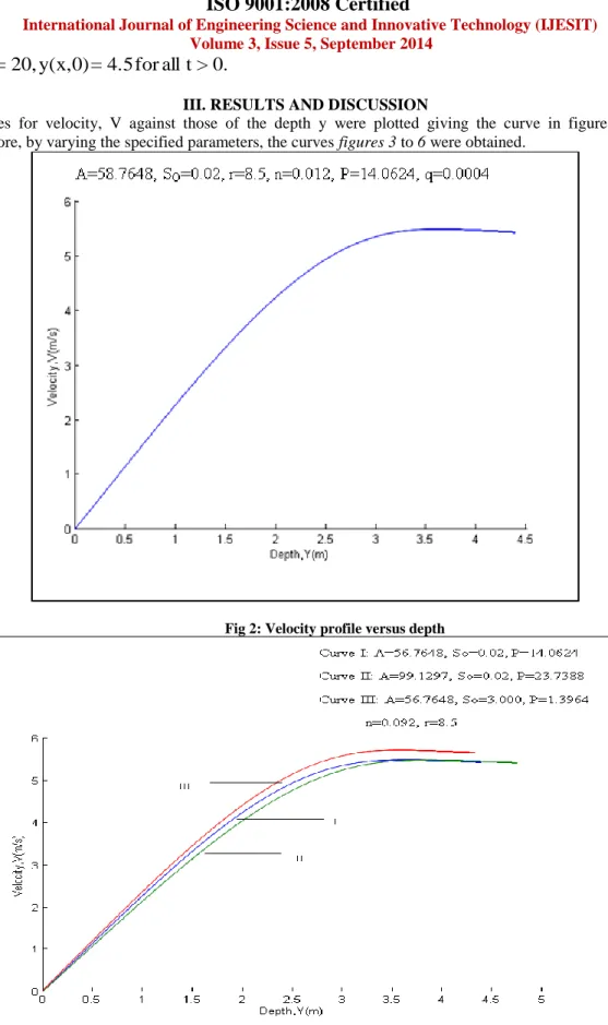
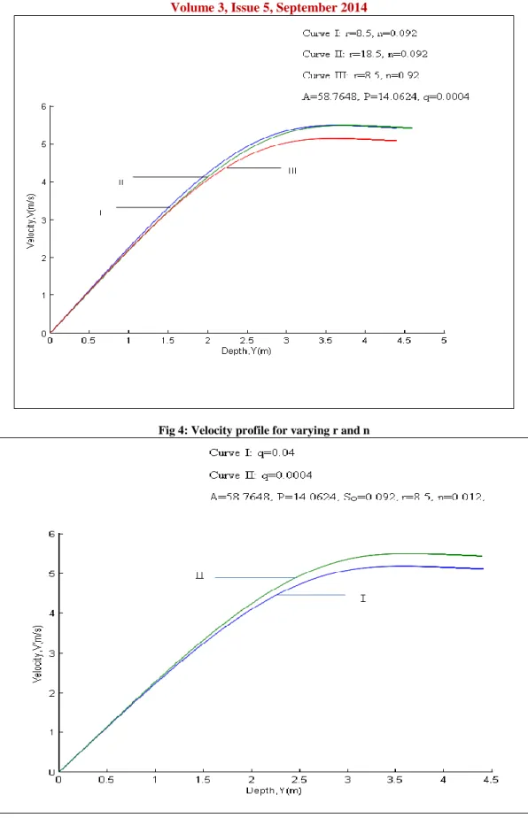
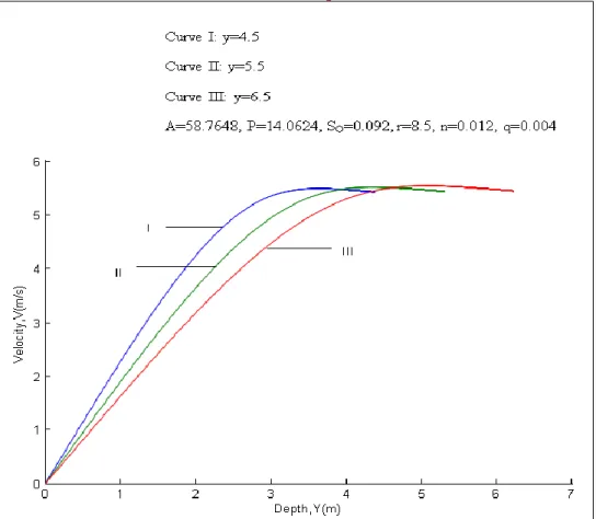
The values for velocity, V against those of the depth y were plotted giving the curve in figure 2 below. Furthermore, by varying the specified parameters, the curves figures 3 to 6 were obtained.
Fig 2: Velocity profile versus depth
ISSN: 2319-5967
ISO 9001:2008 Certified
International Journal of Engineering Science and Innovative Technology (IJESIT) Volume 3, Issue 5, September 2014
339
Fig 4: Velocity profile for varying r and n
ISSN: 2319-5967
ISO 9001:2008 Certified
International Journal of Engineering Science and Innovative Technology (IJESIT) Volume 3, Issue 5, September 2014
340
Fig 6: Velocity profiles for varying depth
Figure 2 shows that velocity increases with increase in depth. The free surface occurs at a depth of 4.5m and the velocity of the fluid at this depth is 10m/s. It is also observed that the maximum velocity occurs at a depth of 3.5m and begins to decrease in velocity as it approaches the free surface.
The flow velocity in a channel varies from one point to another as a result of shear stress at the bottom and the sides of the channel. The free surface does not exhibit maximum velocity due to surface tension caused by strong cohesive forces among the liquid molecules. Each liquid molecule is pulled equally in every direction by neighboring liquid molecules resulting into a conservative net force. At the free surface occurs a gaseous-liquid interface whereby the liquid molecules are attracted inwards to other liquid molecules rather than outward to the gaseous molecules. This creates internal pressure among the liquid molecules that forces the liquid surface to contract leading to a reduction in velocity at the free stream. Millions of collisions take place between the atmosphere and liquid molecules. As a result, the atmospheric pressure exerts some surface force on the water surface and gravity creates internal pressure that causes contraction of the liquid surface resulting to reduced velocities. Furthermore, the wind blowing over the free surface also affects the velocity due to frictional resistance particularly when wind blows over the free surface at high velocities and in the opposite direction to the main flow direction.
Figure 3 shows that increase in the slope from 0.02 to 3.000 leads to increase in the flow velocity i.e. from Curve I to Curve III. It also shows that increase in the cross-sectional area from 56.7648 to 99.1297 leads to decrease in the flow velocity i.e. Curve I to Curve II. Increase in the slope causes the center of gravity to move up causing instability in the water molecules. The direct relationship of the flow is show in equation 2.11 where an increase in slope causes an increase in the flow velocity. Increase in the cross-sectional area of flow leads to increase in the wetted perimeter that leads to increase in the shear stress between the sides and bottom of the channel with the fluid particles which results to decrease in the flow velocity.
ISSN: 2319-5967
ISO 9001:2008 Certified
International Journal of Engineering Science and Innovative Technology (IJESIT) Volume 3, Issue 5, September 2014
341
Figure 4 shows that an increase in the radius of the channel from 8.5m to 18.5m leads to a decrease in the flow velocity i.e. from Curve I and Curve II. It also shows that an increase in the roughness coefficient from 0.092 to 0.92 leads to a decrease in the flow velocity. An increase in the radius of the channel results to an increase in the wetted perimeter as a result of the fluid spreading more in the conduit leading to a larger cross-sectional area. A large wetted perimeter results to large shear stresses at the sides and bottom of the channel leading to reduction in velocity. An increase in the roughness coefficient results to large shear stress at the sides of the channel. This means that the motion of the fluid particles at or near the surface of the conduit will be reduced. The velocity of the neighboring molecules will also be lowered due to constant bombardment with the flow moving molecules leading to an overall reduction to the flow velocity.
Figure 5 shows that a decrease in the lateral inflow rate per unit length of the channel from 0.04 to 0.004 leads to an increase in the channel velocity i.e. from Curve I to Curve II. An increase in the lateral inflow rate per unit length of the channel means an increase in the amount of flow per unit time. This leads to increase in the cross-sectional area of which leads to increase in the wetted perimeter that increases the shear stress between the sides and bottom of the channel with the fluid particles leading to decrease in the flow velocity.
Figure 6 shows that an increase in the channel depth from 4.5m to 5.5m to 6.5m i.e. Curve I to Curve II to Curve III leads to a decrease in the channel velocity. An increase in the flow depth leads to increase in the wetted perimeter which results to increase in the shear stresses at the sides of the channel that results to decrease in the flow velocity.
IV. CONCLUSION
A circular channel flow has been developed with the resulting partial differential equations solved to obtain the velocity profiles using the velocity and depth as the flow variables. There is a reasonable agreement between the results of our model and those published by different authors. This proves the fidelity of our equations and the numerical scheme used.
ACKNOWLEDGEMENT
The authors gratefully acknowledge the support of Pure and Applied Mathematics department of Jomo Kenyatta University of Agriculture and Technology, Mr. P.R. Kiogora and Dr. Kang’ethe for their technical assistance.
NOMENCLATURE A: Cross-sectional area (m2)
P: Wetted Perimeter (m)
: Manning roughness coefficient (sm-1/3)
Q: Discharge (m3s-1)
T: Top width
: Lateral inflow rate per unit length of the channel (m2s-1)
R: Hydraulic radius (m)
Sf: Frictional slope
So: Longitudinal slope of the channel
: Time(s)
V: Velocity of flow
ISSN: 2319-5967
ISO 9001:2008 Certified
International Journal of Engineering Science and Innovative Technology (IJESIT) Volume 3, Issue 5, September 2014
342
: Main flow direction
: Momentum coefficient α: Energy coefficientREFERENCES
[1] Chow V. T. Open Channel hydraulics. McGraw Hill Book Company. New York: pp1-40, (1959).
[2] Yen, B. C, and Wenzel, H. G. "Dynamic Equations for Steady Spatially Varied Flow," Journal of the Hydraulics Division, ASCE, Vol.96, No. 3, pp801-814, (1970).
[3] Strelkoff, T., “One-dimensional equations of open-channel flow,” Journal of the Hydraulics Division, ASCE, Vol. 95(HY3), pp 861–876, (1969).
[4] Yen, B. C. ,“Open-channel flow equations revisited,” Journal of the Engineering Mechanics Division, ASCE, Vol. 99(EM5), pp 979–1009, (1973).
[5] Sinha, P.C. and Meena Aggarwal, Entry flow in a straight circular pipe, Journal of Australian Mathematics (Series BG), pp59-66, (1982).
[6] Mansour, M.A., Hassanien, J.A AND Bakier, A, Y., The influence of lateral mass flux on free convection flow past a vertical flat plate embedded in a saturated porous medium, Indian Journal of Pure Appl. Math., Vol. 21(3), pp 238-245, (1990).
[7] Hager, VV. H., and Volkert, P. U. , "Distribution Channels," Journal of Hydraulic Engineering, ASCE,Vol.112, No. 10 pp 935-952, (1986).
[8] Crossley Amanda Jane, Accurate and efficient numerical solutions for the Saint Venant equations of open channel flow, Ph.D thesis, University of Nottingham, United Kingdom, (1999).
[9] Nalluri C. and Adepoju B.A., Shape effects on resistance to flow in smooth channels of circular cross section. Journal of Hydraulic Research, Vol. 23. Issue 1 January, pp 37-46, (1985).
[10]Carlos L. and Santos C., An adjoint for the non-linear potential flow equation, Appl. Math. Comp.Vol. 108, pp11-12, (2000).
[11]Tuitoek, D.K. and Hicks, F.E., Modeling of unsteady flow in compound channels, African Journal Civil Engineering Vol.4, pp. 45-53, (2001).
[12]Kwanza, J.K.,Kinyanjui M. and Nkoroi, J.M., Modeling fluid flow in rectangular and trapezoidal open channels. Advances and Applications in Fluid Mechanics, Vol.2, pp. 149-158, (2007).
[13]Ayhan Samandar,”A Neutralized Based Fuzzy Reference System (ANFIS) for prediction of friction coefficient in open channel flows” , Academic journals , Scientific Research and Essays Vol.6(5), pp 1020-1027, (2010).
[14]MM Kinyanjui, DP Tsombe, JK Kwanza, K Giterere, Modeling Fluid Flow in Open Channel with Circular Cross-section, Journal of Agriculture, Science and Technology Vol.13, No. 2, (2011).
[15]Kaushal Patel, “Mathematical model of open channel flow for estimating velocity distribution through different surface roughness and discharge”, International Journal of Advanced Engineering Technology, IJAET, Vol. III, Issue I, January-March, pp 252-253, (2012),
[16]Cunje, J. A. Holly, F.M. Jr and Verwey, A., “Practical aspects of river computational hydraulics”, Pitman London. (1980).
[17]Viessman W, Jr. Knapp J.W., Lewis G. L., and Harbaugh T.E., “Introduction to hydrology”, Second edition, Harper and Row, New York, pp. 1-60, (1972).
ISSN: 2319-5967
ISO 9001:2008 Certified
International Journal of Engineering Science and Innovative Technology (IJESIT) Volume 3, Issue 5, September 2014
343
AUTHOR BIOGRAPHY
Miss. Viona Nakhulo Ojiambo obtained her BSc. in Applied Mathematics and Computer Science from Jomo Kenyatta University of Agriculture and Technology (JKUAT), Kenya in 2011. Presently she is working as an Adjunct Teaching Assistant at JKUAT. She is a MSc. student in the same university. Her area of research is Channel Flows.
Professor Mathew Ngugi Kinyanjui Obtained his MSc. In Applied Mathematics from Kenyatta University, Kenya in 1989 and a PhD in Applied Mathematics from Jomo Kenyatta University of Agriculture and Technology (JKUAT), Kenya in 1998. Presently he is working as a professor of Mathematics at JKUAT where is also the director of |Post Graduate Studies. He has Published over Fifty papers in international Journals. He has also guided many students in Masters and PhD
courses. His Research area is in MHD and Fluid Dynamics.
Dr. David Mwangi Theuri Obtained his MSc. In Applied Mathematics from Kenyatta University, Kenya in 1990 and a PhD in Applied Mathematics from Jomo Kenyatta University of Agriculture and Technology (JKUAT), Kenya in 2001. Presently he the Chairperson of the Department of Pure and Applied Mathematics at JKUAT. He has Published over ten papers in international Journals. He has also guided many students in Masters and PhD courses. His Research area is in MHD and Fluid Dynamics.
Mr. Phineas Roy Kiogora obtained his MSc. in Applied Mathematics from Jomo Kenyatta University of Agriculture and Technology (JKUAT), Kenya in 2007. Presently he is working as an Assistant Lecturer at JKUAT. He is a PhD student in the same university. His area of research is Hydrodynamic Lubrication.
Dr. Kang’ethe Giterere obtained his MSc. In Applied Mathematics from Jomo Kenyatta University of Agriculture and Technology (JKUAT), Kenya in 2007 and a PhD in Applied Mathematics from the same university in 2012. Presently he is working as a Lecturer at JKUAT. He has published six papers in international journals and guided many students in Masters courses. His area of research is MHD and Fluid Dynamics.