Pipeline Risk Assessment Using Dynamic Bayesian Network (DBN) for Internal Corrosion

(1)

PIPELINE RISK ASSESSMENT USING DYNAMIC BAYESIAN NETWORK (DBN) FOR INTERNAL CORROSION

A Thesis by

VISALATCHI PALANIAPPAN

Submitted to the Office of Graduate Studies of Texas A&M University

in partial fulfillment of the requirements for the degree of

MASTER OF SCIENCE

Chair of Committee, M. Sam Mannan Committee Members, Jerome Schubert Debjyoti Banerjee Head of Department, M.Nazmul Karim

August 2018

Major Subject: Safety Engineering

(2)

ii

ABSTRACT

Pipelines are the most efficient mode of transportation for various chemicals and are considered as safe, yet pipeline incidents remain occurring. Corrosion is one of the main reasons for incidents especially in subsea pipelines due to the harsh corrosive environment that prevails. Corrosion can be attributed to 36% amongst all the causes of subsea pipeline failure. Internal corrosion being an incoherent process, one can never forecast exact occurrences inside a pipeline resulting in highly unpredictable risk. Therefore, this paper focuses on risk assessment of internal corrosion in subsea pipelines. Corrosion is time-dependent phenomena, and conventional risk assessment tools have limited capabilities of quantifying risk in terms of time dependency.

Hence, this paper presents a Dynamic Bayesian Network (DBN) model to assess and manage the risk of internal corrosion in subsea. DBN possesses certain advantages such as representation of temporal dependence between variable, ability to handle missing data, ability to deal with continuous data, time- based risk update, observation of the change of variables with time and better representation of cause and effect relationship. This model aims to find the cause of internal corrosion and predict the consequence in case of pipeline failure given the reliability of safety barrier in place at each time step. It also demonstrates the variation of corrosion promoting agents, corrosion rate and safety barriers with time.

(3)

iii

DEDICATION

My parents,

RM. Palaniappan Kannan & Ponni Palaniappan My husband,

Thenappan Narayanan All my friends

(4)

iv

ACKNOWLEDGEMENTS

I would like to extend my genuine appreciation and deepest gratitude to the following persons without whom completing this study would have been impossible.

My graduate advisor, Dr. M. Sam Mannan for giving me an opportunity to pursue my MS in Safety Engineering at such a prestigious university. I am grateful to his supervision, inspiration and advice. My committee members, Dr. Debjyoti Bannerjee and Dr. Jerome Schubert for giving their valuable comments and suggestion. Research professor, Dr. Hans Pasman for his time, effort and patience in guiding me throughout to complete this study. My father, Mr. Palaniappan Kannan for his consistent help, encouragement and support. And finally, all the members of MKOPSC and support staffs for helping me and making sure that I am headed towards the right direction.

(5)

v

CONTRIBUTORS AND FUNDING SOURCES

Contributors

This work was supported by a thesis committee consisting of my graduate advisor, Dr. Sam Mannan, visiting research professor of MKOPSC, Dr. Hans Pasman, Committee members Dr. Debjyoti Banerjee of the department of mechanical engineering and Dr. Jerome Schubert of the department of petroleum department.

Funding sources

There are no outside funding contributions to acknowledge related to the research and compilation of this document.

(6)

vi

NOMENCLATURE

σg Standard deviation of limit state function

μg Mean of limit state function

σf Flow stress of pipe

σu Ultimate tensile strength

λDU Dangerous failure rate dangerous undetected

Δt Time Interval

A Actuator

AHP Analytical Hierarchy Process

C1 Consequence that there is no loss of containment C2 Consequence that there is limited loss of containment C3 Consequence that there is huge loss of containment CPT Conditional Probability Table

CR Corrosion Rate

D Diameter of pipe

DAG Directed Acyclic Graph

DBN Dynamic Bayesian Network

d(t) Defect depth

do Initial defect depth

ESD Emergency Shutdown

ETA Event Tree Analysis

FTA Fault Tree Analysis

(7)

vii

L Load

l Defect length

LS Logic Solver

LSF/g Limit State Function

M Folias factor

MCS Monte-Carlo Simulation

MFS Mass Flow Sensor

OODBN Object-oriented Dynamic Bayesian Network

P Internal pressure

PFD Probability of failure of demand POF Probability of failure of the pipeline Pll Probability of large leak

Prp Probability of rupture

PS Pressure Sensor

Psl Probability of small leak

R Resistance

rbp Maximum pressure the pipe can withstand before it could

collapse

rrp Maximum pressure the pipe can withstand before it

could rupture

t Time

TI Test time interval

(8)

viii

LIST OF FIGURES

Figure 1: Elements for corrosion mechanism ... 11

Figure 2:Representation of FT ... 13

Figure 3: Example of BN ... 15

Figure 4:Mapping algorithm of FT to BN (Khakzad, 2011) ... 17

Figure 5:Quantitative mapping of FT to BN (Barua, 2012) ... 18

Figure 6:Example of DBN ... 19

Figure 7:Framework for the pipeline internal corrosion model based on Dynamic Bayesian ... 21

Figure 8:Temporal dependence of corrosion promoting variables between adjacent time steps . 22 Figure 9:Temporal dependence of corrosion rate between adjacent time steps ... 23

Figure 10: Conversion of normal distribution to standard normal distribution (Arora, 2011) ... 26

Figure 11: Calculation of POF of pipeline ... 27

Figure 12: ETA of pipeline failure ... 29

Figure 13: OODBN of subsea pipeline internal corrosion risk assessment ... 31

Figure 14: FT of internal corrosion in the subsea pipeline(Khan,2016) ... 35

Figure 15: Framework of static BN ... 37

Figure 16: Framework of DBN for internal corrosion occurrence ... 38

Figure 17: Representation of interdependencies between equation nodes for corrosion rate calculation ... 39

Figure 18: BN framework representing the calculation of probability of failure of pipeline ... 42

Figure 19: Probability of LSF1 being less than 0 ... 43

Figure 20: Probability of LSF2 being less than 0 ... 43

(11)

xi

Figure 22: POF of pipeline ... 44 Figure 23: Workflow of components in ESD system ... 46

(12)

xii

LIST OF TABLES

Table 1 PFD calculation for voting architecture ... 28

Table 2 Definition of different consequences ... 29

Table 3 Pipeline parameters used in case study ... 33

Table 4 Probability of primary events in FT ... 36

Table 5 Conditional probability table of other corrosion promoting agent at ‘t+2’ ... 38

Table 6 Conditional probability table of H2O agents at ‘t+2’ ... 38

Table 7 Conditional probability table of CO₂ at ‘t+2’... 38

Table 8 Posterior probabilities for corrosion promoting agents at time ‘t’ ... 40

Table 9 Posterior probabilities for corrosion promoting agents for all the time steps except at time ‘t’ ... 41

Table 10 Estimation of PFD of ESD system ... 47

(13)

1

CHAPTER I

INTRODUCTION

Pipelines are the lifeline of oil/gas and petrochemical industries. They are efficient, reliable, safer, environmentally friendly and economical (Bharadwaj, 2014); yet; pipeline incidents remain a petrifying factor exposing industries to scrutiny.

Hence, pipeline industries have an obligation to identify hazards and deal with risks invariably throughout the lifetime of the pipeline to avoid incidents and economic loss as much as possible. Therefore, to meet their obligation, a risk assessment tool is recommended to help explain pipeline failure and its consequences, analyze risk and take decision for mitigation and prevention of risk more effectively, make the calculations and analysis less tedious and produce robust results. There had been 1,978 incidents between the years 2001 and 2011 in UK continental shelf according to UK health and safety executive, 2011, due to offshore hydrocarbon release. According to PHMSA,2014 there had been 71 incidents owing to hydrocarbon release from offshore pipelines during the period 2004-2014. Moreover, Inspection and maintenance are comparatively more expensive for offshore pipelines. So, to better solve the problems faced by offshore pipeline industries, this research focuses on carrying out risk assessment in offshore pipelines. Among various factors that lead to pipeline failure in subsea such as third-party damage, corrosion, natural force damage, mechanical damage, incorrect operation, material/equipment damage, etc., corrosion is said to be one of the major contributors (Khan,2016). Internal corrosion and external corrosion are the two types of corrosion in a pipeline based on the location of the defect. Between the two types of corrosion, internal corrosion risk assessment seems to be more challenging, primarily due to difficulty in seeing and accessing the affected area and comparatively

(14)

2

inefficient protection against contributing factors that are dynamic and unpredictable. To address the mentioned difficulty, this paper will focus on developing an effective and robust risk assessment tool to monitor increasing internal corrosion rate and help in taking decisions to mitigate and prevent pipeline failure due to internal corrosion for the subsea pipeline.

Due to the high complexity and dynamic characteristics of modern systems, recent research development on risk assessment and management is evolving by considering advanced modeling technique and temporal/time variation of the system (Khan,2015). In accordance to the advancement in risk assessment and risk management, along with developing a dynamic model, this research aims at including the advantages of BN (Bayesian Network) such as handling missing or uncertain data successfully, helping to better understand cause-effect relationship and analyzing the results of both forward and backward inferences, by proposing DBN (Dynamic Bayesian Network) for assessing risk of internal corrosion in subsea pipeline.

1.1 Motivation

In 2012, the overall cost of pipelines had increased to more than $1 trillion contributing to 6.2% of the GDP (Ossai, 2012). Corrosion is said to be the reason for pipeline failure 15 to 20 percent of the times, resulting in significant incidents (Groeger, 2012) which are discussed further. On November 22, 2013, an explosion due to a pipeline carrying oil occurred at Qingdao in eastern China. The explosion killed 62 people and injured 136 and resulted in a loss of $124.9 million. The reason for the incident is said to be corrosion (NACE, 2013). On August 19, 2000, a pipeline owned by El Paso Natural Gas, exploded. This incident resulted in property damage of $1 million and 12 fatalities and is due to internal corrosion (NACE, 2000). On August 20, 2014, at Buckeye Partners, LP, a leak was found in a pipe segment due to internal corrosion. This incident resulted

(15)

3

in a loss of 143 barrels of Jet Fuel(PHMSA). Such incidents are said to occur due to inefficiency in detecting/preventing/controlling of corrosion promptly. Therefore, to maintain the integrity of the pipeline and to take a better decision on preventive and mitigative measures of pipeline failure, it has become paramount to have an efficient and robust risk assessment methodology. Since internal corrosion is comparatively more relentless and requires continuous inspection and maintenance, this study focuses on assessing risk due to internal corrosion in the pipeline (Maintaining the integrity of the marine pipeline network, 1994). Since corrosion is more prominent in subsea due to the harsh environment, subsea pipeline is considered in this study.

As discussed above, existing pipeline corrosion risk assessment methods fail to have a blend of quantifying risk based on time, investigate the cause leading to corrosion and predict the consequence in a single framework which will be addressed in this research.

1.2 Organization of the thesis

In chapter 2, Literature review, internal corrosion overview, description about FT (Fault tree), BN and DBN are presented along with problem statement and objective. In chapter 3, a brief description of the methodology is given. In chapter 4 a case study is presented, and the results are discussed. In chapter 5, the summary of the research is described with the conclusion and future work.

(16)

4

CHAPTER II

LITERATURE REVIEW

The literature review is done on existing pipeline corrosion risk assessment models and is divided into three subsections as follows:

1. Static models 2. Dynamic models 3. BN models

This chapter further describes the limitations of static and BN models to quantify risk based on time along strengths and weaknesses of other dynamic models. The reason as to why DBN is considered as a more superior tool when compared to other existing tools and how it can be used to address the research gap is discussed in the problem statement and objective respectively. A brief description of internal corrosion, FT, BN, DBN, and mapping algorithms are also presented.

2.1 Static Models

Several models are static and are used to carry out corrosion risk assessment in pipeline which are discussed below:

 Bertuccio et al., used fuzzy-logic and expert judgment to determine the likelihood and consequence of pipeline failure due to corrosion.

 Monte-Carlo simulation(MCS) was used by Lailin Sun et al., to determine the probability of failure of pipeline that uses failure pressure model with different data iteratively.

 Perumal et al., rated the likelihood of probability and the consequence of failure. The overall risk was calculated, and the severity of risk was visualized in a risk matrix.

(17)

5

 Chaves et al., used MCS with bootstrap which uses random sampling with replacement and presented a probability density function for pipeline failure.

 Datta et al., consolidated corrosion model of pipeline, pipe wrap protection model and pipe stress model and presented a probability density function for POF of the pipeline.

 Finite element method was used by Xu et al., to study geometries and spacing due to the interactive defect of an existing defective pipe which was then applied to Artificial Neural Networks (ANN). This was then used to assess the failure of the pipeline.

 CX model was developed by Cheng et al., that uses an elastoplastic model based on stress and strain to determine mechanical integrity of the pipeline. This model was compared with ASME and DNV models.

 Omelegbe et al., proposed a NORSOK model based on the combination of factors affecting CO2 corrosion such as inhibitors and water-cut. It was used to predict the probability

distribution of CO2 corrosion rate of the pipeline. The probability of worst-case scenario of

having 10,50,90% chances of corrosion rates was obtained by applying MCS in NORSOK model. (Omelegbe, 2009)

 Barton et al., proposed a corrosion risk assessment methodology based on flow modeling and the critical location of significant threat for inspection planning was determined.

 Amirat et al., implemented a probabilistic reliability assessment of pipeline after combining applied residual stress and corrosion model using experimental data. The consequence was proposed as a function of pipe location relative to where a pipe failure could occur. The overall risk was then evaluated.

 Slayter et al., used SSURGO database to collect soil data and consulted the pipeline manager to collect data for defect depth location. These data were analyzed using statistical analysis.

(18)

6

The coefficient of pipeline corrosion and soil condition was determined using deterministic statistics and this was followed by predicting the probability of event occurrence using logistic regression analysis.

It had been observed that these models do not consider the time-dependent characteristics of corrosion and its variation of associated risks with time. These studies also fail to address complete risk assessment structure which includes the probability of failure of pipeline, consequence and safety barriers in a single framework.

2.2 Dynamic Models

Some of the studies from the literature that considers time-dependent nature of corrosion and failure of the pipeline are as follows:

• A statistical approach was used by Oliver et al., to assess the historical data, and future failures of different scenarios were characterized using uncertainty modeling.

• A statistical model was developed by Cobanoglu et al., from past historical data for pipeline reliability followed by optimization of maintenance and replacement plant. • Markov chain was proposed to assess the corrosion progress with time in the pipeline by

Yusof et al.,

• Soares et al., has proposed a corrosion wastage model expressed as a time-based non-linear function of immersion corrosion mechanism. This model considers the influence of environmental condition, trading routes and amount of time spent by pipe segment in every environmental condition.

• Velázquez et al., used power model to determine the variation of maximum defect depth in corrosion rate with respect to time. This was followed by regression analysis of the

(19)

7

relation between maximum defect depth and other parameters influencing corrosion such as soil and pipe properties and pipeline age.

• Younsi et al., proposed a pipeline integrity assessment method. The load and resistance parameters of Limit State Function(LSF) is obtained from probabilistic transformation method and Monte Carlo simulation respectively. Gamma and gaussian distribution depicted the corrosion rate model and the probability of failure of the pipeline of a particular length and defect depth.

• Zangenehmardar et al., used Artificial Neural Network(ANN) model which was developed using Levenberg-Marquardt backpropagation algorithm in his study. Pipe material, condition, length, diameter, and breakage rate were given as input to ANN, and the remaining useful life of pipelines was predicted.

• Gartland et al., developed a corrosion rate model based on the combination of water wetting prediction, calculation of pH, multiphase flow modeling, CO2 and H2S corrosion

model. Data was collected from inspection and monitoring of pipe. A probability distribution for the corrosion prediction was established, and failure pressure model was developed which was used to predict permissible corrosion attack.

• McCallum et al., used non-homogeneous poison process and markov analysis to determine pit initiation and pit growth. MCS was used to determine the probability of the pit depth being lesser than particular defect depth over time.

• Melchers et al., proposed a model consisting of 3 phases of corrosion that was parameterized and calibrated using datapoint. The probabilistic nature of the model was then depicted which shows the variation of corrosion over time at each phase.

(20)

8

Though these models depict the varying corrosion growth or rate over time, they do not discuss how the variation of corrosion promoting agents over time affects corrosion. They also do not consider the probability of failure of the pipeline due to corrosion and consequence given the reliability of safety barrier in a single framework. They have certain limitations such as the inability to handle missing data, inferring the results both backward and forward based on given evidence, and easy updating of data as and when it becomes available.

2.3 BN models

BN has proved to be a promising methodology which can address the limitations that have been discussed previously in section 2.2. Application of BN in handling risk assessment of pipeline corrosion is relatively new. The recent studies in the related field are as follows:

 Khan et al., (2016) described the mapping of bow-tie model of subsea pipeline corrosion to Bayesian Network.

 Bhandari et al., (2016) described offshore pipeline reliability assessment using non-linear power model for pitting corrosion using BN.

 Ehsan et al., (2017) developed a DBN to determine the fatigue life of subsea pipeline due to pitting corrosion.

 Ayello et al., (2014) developed a Bayesian Network to assess both internal and external corrosion in the pipeline and calculated the probability of failure of the pipeline.

 Oleg et al., (2016) has developed a Bayesian Network for pipeline internal corrosion assessment comprising of corrosion promoting agents and various pipeline failure pressure model to determine the probability of failure of the pipeline. The defect depth and

(21)

9

probability of failure of the pipeline were visualized using GIS (Geographic Information System).

The models that are mentioned above do not consider the following in a single framework: 1. Depicting the variation of corrosion rate over time and temporal-dependence of

corrosion promoting agents between two time-slices.

2. Determination of causal factor and prediction of consequence due to corrosion. 3. Varying safety reliability over time and it’s influence on the consequence.

2.4 Problem Statement

Risk assessment of pipeline due to internal corrosion involves dynamic characteristics such as environmental condition, inspection and testing time interval of safety barriers, operating condition, aging of equipment, the growth of corrosion defect depth, etc. Conventional methodologies that are static do not address the dynamic variation of parameters. Though many dynamic methods exist, for better assessment of pipeline failure, a model is required that includes all of the following in a single framework:

 Representation of varying influence of corrosion promoting agents on corrosion rate.  Calculation of corrosion rate.

 Calculation of POF of pipeline.

 Analysis of consequence depending on the reliability of pipeline and safety barrier.  Representation of variation of dynamic parameters such as corrosion promoting agents,

corrosion rate and reliability of safety barrier.  Causal analysis of corrosion.

Moreover, it is suggested for the model to also possess some advanced computational techniques such as:

(22)

10

 Representation of temporal dependence of variables.  Visual representation of cause and effect relationship.  Forward and backward inference of cause and consequence.  Handling missing or uncertain data.

2.5 Objectives

To address the problem stated in the previous subsection, this study aims at developing a DBN for pipeline risk assessment specific to internal corrosion with an objective to:

1. Demonstrate the temporal change of corrosion promoting agents contributing to internal corrosion.

2. Calculate corrosion rate given the defect depths at each time step.

3. Predict the causal factor leading to internal corrosion by giving evidence on corrosion occurrence.

4. Calculate the probability of pipeline failure at each time step,

5. Compute the PFD of safety barrier depending on the deviation from testing within the recommended test time-interval.

6. Analyze the consequence, given the probability of pipeline failure and varying reliability of safety barriers over time.

2.6 Internal corrosion Overview

Corrosion is a degradation mechanism of a material and its properties, that involves an electrochemical reaction between both anodic and cathodic region in the presence of an electrolyte, and corrosion can be stopped by removing either of the three components, i.e., anode/ cathode/electrolyte given a susceptible material as shown in figure 1. Corrosion occurring inside the pipeline, often due to the presence of CO2, H2O, H2S, and organic acids are termed as internal

(23)

11

corrosion (Bharadwaj, 2014).Sometimes it can also occur due to the presence of micro-organism (Corrosionpedia, 2018).

Figure 1: Elements for corrosion mechanism

The environmental and operating conditions inside a pipeline, play a significant role in promoting internal corrosion. An increase in pressure and temperature speeds up the corrosion reaction leading to higher corrosion rate. Sometimes, in the presence of corroding gas, a scale is formed, that acts as a protective barrier against corrosion, depending on the existing operating temperature and pressure. Corrosion rate increases proportionally with an increase in the degree of water wetting, i.e., amount of water content in contact with the pipe wall. Flow regime is dependent on the pipe geometry, fluid properties, roughness of pipe, superficial velocity of the fluid and the operating condition. The type of flow regime alters the shear stress imparted on the pipe wall and plays a vital role in formation/removal of the protective film.

Electrolyte

Anode

Corrosion Mechanism

(24)

12

The deterioration of the material due to its contact with CO2 or similar corrosive agents

and water is called sweet corrosion. This type of corrosion is weak and takes a longer time to deteriorate the material compared to sour corrosion. In the presence of water, carbon dioxide forms weak carbonic acid (Bharadwaj, 2014).

H2O+CO2 H2CO3

H2CO3 H++HCO3

-HCO3- H+CO3-

The carbonic acid acts as anion and the hydrogen ion as the oxidizer, thus leading to corrosion mechanism. Sweet corrosion is enhanced further in the presence of O2 and organic acid, an increase

in temperature, pressure, and CO2.

Sour corrosion occurs in the presence of sulfuric acid and water.H2S dissociates as

following in the presence of water (Bharadwaj, 2014): H2S H++HS-

HS- _H+_+S

-Sulfide acts as cathode and Fe2+ which is the ion released from pipe material, act as an anode. Presence of H2S can result in two types of effects, corrosion and sulfide stress corrosion

cracking(SSCC) depending on the environmental condition(Khan,2016).

Micro-organisms in the presence of water, oxidizes fatty acid and generates CO2, and

sulfide which results in corrosion similar to sweet or sour corrosion (Bharadwaj, 2014). The internal wall of the pipeline is coated, and anti-corrosion inhibitors are injected to prevent pipeline deterioration from such type of corrosions. Inhibitors are chemical agents which get adhered to the pipeline or react with corrodent, decreasing its corrosive strength. Coating isolates the pipe from

(25)

13

the harsh corrosive environment and prevents water contact with pipeline inner surface (Fatmala, 2016).

2.7 Fault tree

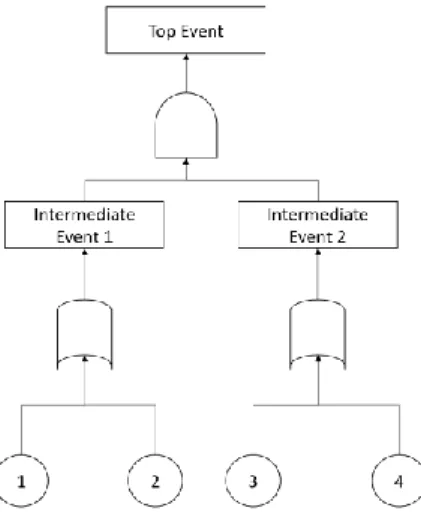
A fault tree is used to provide a visual top-down representation of cause to consequence analysis using Boolean logic. The undesired state of the system is termed as the top event. The causal factors contributing to the top event are classified as basic and intermediate events. Arcs and Boolean logic gates are used to connect basic events to intermediate events and then to top event (Panaitesco, 2018). An example of fault tree is shown in figure 2.

Figure 2:Representation of FT

In figure 2, basic events 1 & 2 are connected to intermediate event 1 through OR gate which means either basic event 1 or 2 must be true for intermediate event 1 to be true. Similarly, basic events 3 & 4 are connected to intermediate event 2 through OR gate. The intermediate events 1&2 are connected to the top event through AND gate, which implies both intermediate events must be true for the top event to be true.

(26)

14 2.8 Bayesian network

Bayesian network is used to represent the probabilistic graphical relationship between random variables. (J.Hulst, 2006).

The basis of BN is the Bayes’ theorem and is stated as (J.Hulst, 2006):

𝑃 (𝐴|𝐵) =𝑃(𝐵|𝐴)𝑋𝑃(𝐴)

𝑃(𝐵) (1)

Where,

𝑃(𝐴|𝐵) is the likelihood of A occurring, given B’s state of occurrence.

𝑃(𝐵|𝐴) is the likelihood of B occurring, given A’s state of occurrence.

𝑃(𝐴) is the likelihood of A occurring.

𝑃(𝐵) is the likelihood of B occurring.

The qualitative element of BN is represented by directed acyclic graph (DAG). Variables are represented as nodes and arc represents the causal relationship between the child node and the parent node.BN is quantified by using the conditional probability table (CPT). CPT defines the marginal probability of a variable dependent to another.

(27)

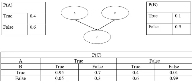
15 Figure 3: Example of BN

For example, in the above figure, A, B, and C are considered as the random variables where C is influenced by A & B. Here C is the parent node and A & B are child nodes. The CPT for C is defined which gives the probability of the hidden node given the parent node.

2.8.1 Network Structure

Consider ‘n’ stochastic random variables, X1, X2, X3……Xn in BN. If an arc points towards X2 from X1, then X1 is the child node, and X2 is the parent node. The joint probabilistic distribution 𝑃(𝑋1, 𝑋2, 𝑋3 … . . 𝑋𝑛) of the variables with state Xk is represented as follows (J.Hulst,

2006):

𝑃(𝑋1, 𝑋2, 𝑋3 … 𝑋𝑛) = ∏𝑛𝑘=1𝑝(𝑋𝑘|𝑃𝑎(𝑋𝑘)) (2)

Where,

(28)

16 2.8.2 Bayesian Probability

BN possess two important rules, i.e., expansion rule and chain rule which are discussed further.

2.8.2.1 Expansion rule

Consider 2 random variables X & Y, with j possible outcomes, then,

𝑃(𝑋) = 𝑝(𝑋|𝑦𝑗 _{= 1 ). 𝑝(𝑦}𝑗 _{= 1) + 𝑝(𝑋|𝑦}𝑗 _{= 2). 𝑝(𝑦}𝑗 _{= 2) + ⋯ + 𝑝(𝑋|𝑦}𝑗 _{= 𝑗). 𝑝(𝑦}𝑗 _{= 𝑗)}

=∑ 𝑝(𝑋|𝑌). 𝑝(𝑌)𝑌 (3)

In this rule, All the information of Y is ignored, and importance is given to only probability of X. This is also known as the marginal probability (J.Hulst, 2006).

2.8.2.2 Chain rule

The product rule is obtained by rewriting the Bayes’ theorem as follows

𝑃(𝑋, 𝑌) = 𝑝(𝑋|𝑌). 𝑝(𝑌) = 𝑝(𝑌|𝑋). 𝑝(𝑋) (4)

Consecutive application of product rule results in chain rule stated as follows

𝑃(𝑋1, … , 𝑋𝑛) = 𝑝(𝑋1) ∏𝑛_𝑖=2𝑝(𝑋𝑖|𝑋1, … . . , 𝑋𝑖 − 1) (5) Where,

X1, X2……Xi-1 is a subset of variable Xi. (J.Hulst, 2006)

2.8.3 Inference

Inference is updating the probability for a hypothesis as and when more evidence and information are known. For e.g., from figure 3, if the probability of A being ‘true' needs to be calculated given that C is true, then C is called the evidence variable and ‘A' as query variable. The equation used to calculate this inference of BN in the figure is as follows (J.Hulst, 2006):

𝑝(𝐴|𝐶) =𝑝(𝐶|𝐴)𝑋𝑝(𝐴)

(29)

17

Using the expansion rule and product rule, it can be re-written as

𝑃(𝐴|𝐶) = 𝑝(𝐶|𝐴𝑖). 𝑝(𝑖). 𝑝(𝐴)/ ∑ ∑ 𝑝(𝐶|𝐴𝑖). 𝑝(𝐴). 𝑝(𝑖)_𝐴 _𝐼 (7)

= (0.95𝑥0.1 + 0.7𝑥0.9)𝑥0.4/(0.95𝑥0.4𝑥0.1 + 0.4𝑥0.6𝑥0.1 + 0.7𝑥0.4𝑥0.9 + 0.01𝑥0.6𝑥0.9)

=0.91

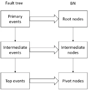
2.9 Mapping of a FT to BN

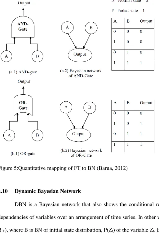
A fault tree is mapped to BN both qualitatively and quantitatively. In the qualitative step, the primary events, intermediate events and top events of fault tree are mapped to root nodes, intermediate nodes, and pivot nodes respectively in BN as shown in figure 4. The nodes in BN is connected in the same way as that of fault tree with the arcs. In the numerical step, the basic probabilities of the primary events in the fault tree are correspondingly assigned as prior probabilities of the nodes in BN (Khakzad, 2011). The primary events are associated with the intermediate events through AND-gate or OR-gate in a FT, and the equivalent mapping of these gates to BN using conditional probability table is shown in figure 5 (Barua, 2012).

(30)

18

Figure 5:Quantitative mapping of FT to BN (Barua, 2012)

2.10 Dynamic Bayesian Network

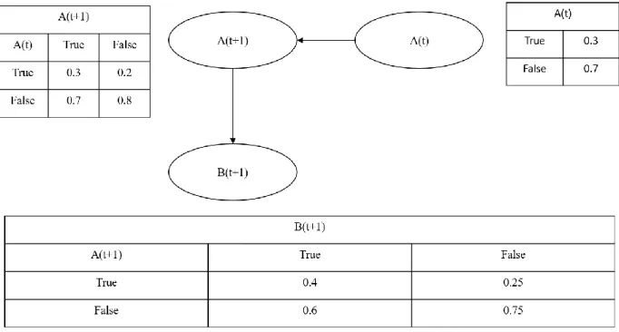
DBN is a Bayesian network that also shows the conditional relationship between time dependencies of variables over an arrangement of time series. In other words, it is defined as (B, B), where B is BN of initial state distribution, P(Zt) of the variable Zt. Bdefines the transitional

model P(Zt|Zt-1). Zt is represented as Zt= (Ut, Xt, Yt), where Ut, Xt, and Yt are input, hidden and

output variables of the model respectively (J.Hulst, 2006). The joint probability distribution of two-time slices is given as:

(31)

19

In DBN, the time-dependent relationship of nodes between 2-time slices are represented and is quantified using conditional probability table.

Figure 6:Example of DBN

In figure 6, the state of A at time ‘t+1' is conditionally dependent on the state of A at a time ‘t’ and the state of B at ‘t+1’ is influenced by the state of A at ‘t+1’.

(32)

20

CHAPTER III

DEVELOPMENT OF DBN

3.1 Research Methodology

The material of construction of pipe and electrochemical environment influences the internal corrosion rate. For an existing pipeline, the environmental condition varies over the length of the pipeline and changes with time (Muhlbauer, 2004). To combat the problem of the variation of risk over the distance, the pipe is segmented according to the similarity in electrochemical environmental characteristic, before performing the proposed risk assessment model which takes time variation of risk parameters into account.

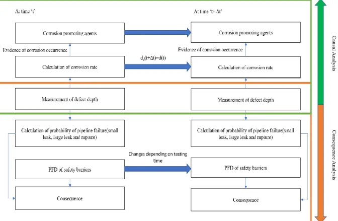
The visual representation of risk assessment model proposed is shown in figure 7. The corrosion promoting agents that contribute to internal corrosion are identified, and their relationships are represented using FT which is later converted to BN. The BN is then converted to DBN by establishing temporal dependence between the corrosion promoting agents of two different time steps using discrete nodes. The defect depths from inspection data are collected, and the corrosion rate is calculated. If the corrosion rate is greater than zero, then evidence that internal corrosion is ‘true' is provided in the internal corrosion node of DBN. Given the evidence, the posterior probability of corrosion promoting agents are computed to find out the causes of corrosion. The node with highest posterior probability is concluded to be the major causal factor for internal corrossion. The probability of LSFs (Limit State Functions) being less than zero and subsequent probability of failure of the pipeline is computed. Assuming the presence of ESD (Emergency Shutdown System) as a safety barrier, the overall probability of failure on demand is determined. Given the safety barrier and the probability of failure of the pipeline, the frequency of

(33)

21

consequence is calculated and analyzed. The temporal dependence of corrosion promoting agents, corrosion rate and safety barrier between two-time slices are established. This is shown in figure 7. The steps involved are further discussed in detail in the following subsections.

Figure 7:Framework for the pipeline internal corrosion model based on Dynamic Bayesian Network

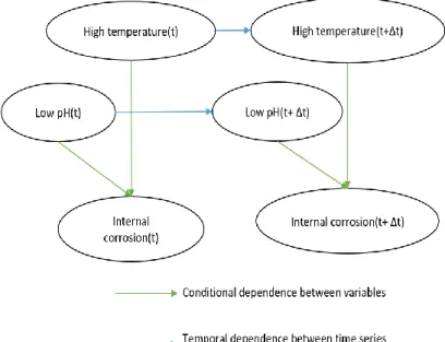
3.1.1 Corrosion promoting agents

In this model, the first step is to identify the corrosion promoting agents that contribute to the pipeline corrosion and to construct fault tree. The relationship between the corrosion promoting agents and corrosion along with temporal dependence between corrosion promoting agents between one-time step and the next time step is established as shown in figure 8. This is done in DBN by converting FT to BN and then to DBN using discrete nodes as discussed in the previous

(34)

22

chapter.After the calculation of internal corrosion rate, which is discussed in the next subsection, evidence of whether corrosion has occurred or not along with other evidence is given as input to investigate the causal factor. The variable which has the highest posterior probability is said to be the major contributor to the occurrence of corrosion.

Figure 8:Temporal dependence of corrosion promoting variables between adjacent time steps

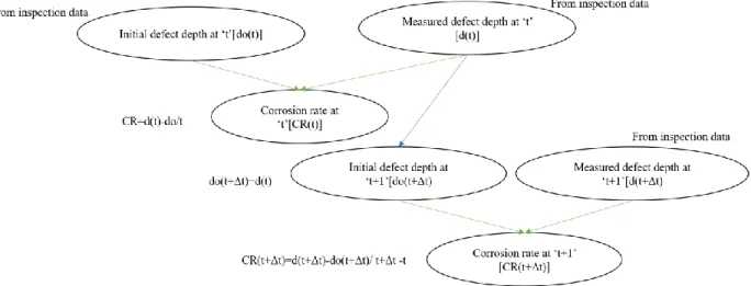
3.1.2 Calculation of internal corrosion rate

The defect depth after each inspection is collected. The defect depth is assumed to vary linearly and is calculated at each time step using the following equation (Khan,2014).

𝐶𝑅 =(𝑑(𝑡)−𝑑𝑜)

𝑡 (8)

Where,

𝐶𝑅 is corrosion rate

𝑑(𝑡) is the defect depth at time ‘t,' and

(35)

23

The temporal dependence of corrosion rate between the time slices is represented by equalizing the initial defect depth to the defect depth at previous time step. This can be visualized in figure 9.

Figure 9:Temporal dependence of corrosion rate between adjacent time steps

3.1.3 Calculation of probability of failure of the pipeline

Limit state function (LSF) is a condition beyond which the system/structure doesn't meet the design criteria. It is represented as the difference between load (L), on the system and resistance (R) of the system, to sustain the load. (Khan,2014)

𝑔 = 𝐿 − 𝑅 (9)

The probability of a small leak, large leak and rupture are then calculated using their respective LSF values. (Khan,2014)

• LSF1 for corrosion defect penetrating pipe wall(Khan,2014):

𝑔1(𝑡) = 𝑑𝑐 − 𝑑(𝑡) (10)

𝑑𝑐 = 0.8 ∗ 𝑤𝑡 (11)

(36)

24

𝑑𝑐 is critical defect depth.

𝑤𝑡 is wall thickness.

𝑑(𝑡) is defect depth at time ‘t.'

The critical defect depth is 80% of wall thickness (Khan, 2014). • LSF2 for plastic collapse under internal pressure(Khan,2014):

𝑔2(𝑡) = 𝑟𝑏𝑝− 𝑝(𝑡) (12)

Where,

𝑟_𝑏𝑝is resistance pressure to plastic collapse. 𝑝(𝑡) is internal operating pressure at time ‘t.'

According to failure pressure model standard DNV-RP-F101, rbp(t)= 2 ∗ t ∗ σu D−wt∗ [1 − d(t) wt]/[1 − ( d(t) Mwt)] (13) 𝑀 = √[1 + 0.31 ( 𝑙2 𝐷𝑤𝑡)] (14) Where,

σ_u is the ultimate tensile strength.

𝑀 is the folias factor or bulging factor that describes the connection between out of shape geometry of the deformed structure and defect parameters such as defect depth and defect length.

𝑙 is corrosion defect length of the pipeline.

𝐷 is the diameter of the pipeline. • LSF3 for rupture (Amin, 2012):

𝑔3(𝑡) = 𝑟_𝑏𝑝− 𝑝(𝑡) (15)

(37)

25 𝑟𝑏𝑝= 2𝑤𝑡𝜎𝑓 𝑀𝐷 (16) 𝑀 = (1 + 0.6275 ∗ 𝑙2 𝐷𝑤𝑡− 0.003375 𝑙4 𝐷2_𝑤𝑡2) 0.5 _for 𝑙2 𝐷𝑤𝑡≤ 50 (17) 𝑀 = 0.032 𝑙2 𝐷𝑤𝑡+ 3.3 for 𝑙2 𝐷𝑤𝑡> 50 (18) Where,

𝑟_𝑏𝑝 is resistance pressure for rupture

𝜎_𝑓 is flow stress of pipe

• Probability of LSF(g) being less than 0:

Probability of failure=𝑃𝑟(𝑔 < 0) (19)

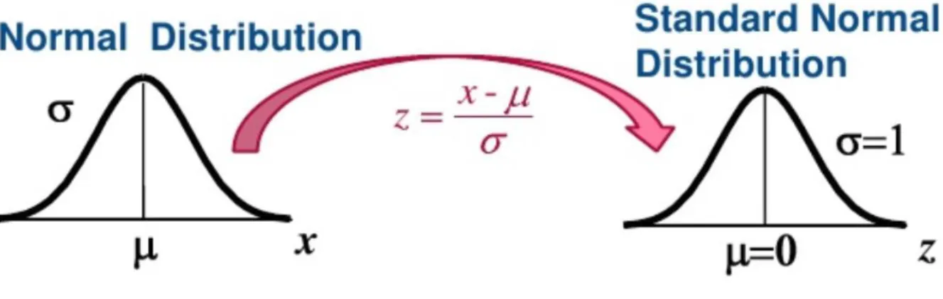
The normal distribution is converted to the standardized normal distribution that has a mean of 0 and standard deviation of 1 as shown in figure 10.

𝑃𝑟(𝑔 < 0) = 𝜑(𝑧) (20)

𝑧 =𝑥−𝜇𝑔

𝜎𝑔 (21)

Where x is the value being targeted in the normal distribution, i.e., 0 in this case. 𝜇_𝑔 and

𝜎𝑔are mean and standard deviation of the LSF’s normal distribution. z is the equivalent value in the standardized normal distribution for x. The area under the graph beyond the z value is the probability of LSF being less than zero and can be obtained from z-chart.

(38)

26

Figure 10: Conversion of normal distribution to standard normal distribution (Arora, 2011)

• Probability of failure of pipeline:

The failure of pipeline can be classified as a small leak, large leak, and rupture based on the combinations of LSF equations being less or more than zero. So, probability of a small leak, large leak, and rupture at time ‘t' can be defined as follows. (Amin, 2012)

Probability of small leak:

𝑃𝑠𝑙(𝑡) = 𝑃𝑟𝑜𝑏[𝑔1(𝑡) ≤ 0ꓵ𝑔2(𝑡) > 0] (22)

Probability of large leak:

𝑃_𝑙𝑙(𝑡) = 𝑃𝑟𝑜𝑏[𝑔1(𝑡) > 0ꓵ𝑔2(𝑡) ≤ 0)ꓵ𝑔3(𝑡) > 0] (23) Probability of rupture:

𝑃_𝑟𝑝(𝑡) = 𝑃𝑟𝑜𝑏[𝑔1(𝑡) > 0ꓵ𝑔2(𝑡) ≤ 0ꓵ𝑔3(𝑡) ≤ 0] (24) The overall probability of failure of the pipeline can be calculated as:

𝑃𝑂𝐹 = 1 − (1 − 𝑃𝑠𝑙)𝑥(1 − 𝑃𝑙𝑙)𝑥(1 − 𝑃𝑟𝑝) (25)

(39)

27 Figure 11: Calculation of POF of pipeline

3.1.4 Safety Barrier

The safety barrier is a physical/non-physical protective mean used to anticipate, prevent, control, and mitigate undesired events or incidents (Sklet, 2006). The safety barrier considered in this study is an automatic ESD.

The probability of failure on demand (PFD) of all the components in an ESD is calculated according to the voting architecture. Voting architecture is the design decision of a safety instrumented system (SIS) and is represented as MooN (M out of N) where M represents the minimum number of channels required to perform the Safety Instrumented Function(SIF), and N represents the total number of channels (Hearn, 2017). Table 1 shows the simplified Markovian equations for PFD calculation of different voting architecture (Hearn, 2017).

(40)

28

Table 1: PFD calculations for each voting architecture (Hearn, 2017)

Voting Architecture PFD equation

1oo1 𝜆𝑇𝐼 2 1oo2 𝜆2𝑇𝐼2 3 2oo2 𝜆𝑇𝐼 2oo3 𝜆2𝑇𝐼2 Where,

𝜆_𝐷𝑈 is dangerous undetected failure rate

𝑇𝐼 is the testing time interval

The overall PFD of a safety barrier is the sum of the PFDs of all its components.

𝑃𝐹𝐷_𝐸𝑆𝐷=∑ PFDi𝑛_𝑖 (26)

The dynamic change in the reliability of safety barrier is demonstrated by applying a condition of whether the components are tested within the proof test interval (TI suggested by the industry/standard). PFD remains the same when the components of ESD are tested regularly within the test time interval of proof test, and it varies with irregular testing. When the PFD is not tested within recommended test interval, then the PFD varies according to test time of whenever the components of ESD system is tested.

3.1.5 Consequence

Three consequences are defined based solely on the reliability of pipeline and the ESD system as follows:

(41)

29 Table 2: Definition of different consequences

Consequences POF of pipeline State of ESD system

C1 No loss of containment; state remains safe

0 Failure/Success

C2 Limited loss of containment >0 Success

C3 High loss of containment >0 Failure

 No loss of containment; occurs when the POF (Probability of Failure) of the pipeline is 0.

 Limited loss of containment; occurs when there is a pipeline failure, and the safety barrier succeeds in its function.

 Huge loss of containment; occurs when both the pipeline and safety barrier fail.

The overall PFD of the ESD system is calculated as discussed in the previous section. Given that the POF of pipeline is greater than 0 and depending on the failure or success of safety barrier, the frequency of consequence is represented and calculated using an event tree as shown in figure 12.

(42)

30 3.2 Software

There are various existing software programs used to develop DBN model. Bayes Net Toolbox for Matlab has most of the functionality required to develop DBN, but it is slow at processing, lacks Graphical User Interface (GUI) and has a conventional definition of DBN. Bayeslab and Netica have good GUI but unfortunately, lack functionality and are quite slow, making it difficult to solve complex problems. GENIE software is said to possess the, best of two worlds. It's GUI provides easy accessibility to core functionalities, and it also possesses rapid processing (J.Hulst,2006). GENIE was developed by decision system laboratory at the University of Pittsburgh (Bayesfusion, 2016). It allows representation of Object Oriented Network (OON), discussed in section 3.3 as OODBN, supports the use of both discrete and continuous variables, establishes temporal dependencies between variables and has cross compatibility with other dynamic Bayesian network models. GENIE can be downloaded for free for academic users from https://download.bayesfusion.com/files.html?category=Academia and the manual is available at http://support.bayesfusion.com/docs/genie.pdf. (Bayesfusion, 2016).

GENIE 2.2 is the latest version of GENIE software that supports a hybrid model which allows representation of dependencies between both discrete and continuous variable which is used for this research.

3.3 Visual representation of model using OODBN

To facilitate construction of DBN and to obtain a clear visualization, the overall model is mapped to an OODBN as shown in figure 13. OODBN simplifies the complexity, updates algorithm and probability effectively and can model repetitive sub-networks with ease. The OODBN consists of sub-networks of BN with normal nodes and interface nodes where normal

(43)

31

nodes are used to represent the relationship between two nodes and the interface nodes are used for communication between the sub-networks (Renninger).

(44)

32

CHAPTER IV

CASE STUDY AND RESULT

According to experts, crude oil pipelines are said to face a major threat due to internal corrosion (NACE, Managing Corrosion Of Pipelines That Transport Crude Oils, 2013). Therefore, crude oil flowing through a transmission pipeline of carbon steel 316 is considered for this study. The pipeline is segmented according to the similarity in electrochemical environment and operating conditions. Given the same pipeline material and operating conditions, risk assessment is carried out for a selected segment. Inspection is assumed to be carried out every two years with measured flaw depths of 5.5,6.5,7.5,8.5,9.5,10.5,11.5,12.5,13.5 mm for 9-time steps and an initial flaw depth of 4.5mm. Therefore, the time-interval considered to carry out risk assessment is 2 years. Other information about pipeline parameters is presented in table 3.

(45)

33

Table 3: Pipeline parameters used in the case study (Khan,2014)

Variable Unit Mean Std

deviation Distribution Internal Pressure P MPa 6.7 0.7 Normal distribution Diameter D Mm 600 18 Normal distribution Thickness T Mm 14 0.07 Normal distribution Pipe yield strength σy MPa 423 28 Normal distribution Pipe ultimate tensile strength σu MPa 550 36 Normal distribution Initial corrosion depth Do Mm 4.6 1.1 Normal distribution Initial corrosion length Lo Mm 200 4 Normal distribution Corrosion depth rate

Drate mm/yr 0.2 0.04 Normal

distribution Corrosion

length rate

Lrate mm/yr 20 4 Normal

distribution

The model is developed based on the following assumptions:

 Sweet corrosion takes place with the constant increase in CO2, H2O. with a probability of

80%. All other corrosion promoting agents have an equal probability of change with time.

 Micro-organisms in the pipeline are absent.

 The operating conditions and pH remains the same over time.

 Steady state flow is maintained in the pipeline.

 The internal corrosion rate varies linearly following the equation CR=d(t)-do/t.

 Emergency shutdown system is installed as a safety barrier with its components following 1oo1 architecture.

(46)

34

 Organizational factors and human factors are absent.

 The sensors are sensitive and can detect a leak of any magnitude, and false detection is absent.

 The consequence is categorized solely based on the failure of pipeline and success/failure of the ESD system.

4.1 Developing discrete DBN

A fault tree is constructed for internal corrosion in subsea as shown in figure 14, the top-event being the occurrence of internal corrosion and the basic events being the corrosion promoting agents of internal corrosion. The following corrosion promoting agents are identified as the causal factors contributing to internal corrosion(Khan,2016):

 Presence of O2  Presence of CO2  Presence of H2S  Presence of water

 Inhibitor failure

 Internal coating failure

 Poor pigging performance

 Internal large stress

 External large stress

 Residual stress

(47)

35

The basic probabilities for the corrosion promoting agents are assigned as shown in table 4. These probabilities are taken from the literature (Khan,2016).

(48)

36

Table 4: Probability of primary events in FT (Khan,2016)

Basic event Probability of occurrence

X1 Presence of O2 9.77E-03

X2 Presence of CO2 5.00E-03

X3 Presence of H2S 7.15E-03

X4 Presence of water 5.00E-03

X5 Inhibitor failure 6.23E-03

X6 Internal coating failure 7.74E-03

X7 Poor pigging performance 4.23E-03

X11 Internal large stress 5.50E-03

X12 External large stress 2.7E-03

X13 Residual stress 2.0E-02

X14 Stress concentration 7.26E-03

The fault tree is then mapped to BN at time ‘t,' with discrete nodes, with prior probabilities of root nodes same as that of probability of primary events in FT. The discrete nodes consist of 2 states i.e. ‘true’ and ‘false’. ‘true’ meaning the presence of variable in dangerous range that can contributes to corrosion and ‘false’ meaning presence of variable in safe range. The representation of BN is as shown in figure 15.

(49)

37 Figure 15: Framework of static BN

To develop a DBN, the root nodes at time ‘t’ and ‘t+2' are connected to each other with an arc representing the temporal dependence between the two BN. This is shown in figure 16. The DBN is quantified using conditional probability table of events at ‘t+2' with respect to the occurrence of events at a time ‘t' as shown in tables 5,6 &7 based on the assumption that CO2 and

(50)

38

Table 5: Conditional probability table of other corrosion promoting agent at ‘t+2’ Other corrosion promoting agents(t+2)

Other corrosion promoting agents(t)

True False

True 0.5 0.5

False 0.5 0.5

Table 6: Conditional probability table of H2O agents at ‘t+2’

Other corrosion promoting agents(t+2) Other corrosion promoting

agents(t)

True False

True 0.5 0.5

False 0.5 0.5

Table 7: Conditional probability table of CO2 at ‘t+2’

Presence of CO2(t+2)

Presence of CO2(t) True False

True 0.8 0.1

False 0.2 0.9

(51)

39

4.2 Calculation of corrosion rate and probability update

Equation 8 is implemented in the equation node, corrosion rate(t) of the model as shown in figure 17. The equation node calculates the internal corrosion rate and was found to be 0.2 mm/year at every time step, since the defect depth increases constantly for 1mm/yr.

Figure 17: Representation of interdependencies between equation nodes for corrosion rate calculation

Since the corrosion rate is greater than zero, an evidence of internal corrosion occurrence being true is given to the internal corrosion node. Posterior probabilities are then computed at every time step. Table 8 and table 9 shows the posterior probabilities at time ‘t’ and subsequent time steps respectively.

(52)

40

Table 8: Posterior probability for corrosion promoting agents at time ‘t’.

Basic event Posterior Probability

(Evidence as IC=’True’) X1 Presence of O2 0.449 X2 Presence of CO2 0.23 X3 Presence of H2S 0.328 X4 Presence of water 1 X5 Inhibitor failure 0.134 X6 Internal coating failure 0.159 X7 Poor pigging performance 0.004 X11 Internal large stress 0.118 X12 External large stress 0.019 X13 Residual stress 0.431 X14 Stress concentration 0.156

(53)

41

Table 9: Posterior probability for corrosion promoting agents for all the time steps except at time ‘t’

Basic event Posterior probability

(Evidence as IC=’True’) X1 Presence of O2 0.613 X2 Presence of CO2 0.32 X3 Presence of H2S 0.613 X4 Presence of water 1 X5 Inhibitor failure 0.508

X6 Internal coating failure 0.508 X7 Poor pigging performance 0.508 X11 Internal large stress 0.508 X12 External large stress 0.508

X13 Residual stress 0.508

X14 Stress concentration 0.508

From the computation of posterior probabilities, it has been observed that water is the major causal factor leading to corrosion at all time steps and measures must be taken to remove the water content from the pipe after which the major causal factor is presence of oxygen.

(54)

42 4.3 Calculation of POF of pipeline

Limit State Function equations are used to calculate the POF of pipeline due to a small leak, large leak, rupture and then the overall probability of failure of the pipeline by implementing equations 3 to 16 in the model using equation node as shown in figure 18.

Figure 18: BN framework representing the calculation of probability of failure of pipeline

Figures 19,20,21,22 show the estimated probability of LSFs being less than 0 and the overall probability of failure of pipeline respectively over additional time interval from initial time ‘t’.

(55)

43 Figure 19: Probability of LSF1 being less than 0

Figure 20: Probability of LSF2 being less than 0 0 0.2 0.4 0.6 0.8 1 1.2 0 2 4 6 8 10 12 14 16 18 p (g1 <0) Years 0 0.2 0.4 0.6 0.8 1 1.2 0 5 10 15 20 p (g2 <0) Years

(56)

44 Figure 21: Probability of LSF3 being less than 0

Figure 22: POF of pipeline

4.4 PFD calculation of ESD system

The ESD system is considered as the safety barrier used in this study. The ESD consists of a pressure sensor, 2 mass flow sensors, logic solver solenoid actuator and an isolation valve. Pressure sensors are commonly installed to monitor the pressure in the pipeline, so it's natural to use them for detecting a leak. The occurrence of a pipeline leak results in pressure drop. A lower

0 0.2 0.4 0.6 0.8 1 1.2 0 5 10 15 20 p (g3 <0) Years 0 0.2 0.4 0.6 0.8 1 1.2 0 5 10 15 20 POF o f p ip eline Years

(57)

45

limit pressure below operating pressure is set, and if the pressure drops below the setpoint, trip is initiated. A pressure sensor's sensitivity depends on leak location (Geiger). Therefore, flow monitoring using two mass flow sensors that operate on balancing method is recommended. Balancing method uses mass conservatism principle i.e., the mass of the fluid entering the pipeline at a particular time difference, Δt is the same as the fluid exiting the pipeline at the same time interval Δt. Flow sensors are installed at both inlet and outlet of the pipeline (Geiger). Flow is monitored for change and a trip is initiated, if the value contradicts the mass conservatism principle. The logic solver converts the analog input signal received by the sensors to a digital signal which is sent to the actuator. As the logic solver processes the analog signal sent by these sensors, it decides according to the pre-defined logic by the user. If the nature of the signal is found to be abnormal and is not in accordance to user's definition of the safe state, the output signal changes the Boolean value accordingly and is sent to the solenoid actuator. The solenoid actuator then de-energizes and closes the isolation valve, shutting down the pipeline. Figure 23 shows the workflow of components in an ESD system. The logic solver, actuator and shutoff valve are assumed to follow 1oo1 architecture. For a more effective system, the pressure sensor and both mass flow sensors are assumed to follow 1oo1 architecture. Both mass flow sensors are considered as one component that follows1oo1 architecture since they work on mass conservatism principle and are not redundant systems.

(58)

46 Figure 23: Workflow of components in ESD system

The overall PFD of the ESD system is calculated as follows: PFD avg=(1 2𝑥𝜆𝑃𝑆𝐿𝑥𝑇𝐼𝑃𝑆𝐿) 𝑥( 1 2𝑥(𝜆𝑀𝐹𝑆1+𝜆𝑀𝐹𝑆1)𝑥𝑇𝐼𝑀𝐹𝑆))+( 1 2𝑥𝜆𝐿𝑆𝑥𝑇𝐼𝐿𝑆) + (1 2𝑥𝜆𝐴𝑥𝑇𝐼𝐴)+( 1 2𝑥𝜆𝐼𝑉𝑥𝑇𝐼𝐼𝑉) (18)

The test time interval of all the components is 3 years the and values for dangerous failure rates of the components of ESD system is shown in table 10.

(59)

47 Table 10: Estimation of PFD of ESD system

Assuming that, the ESD system was not tested within the testing time interval of 3 years and was tested after 4 years at a time ‘t+12' and ‘t+18', the overall PFD increases at those time steps. From ‘t’ to ‘t+10’ the POF of pipeline is 0. Therefore, there is no loss of containment which implies that the frequency of C1=1 and C2=C3=0. Given, the POF of pipeline is greater than 0, and the PFD of ESD system from time ‘t+12’ and to ‘t+18’, the frequency of C2 & C3 are calculated, and the results are as shown in the table 11.

Table 11: Frequencies of consequences C2 and C3

From the results, it has been observed that frequency of high loss of containment is the highest at time ‘t+18’ due to the following reasons:

(60)

48

 Non-compliance to follow testing of safety barrier components within the test time interval recommended by the manufacturer resulting in increased PFD.

Whereas, frequency of limited loss of containment is highest at ‘t+12’ since the POF pipeline is comparatively low though the safety barrier is not tested according to recommended practice. The POF of pipeline is zero from time ‘t’ to ‘t+10’ and hence there is no loss of containment during that time span.

(61)

49

CHAPTER V

CONCLUSION AND FUTURE WORK

This research has an application to carry out a risk assessment for pipeline internal corrosion after inspection of a known time interval of defect depth. Given the defect depth, this model can help in investigating the causes of corrosion and also predict the consequence due to corrosion while dealing with the dynamic dependence of corrosion promoting agents and changing corrosion rate. This model also helps in visualizing the varying impact of irregular testing of safety barrier, given the probability of failure of pipeline on the consequence. A discrete DBN is used to represent the relationship of corrosion promoting agents with internal corrosion and their relationship between the two-time slices. The corrosion rate is calculated using the linear corrosion rate equation. Changing corrosion rate over time is depicted with changing defect depth after inspection. The possibility of a small leak, large leak and rupture are found out using LSF equations at each time step. The dynamic change in the probability of failure on demand of safety barrier depends on the testing time interval. If the components of safety barrier are tested within the regular testing time interval complied by the industry, the PFD remains the same. Otherwise, the PFD changes according to the time when the components of safety barrier are tested. Three consequences are defined; No loss of containment, limited loss of containment and huge loss of containment. Given the probability of failure and changing reliability of safety barriers over time, the frequency of consequence is calculated and analyzed.

A case study was proposed that considers a transmission pipeline that carries crude oil in high consequence area. It was assumed that the inspection of defect depth is carried out once in every 2 years. Therefore, the time interval between the risk assessment process was 2 years and

(62)

9-50

time steps were considered. From the results, it had been observed that the primary causal factor for corrosion is the presence of water at every time-step. The possibility of pipeline getting deteriorated starts at time ‘t+12’ and adverse consequence can be expected at time ‘t+18' due to failure of pipeline and high PFD of the ESD system.

Future work is recommended as follows:

 To use non-linear corrosion rate model

 To use continuous variable instead of discrete variables for corrossion promoting agents

 To consider the human and organizational factor in the risk assessment model

 To use Weibull distribution to demonstrate failure rate of safety barrier

 Establish dynamic change of consequence

(63)

51

REFERENCES

A.Amirat. (2006). Reliability assessment of underground pipelines under the combined effect of active corrosion and residual stress. International journal of pressure vessels and piping, Volume 83,issue 2, pages 107-117.

Amin, M. A. (2012). Bayesian Analyses of Metal-Loss Corrosion on Energy Pipeline Based on Inspection Data.

Arora, M. (2011, Sep 19). Linkedin. Retrieved from https://www.slideshare.net/raj_2952/normal-distribution-and-sampling-distribution

Barton, L. (2017). Offshore Oil and Gas Pipeline – Flow Assurance and Corrosion Modelling for Inspection Prioritization. Proceedings of the ASME 2017 India Oil and Gas Pipeline Conference.

Barua, S. (2012). Dynamic operational risk assessment with BN. College station: OGAPS. Bayesfusion. (2016). Bayesfusion,LLC. Retrieved from https://www.bayesfusion.com/ Berman, M. Y. (1994). Improving the Safety of Marine Pipelines.

Bertuccio. (2012). Risk assessment of corrosion in oil and gas pipelines using fuzzy logic. Corrosion Engineering Science and Technology.

Bhandari, J. (2016). Reliability Assessment of Offshore Asset under Pitting Corrosion using Bayesian Network. NACE.

Bharadwaj, A. (2014). Internal Corrosion of Pipeline. Alpha Science.

Chaves, I. A. (2014). Estimation of failure probability in corroded oil pipeline through monte-carlo simulation method applying the bootstrap technique. International Journal of Applied Science and Technology, Vol. 4, No. 5;.

(64)

52

Cheng, F. Y. (2013). Risk Assessment and Failure Prediction of High-Strength Steel Pipelines in the Presence of Corrosion Defects, Internal Pressure and Soil-Induced Strain.

International Offshore And Polar Engineering. Calgary.

Cobanoglu, M. (2016). Statistical Modeling of Corrosion Failures in Natural Gas Transmission Pipelines.

Corrosionpedia. (2018). Retrieved from

https://www.corrosionpedia.com/definition/2841/internal-corrosion Datta, K. (n.d.). A Corrosion Risk Assessment Model For Underground Piping .

David L. Slayter. (2008). Development of a GIS database of corrosion hazards for use in pipeline integrity assessment. Calgary: 7th International Pipeline Conference. Exida. (2017). Failure modes,effects and diagnostic analysis. Boulder: Exida.

F.Ayello. (2014). Quantitive Assessment of Corrosion Probability—A Bayesian Network Approach.

Fatmala, N. (2016, February 3). Retrieved from http://nfatmala.blogspot.com/2016/02/offshore-pipeline-corrosion-prevention.html

Gartland, P. O. (2003). Application of Internal Corrosion Modeling In the Risk Assessment of Pipelines. Norway: Corrosion.

Geiger, G. (n.d.). Principles of leak detection. krohne.

Groeger, L. (2012). Pipelines Explained: How Safe are America's 2.5 Million Miles of Pipelines? propublica.

Hearn, W. (2017). SIS implementation. Houston: SIS TECH.

J.C. Velázquez, *. (2009). Predictive Model for Pitting Corrosion in Buried Oil. J.Hulst. (2006). Modeling Physiological Processes with Dynamic Bayesian Networks.

(65)

53

K.McCallum. (2014). Localized Corrosion Risk Assessment Using Markov Analysis.

K.Younsi. (2013). Pipeline Integrity Assessment Using Probabilistic Transformation Method and Corrosion Growth Modeling Through Gamma distribution .

Khakzad, N. (2011). Safety analysis in process facilities: Comparison of fault tree and Bayesian network approaches. Reliability engineering and system safety, 925-932.

Khan, F. (2014). Application of Probabilistic Methods For Predicting The Remaining Life. 2014 10th International Pipeline Conference. Calgary.

Khan, F. (2015). Methods and models in process safety andrisk management: Past, present and future. Process safety and environmental protection, 116-147.

Khan, F. (2016). corrosion induced failure analysis of subsea pipeline. Elsevier, 214-222. Khan, F. (2017). Corrosion induced failure analysis of subsea pipelines. Reliability Engineering

and System Safety, Vol 159,Pg 214-222.

Maintaining the integrity of the marine pipeline network. (1994). In N. r. council, Improving the safety of marine pipeline (pp. 45-65). The National Academia Press.

Melchers, R. (2003). Modeling of marine immersion corrosion for mild and low alloy steels-part 1:Phenomenological model. Corrosion section.

Muhlbauer, W. (2004). Pipeline Risk Management Manual: Ideas, Techniques, and Resources. Elsevier.

NACE. (2000). Corrosion Failures: El Paso Natural Gas Pipeline Explosion. NACE. NACE. (2013). Corrosion Failures: Sinopec Gas Pipeline Explosion. NACE.

NACE. (2013). Managing Corrosion Of Pipelines That Transport Crude Oils. Pipeline oil & gas journal, Vol. 240, No.3.