Panel Data Estimation Techniques for Farm-level Data Model
*
Platoni S., Sckokai P. and Moro D.
Istituto di Economica Agro-alimentare, Università Cattolica, 29100 Piacenza, Italy
* This research has been carried out as part of the WEMAC (World Econometric Modelling of Arable Crops) research project (Scientific coordinator: Catherine Benjamin), funded by the European Commission under the 6th Framework programme. The FADN data have been
provided in the context of that project.
Abstract - Econometric models wishing to estimate relevant parameters for agricultural policy analysis are increasingly relying on unbalanced panels of farm-level data. Since in the agricultural economics literature such models have often been estimated through simplified approaches, in this paper we try to verify whether the adoption of more sophisticated panel data techniques may impact the estimation results. For this reason, the policy model by Moro and Sckokai (1999) has been re-estimated using techniques recently developed in the econometric literature. The preliminary results show a strong impact on the estimations. This seems to suggest that the adoption of proper panel-data techniques is likely to be very important in order to obtain reliable estimates of some key policy parameters.
Keywords- Agricultural policy, Panel data, Systems of equations
I. INTRODUCTION
Econometric models wishing to estimate relevant parameters for agricultural policy analysis are increasingly relying on farm-level data, like the Farm Accounting Data Network (FADN - EU) or the Agricultural Resource Management Survey (ARMS - US). The structure of these databases is quite similar, since they are typically unbalanced panels, where we find repeated information on some farms but the same farm may not enter the sample every year. Moreover, they typically collect data referring to a large number of farms, providing very detailed information on farm production activities as well as on farm structural characteristics and resource use.
In recent years, a number of papers have been published drawing relevant policy implications from the estimation of arable crop supply/acreage equations carried out on these databases, either related to the EU Common Agricultural Policy (CAP) (see, e.g., Oude
Lansink and Peerlings (1996), Oude Lansink (1999), Moro and Sckokai (1999), Sckokai and Anton (2005), Serra et al. (2005), Sckokai and Moro (2006) and Serra et al. (2006)) or to the corresponding US policy (see, e.g., Goodwin and Mishra (2006)). However, these papers have always adopted a simplified approach in taking into account the complex econometric issues implied by the use of these databases. In fact, their use implies the adoption of proper panel-data techniques suitable for system of equation estimation, in which the issue of censoring is properly taken into account, since it is very common that not every farm produces each crop every year.
In light of these considerations, the present paper re-examines the analyses proposed for Italy by Moro and Sckokai (1999), adopting a more suitable econometric approach. Thus, we model the CAP arable crop regime using FADN data for Italy in order to analyse supply and acreage response to policy parameters, under the maintained hypothesis of risk-neutral behaviour by farmers. This empirical application has mainly illustrative purposes, since the main objective of the paper is to underline the different results obtained adopting different panel data techniques.
In terms of econometric approach, the paper relies on the Error Component Model (ECM), which is the most frequently used approach to analyse panel data in econometrics. When the panel is incomplete, which is the rule rather than the exception when the data come from large-scale surveys, standard estimation methods cannot be applied (see, e.g., Wansbeek and Kapteyn (1989), Baltagi et al. (2001) and Davis (2002)). Hence the general model we consider is a two-way error component regression for unbalanced panel data, in which both firm and time effects are introduced (among recent empirical applications adopting this approach, see, e.g., Boumahdi et al. (2004)). We
present results obtained using both single equation and system of equation estimation techniques, in which censoring issues have been taken into account using a proper two-step approach.
II. MODEL
A. Theoretical model
The model we adopt refers specifically to the CAP for arable crops as it was implemented before the 2003
reform1. Under this package, farm income was
supported through three main policy tools: the intervention price for cereals, the crop-specific area payments, introduced with the 1993 reform of the CAP, and the compulsory rate of set-aside. Thus, any model wishing to analyse farmers’ response to these policy tools have to incorporate them in its assumed decision making structure.
As in Moro and Sckokai (1999), we consider the following profit function for the representative farmer:
(
)
(
s)
T s c 1 c s s s s t s ds s b c s d T p n 1 i i r T r n 1 k k r p n 1 i i i e n s 1 s T e ∈ + = ≤ + + + − ≡∑
∑
∑
= = = , , , , . . max , , , , , , ,..., , , s z x y x w' y ' p z b w p yx π(1)
where y is the n-dimensional vector of farm outputs
and pe is the corresponding vector of expected output
prices, x is the m-dimensional vector of variable inputs
and w the corresponding vector of input prices, s is the
vector of land allocations to the n crops, with sT being
total farm land, np<n is the number of crops included
in the arable crop regime, b is the vector of
crop-specific area payments, d is the set-aside payment, c is
the set-aside percentage, sr is the land that must be set
aside, z is the vector of quasi-fixed inputs in the short
run and T is the multi-output short-run technology.
Finally, the three constraints are the total land
1
As it is well known, the most recent reform of the CAP was implemented starting in 2005. Thus, reliable farm-level data referring to the application of the new Single Farm Payment scheme will become available only in the near future.
constraint, the set-aside constraint and the technological constraint, respectively.
If we assume that π
(
pe,w,b,d,sT,c,z)
is twicecontinuously differentiable, we can write the following set of derivative properties:
(
)
( )
(
)
( )
(
)
( )
p i T e i h T e h e i T e i n 1 i b c s d s m 1 h w c s d x n 1 i p c s d y ,..., , , , , , , ,..., , , , , , , ,..., , , , , , , = ⋅ = = ⋅ − = = ⋅ = δ δπδ δπ δ δπ z b w p z b w p z b w p (2)which allow us to define a set of output supply, input demand and land allocation equations that can be estimated on farm-level data. Since this model estimates simultaneously both supply and land allocation decisions, crop yields become endogenously defined.
B. Empirical specification
For a parametric specification of (1), we rely on the normalized quadratic function, a flexible functional form largely applied to the estimation of agricultural profit functions. This functional form has a Hessian of constants, so the curvature properties can hold globally. Moreover, it allows negative profits, which cannot be managed when logarithmic transformations
are used. Choosing pme as the numeraire, the
normalized quadratic profit function takes the following general form:
q A q q a′ + ′ + =a0 π (3) where e m p π π = , ⎟⎟ ⎠ ⎞ ⎜⎜ ⎝ ⎛ = s cz p p p e T m e m e m e , , , , ,w b p
q and the scalar
a0, the vector a and the matrix A are parameters to be
estimated.
Using the derivative property in (2), output supply, input demand and land allocation equations can be written as: 2 n m n 1 j 1 n m n m n i q s 2 n m n 1 j 1 m n 1 n h q x 2 n m n 1 j n 1 i q y p p j j ij i i p j j hj h h p j j ij i i + + + = − + + + = ⎟⎟ ⎠ ⎞ ⎜⎜ ⎝ ⎛ + = + + + = − + + = ⎟⎟ ⎠ ⎞ ⎜⎜ ⎝ ⎛ + − = + + + = = ⎟⎟ ⎠ ⎞ ⎜⎜ ⎝ ⎛ + =
∑
∑
∑
,..., ,..., ,..., ,..., ,..., ,..., γ γ β β α α(4)
where α’s, β ’s, and γ ’s are appropriate elements of
the above vector a and matrix A.
Due to the specification of the vector q, the
homogeneity property is maintained within the empirical model. Moreover, the standard symmetry and reciprocity properties can be imposed with the
following parametric restrictions: αij =αji, βhj =βhj
and γij =γji.
III. DATA
The data used for the present study are taken from the EU FADN database for the period 1994-2003 (ten years) and refer to the sample of Italian specialised arable crop farms. As mentioned in the introduction, the database is an unbalanced panel of 14,288 individuals observed in the above 10 years period, for
a total of 34,140 observations2.
The database provides most of the variables needed to estimate the model: crop productions, output prices, land allocations, area payments, family labour, hired labour (number of hours and hourly wages), variable input costs by category (seeds, fertilisers, chemicals, water …) and quasi-fixed input stock values (buildings and machinery). Variable input prices are not provided by the FADN; thus, price indexes for Italy have been taken from the official Eurostat statistics. The same has been done for deflating capital values, since Eurostat provides also time series of rental price indexes for capital goods.
The initial FADN dataset is very disaggregated, especially in terms of number of outputs and number of variable inputs; thus, to make the estimation feasible, some aggregation has been introduced. We have considered five output categories (durum wheat, maize, oilseeds, other cereals, and other arable crops) with their respective land allocations, where the first
2
The sample we have used was obtained after the elimination of those farms that presented some “severe outliers” in the key variables needed for the estimation. All farms showing output prices and crop yields falling out of the range defined by the sample mean and two standard deviations were eliminated. The general idea of this procedure is to eliminate those observations that are likely to come from some errors in plugging in the basic data.
four represent those crops for which the CAP arable crop regime guaranteed different levels of area payments. We have also considered two variable inputs (crop inputs and other variable inputs), one fixed input (total land) and one quasi-fixed inputs (aggregate of capital and family labour). The price of “other inputs” is our numeraire in the normalised quadratic specification. The aggregates have been generated as Laspeyres indexes, while short run profit has been computed as the sum of total gross sales and total area payments minus total variable costs.
Since output prices are unknown at the time land allocation decisions are made, an assumption on how price expectations are formed is needed. We have adopted the well-known “adaptive expectation” hypothesis, following the approach proposed by Chavas and Holt (1990), which implies a correction of
lagged prices3. Clearly, since our panel is incomplete,
individual (farm) lagged prices cannot be used to construct the series of expected prices. Thus, for each crop, yearly regional average prices have been computed and used to model the mechanism of price
expectations4.
IV. ECONOMETRIC TECHNIQUES
A. Censoring
As mentioned in the introduction, the estimation of supply and land allocation equations implies the adoption of an appropriate technique to account for censoring, since not every farm produces every crop each year. In order to obtain suitable results for policy analysis, this problem has to be addressed adopting a methodology that uses all the available observations, in order to preserve the representativeness of the FADN sample. For this reason, we used the two-step estimation procedure proposed by Shonkwiler and
3
This correction is based on the assumption that, in each period, farmers update their “naive” expectations (lagged prices) based on the past history of the observed differences between actual prices and “naive” expected prices.
4
To avoid the problem of eliminating entire years to model lagged prices, we have used national crop prices taken from Eurostat to model expectations in the first years of our sample.
Yen (1999). Thus, the system of equations in (4) is estimated in the following form:
(
∗)
(
)
+(
∗)
= it i i it i i it i it Φ h,η f q ,ψ ρΘh,ην (5)
where hit is a vector of variables which explains the
binary choice of producing/non producing crop i and
* i
η are first-stage probit estimates of the corresponding
parameters; νit is any of the dependent variable and
( )
⋅i
f is any of the equations of the system in (4); ψi is
the subset of the normalized quadratic parameters to
be estimated that enter equation fi
( )
⋅ ; Φ(⋅) and Θ(⋅)are the univariate standard normal cumulative distribution and probability density functions, respectively, both computed over probit results, while
i
ρ is an extra parameter to be estimated.
The five probit models (one for each output) are estimated using as explanatory variables the level of three quasi-fixed inputs (family labour, buildings and machinery) and one set of dummy variables
representing different regions/altitudes5. Thus, in each
probit model we estimated 10 parameters.
B. Panel data estimation
The panel data estimation relies on the error component model (ECM), which is the most frequently used approach to analyse panel data in econometrics. Since the panel is incomplete, standard estimation methods cannot be applied (see, e.g., Wansbeek and Kapteyn (1989), Baltagi et al. (2001), Davis (2002) and Boumahdi et al. (2004)).
At first, we have estimated our model using the standard single equation one-way fixed effect (FE) and one-way random effect (RE) models, for which estimation commands exist in the most common econometric softwares. As it is well known, one-way FE and RE models assume that differences across individuals can be captured by means of an individual specific intercept term. The FE approach considers
5
Other pertinent variables to be included in probit estimation would be soil quality or demographic characteristics of the farmer (age, education, …), but unfortunately these variables are not included in the FADN database.
this term as a fixed parameter, while the RE approach
considers it as a random disturbance6.
In addition, we have estimated a set of two-way RE and FE models, which explore simultaneously both differences across individuals and differences over time for each individual. The econometric software we use (TSP version 5.0) offers the possibility of estimating the Maximum Likelihood (ML) two-way RE model, but we have decided to build our own GLS estimator in order to compute the two-way Hausman
test (see Baltagi (2005)).
Note that, when adopting a two-way ECM approach, it is legitimate to consider only the individuals which appear at least twice, since individuals appearing only once do not add any useful information (Wansbeek and Kapteyn (1989)). Thus, after this elimination, our final sample is an unbalanced panel of 7,526 individuals observed in 10 years, for a total of 27,378 observations. In order to compare the results, we have used this reduced database also for one-way FE and RE estimation.
Single equation two-way ECM
The single equation two-way ECM estimation technique for unbalanced panel has been introduced by Wansbeek and Kapteyn (1989) and our estimator has been built following their procedure.
Our unbalanced panel is characterized by a total of
n observations, by F farms, indexed by i=1,...,F, and
by T periods, indexed by t=1,...,T. Let Ti denote the
number of times the farm i is observed and Ft the
number of farms observed in period t. Hence
n F T t t i i =
∑
=∑
.Let Dt be the
F
t×
F
matrix obtained from IF byomitting the rows corresponding to farms not observed
6
The one-way FE is the most common approach adopted in agricultural economic studies employing panel data estimation techniques (see, e.g., Oude Lansink and Peerlings (1996), Oude Lansink (1999), Sckokai and Anton, (2005)). Other studies adopt ad hoc simplified approaches, that do not explore specifically the panel structure of the data (see, e.g., Moro and Sckokai (1999), Sckokai and Moro (2006), Serra et al. (2005) and Serra et al. (2006)).
in period t. With =
(
′ ′)
′ ×F 1 T n1 D D Δ ... and(
tF)
T n2 diag Dι Δ = × we can define 1 1 F FF Δ Δ Δ ≡ ′ × , 2 2 T TT Δ Δ Δ ≡ ′ × and 2 1 F TTF Δ Δ Δ ≡ ′ ×and we can consider ⎟
⎠ ⎞ ⎜ ⎝ ⎛ ≡ × ×F nT n1 2 Δ Δ
Δ , which gives the
dummy-variable structure for the unbalanced panel model.
In the two-way FE model we consider the following
matrices:
(
)
(
[ ])
[ ](
TF)
2 2 [ ]1 2 1 F 1 2 2 TF 1 F TF T 2 1 2 1 n 2 1 1 F 1 n TF 1 F 1 2 Δ Q Δ Δ Δ Δ Δ Δ Δ Δ Δ Δ Δ Δ Q Δ Q Δ P I Δ Δ Δ Δ I Δ Δ Δ Δ Δ Δ Δ Δ ′ = ⋅ ′ = ′ − ⋅ ′ = ′ − ≡ = ⋅ − = ⋅ ′ − = ′ − ≡ − − − − (6) and hence the projection matrix onto the null-space ofΔ is: [ ]
(
1)
[ ]1 [ ]1 2 2 [ ]1 1 F 1 n Δ Δ Δ Δ I ΔΔ Δ ΔQ Δ Q Q ΔQ ΔQ Q = − − ′ − − ′= − − ′ (7) and therefore the within estimator is:[ ]
(
XQ X)
(
XQ[ ]y)
β = ′ Δ ′ Δ
−1
WT (8)
In the two-way RE model (GLS) the covariance
matrix of the composite error uit =μi+νt+εit is:
( )
2 2 2 1 1 2 n 2 Euu I ΔΔ ΔΔ Ω= ′ =σε +σμ ′+σν ′ (9) With 2 F 2 F F Δ I Δ μ ε σ σ + = ~ and 2 T 2 T T Δ I Δ ν ε σ σ + = ~ , by defining: [ ] I ΔΔ Δ Q Δ Δ Δ Δ Q Δ = − ′ ′ − = − − 1 F 1 n 1 TF 1 F TF T ~ ~ ~ ~ ~ (10) Wansbeek and Kapteyn (1989) show that:[ ] [ ] [ ]
(
1 1 2 2 1)
2 1 1 Δ -Δ Δ Q ΔQΔQ Q Ω− = ~ −~ ~ ′~ ε σ (11)and then the GLS estimator is:
(
XΩ X) (
XΩ y)
βGLS= ′ −1 −1 ′ −1 (12)
We derive Quadratic Estimations (QUEs) for σε2,
2
μ
σ and σν2 by using the FE residuals, averaged over
farms or averaged over periods. Since we are considering a constant term, with the FE residuals
WT Xβ
y
e≡ − and with f =En⋅e=e−e we equate:
[ ] f Δ Δ Δ f f Δ Δ Δ f f Q f Δ ′ ′ ′ = ′ ′ = ′ = − − 1 1 F 1 T 2 1 T 2 F n q q q (13)
to their expected values:
( )
(
)
( ) (
)
(
)
( ) (
)
(
2)
2 2 1 2 2 2 0 T T 2 2 2 1 2 2 2 0 F F 2 n F n 1 k k F q E n T 1 k k T q E k 1 F T n q E ν μ ν μ ε ν μ ν μ ε ε σ λ σ λ σ σ σ σ λ σ λ σ σ σ σ ⋅ + ⋅ − ⋅ + ⋅ + + ⋅ − − + = ⋅ + ⋅ − ⋅ + ⋅ + + ⋅ − − + = ⋅ − + − − = (14) with{
(
XQ[ ]ΔX)
XΔ Δ Δ2X}
1 -T 2 1 F tr k = ′ − ′ ′ , [ ](
)
{
XQΔX XΔΔ-1Δ1X}
F 1 1 T tr k = ′ − ′ ′ and [ ](
)
n k n 1 n 0 ι X X Q X X ι′ ′ Δ ′ = − and with n T n F 1 i 2 i n 1 1 n 1∑
= = ′ ′ = ι ΔΔι λ and n F n T 1 t 2 t n 2 2 n 2∑
= = ′ ′ =ιΔ Δι λ . If 0 x u E it it ≠ ⎟⎟ ⎠ ⎞ ⎜⎜ ⎝ ⎛then the estimator βGLS becomes
biased and inconsistent for β. Hausman (1978)
suggests comparing βGLS and βWT both of which are
consistent under the null hypothesis H₀: 0
x u E it it = ⎟⎟ ⎠ ⎞ ⎜⎜ ⎝ ⎛
but which will have different probability limits if H₀ is
not true. Baltagi (2005) asserts that the standard Hausman test performs correctly also in the two-way ECM. Therefore we compute:
WT GLS 1 β β
q =~ −~ (15)
where β~GLS and β~WT are the vectors of the estimated
parameters without the constant term andthe Hausman
test statistic is given by:
[ ]
(
) (
)
(
)
1 1 1 1 1 2 1 1 m q XQΔX XΩ X q − − − − ′ − ′ = 'σε ~ ~ ~ ~ (16)where X~ is the matrix of the regressors without the
constant term. Under H₀ the test m1 is asymptotically
distributed as χk~2 where k
~
denotes the dimension of
Two-way SUR system
The most appropriate way of estimating the model in (4) is by a system of equation estimation technique, which in this specific case must be a Seemingly Unrelated Regression (SUR) technique, which allows to impose cross equations restrictions. Once again, standard econometric softwares do not provide automatic commands to estimate two-way SUR systems, since estimating such system implies the adoption of a specific procedure for inverting the
variance-covariance matrix of the residuals Ω−1. This
procedure has been recently proposed by Biørn (2004) for the estimation of a one-way SUR system. Based on this framework, we have derived the corresponding estimator for the two-way SUR system.
Let consider a system of M equations, indexed by
m=1,…,M. The farms are observed in at least two
periods and at most T periods. Let F~p denote the
number of farms observed in p periods, with p=2,…,T.
Hence F F p p=
∑
~ and F p n p p =∑
~ . We assume thatthe farms are observed in T-1 groups such that the F2
~
farms observed twice come first, the F3
~
farms observed three times come second, etc. Hence with
∑
= = p 2 k k p FC ~ being the cumulated number of farms
observed up to p times, the index sets of the farm
observed p times can be written as
{
p1 p}
p C 1 C
I = − + ,..., where p=2,…,T and C1=0 (note
that Ip may be considered as a pseudo-balanced panel
with p observations of each farm).
With km being the number of regressors for equation
m, the total number of regressors for the system is
∑
= = M 1 m m SUR kk . Stacking the M equations for the
observation
( )
i, we have: t 1 Mit 1 SUR k SUR k M it 1 Mit 1 Mt 1 Mi 1 SUR k SUR k M it 1 M×it = × ×+ ×+ ×+ × = × ×+ × u β X ε ν μ β X y (17)where Xit =diag
(
x1it...xMit)
and(
)
′ ′ ′ =diag β1 βM β ... . With μi=
(
μ1i...μMi)
′, νt =(
ν1t...νMt)
′ and(
)
′ = 1tt Mit it ε ε ε ... , we assume:(
)
(
)
(
)
t t i i 0 t t i i E t t 0 t t E i i 0 i i E 2 mj t i j mit 2 mj tj mt 2 mj i j mi ′ ≠ ′ ≠ = ′ = ′ = = ′ ≠ = ′ = = ′ ≠ = ′ = = ′ ′ ′ ′ or and , , , ε ν μ σ ε ε σ ν ν σ μ μ (18) Hence 1 M×t μ , 1 M×t ν and 1 Mit×ε have zero expectations and
covariance matrices M M×μ Σ , M M×ν Σ and M M×ε Σ . It follows that M M t t i i M M t t M M i i 1 Mit 1 Mit E × ′ ′ × ′ × ′ ×′′ × + + = ⎟ ⎠ ⎞ ⎜ ⎝ ⎛ ′ ε ν μ δ δ δ δ Σ Σ Σ u u with δii' =1
for i=i' and δii' =0 for i≠i', δtt' =1 for t=t' and
0 δtt' = for t≠t'. Let us consider ( ) ′ ⎟ ⎠ ⎞ ⎜ ⎝ ⎛ ′ ′ = × × × 1M ip M 1 i1 1 pM p i y y y ... , ( ) ′ ⎟⎟ ⎠ ⎞ ⎜⎜ ⎝ ⎛ ′ ′ = × × × k M ip M k i1 k pM p i SUR SUR SUR X X X ... and ( ) ′ ⎟ ⎠ ⎞ ⎜ ⎝ ⎛ ′ ′ = × × × 1 M ip M 1i1 1 pM p i u u u ... for p I
i∈ and p=2,…,T (and then for
T 1 T 3 2 2,C 1,...,C ,...,C 1,...,C C 1,..., i= + − + with F CT = ).
We define the matrix ( )
TM pM p i × Δ indicating in which
period t the farm i is observed. For example with T=4
if the farm i is observed in t=2 and in t=4 we have
( ) ⎥ ⎦ ⎤ ⎢ ⎣ ⎡ = × M M TM pM p i ι 0 0 0 0 0 ι 0 Δ . Hence with ′ ⎟ ⎠ ⎞ ⎜ ⎝ ⎛ ′ ′ = × × ×1 1M1 1MT
TMν ν ...ν for the farm i∈Ip we can define
( ) ( ) TM 1 TM pM p i 1 pM p i × × × = Δ ν
ν and we can write the model:
( ) ( ) ( ) ( ) ( ) ( )
(
)
(
)
(
)
M M p pp M M p pp M M p pp M M p pp pM pM p 1 pM p i 1 SUR k SUR k pM p i 1 pM p i 1 pM p i 1 Mi 1 p p 1 SUR k SUR k pM p i 1 pM p i p × × × × × × × × × × × × × × × × × × × + + ⊗ + + ⊗ = = ⊗ + + ⊗ = + = + + ⎟ ⎠ ⎞ ⎜ ⎝ ⎛ ⊗ + = μ ν ε ν ε μ ν ε Σ Σ Σ J Σ Σ E Σ J Σ Σ I Ω u β X ε ν μ ι β X y (19)Since Ep and Jp are symmetric and idempotent and
have orthogonal columns we have:
(
)
(
)
M M 1 p pp M M 1 p pp pM pM 1 -p p × − × × − × × + + ⊗ + + ⊗ =E Σε Σν J Σε Σν Σμ Ω (20)Then we can consider the GLS problem for β when
μ
Σ , Σν and Σε are known, i.e. the problem of
minimizing: ( ) ( ) ( )
(
)
( ) ( )(
)
( )∑∑
∑∑
∑∑
= ∈ × − × = ∈ × − × = ∈ − ⎥⎦ ⎤ ⎢⎣ ⎡ ⊗ + + ′ + + ⎥⎦ ⎤ ⎢⎣ ⎡ ⊗ + ′ = ′ T 2 p iIp p i M M 1 p p p p i T 2 p iIp p i M M 1 p pp p i T 2 p iIp p i 1 p p i pΣ u Σ Σ J u u Σ Σ E u u Ω u μ ν ε ν ε (21)If we apply GLS on the observations for the farms
observed p times we obtain:
( ) ( ) ( ) ( ) ( )
[
(
)
]
( ) ( )[
(
)
]
( ) ( )[
(
)
]
( ) ( )[
(
)
]
( ) ⎥ ⎥ ⎥ ⎥ ⎦ ⎤ ⎢ ⎢ ⎢ ⎢ ⎣ ⎡ + + ⊗ ′ + + + ⊗ ′ × × ⎥ ⎥ ⎥ ⎥ ⎦ ⎤ ⎢ ⎢ ⎢ ⎢ ⎣ ⎡ + + ⊗ ′ + + + ⊗ ′ = = ⎥ ⎥ ⎦ ⎤ ⎢ ⎢ ⎣ ⎡ ′ × ⎥ ⎥ ⎦ ⎤ ⎢ ⎢ ⎣ ⎡ ′ =∑
∑
∑
∑
∑
∑
∈ × × − × ∈ × × − × − ∈ × × − × ∈ × × − × ∈ × × − × − ∈ × × − × × p I i pM pM pM1 1 p pM p I i pMpM pM1 1 p pM 1 p I i pMpM pMkSUR 1 p pM p I i pMpM pMkSUR 1 p pM p I i pM1 1 p pM 1 p I i pMkSUR 1 p pM 1 SUR k GLS p p p p i SUR k ip p i SUR k p i p i SUR k ip p i SUR k ip p i pM pM SUR k ip p i pM pM SUR k ip y Σ Σ Σ J X y Σ Σ E X X Σ Σ Σ J X X Σ Σ E X y Ω X X Ω X β μ ν ε ν ε μ ν ε ν ε (22)while the full GLS estimator is:
( ) ( ) ( ) ( ) ( )
[
(
)
]
( ) ( )[
(
)
]
( ) ( )[
(
)
]
( ) ( )[
(
)
]
( )⎥ ⎥ ⎥ ⎥ ⎦ ⎤ ⎢ ⎢ ⎢ ⎢ ⎣ ⎡ + + ⊗ ′ + + + ⊗ ′ × × ⎥ ⎥ ⎥ ⎥ ⎦ ⎤ ⎢ ⎢ ⎢ ⎢ ⎣ ⎡ + + ⊗ ′ + + + ⊗ ′ = = ⎥ ⎥ ⎦ ⎤ ⎢ ⎢ ⎣ ⎡ ′ × ⎥ ⎥ ⎦ ⎤ ⎢ ⎢ ⎣ ⎡ ′ =∑∑
∑∑
∑∑
∑∑
∑∑
∑∑
= ∈ × × − × = ∈ × × − × − = ∈ × × − × = ∈ × × − × = ∈ × × − × − = ∈ × × − × × T 2 p iIp pMpM pM1 1 p pM T 2 p iIp pMpM pM1 1 p pM 1 T 2 p iIp pMpM pMkSUR 1 p pM T 2 p iIp pM pM pMkSUR 1 p pM T 2 p iIp pM1 1 p pM 1 T 2 p iIp pMkSUR 1 p pM 1 SUR k p p p i SUR k ip p i SUR k ip p i SUR k ip p i SUR k ip p i pM pM SUR k p i p i pM pM SUR k p i GLS y Σ Σ Σ J X y Σ Σ E X X Σ Σ Σ J X X Σ Σ E X y Ω X X Ω X β μ ν ε ν ε μ ν ε ν ε (23)We can estimate the covariance matrices Σμ, Σν
and Σε by following either the within-between
procedure suggested by Biørn (2004) – corrected for the two-way model – or the QUE procedure suggested by Wansbeek and Kapteyn (1989) – corrected for the
SUR.
The first method considers the FE residuals
WT it 1 Mit Xβ y e ≡ − ×
for the farm i in period t. If we
define fit =eit−e, the
M
×
M
matrices of withinfarms, between farms and between times
(co)variations in the f ’s of the different equations
are:
(
)(
)
(
)(
)
(
)(
)
∑
∑
∑∑
= × × × = × × × = = × × × ′ − − = ′ − − = ′ − − − − = T 1 t t tM1 t1M M M T f F 1 i i iM1 i1M M M C f F 1 i T 1 t 1M t i it 1 Mi t it M M f F T f f f f B f f f f B f f f f f f W (24)Since the μi’s, the νt’s and εit’s are independent we
can write: ⎟ ⎠ ⎞ ⎜ ⎝ ⎛ + ⎟ ⎠ ⎞ ⎜ ⎝ ⎛ = ⎟ ⎠ ⎞ ⎜ ⎝ ⎛ + ⎟ ⎠ ⎞ ⎜ ⎝ ⎛ = ⎟ ⎠ ⎞ ⎜ ⎝ ⎛ = × × × × × × × × M M T M M T M M T f M M C M M C M M C f M M M M f E E E E E ε ν ε μ ε B B B B B B W W (25) where ε ε ε ε ε ε ε ε B ν ν ν ν ν ν ν ν B ε ε ε ε ε ε ε ε B μ μ μ μ μ μ μ μ B ε ε ε ε ε ε W ′ − ′ = ′ − ′ = ′ − ′ = ′ − ′ = ′ − ′ = ′ − ′ = ′ − ′ = ′ − ′ = ′ − ′ − ′ =
∑
∑
∑
∑
∑
∑
∑
∑
∑
∑
∑
∑
∑
∑
∑∑
= = = × = = = × = = = × = = = × = = = = × n F F F n F F F n T T T n T T T F T T 1 t t t t T 1 i t T 1 t t t t M M T T 1 t t t t T 1 t t T 1 t t t t M M C F 1 i i i i F 1 i i F 1 i i i i M M C F 1 i i i i F 1 i i F 1 i i i i M M C μ T 1 i t t t F 1 i i i i F 1 i i T 1 t it it M M ε ν ε εSince E
(
uitu′i't')
=δii'Σμ+δtt'Σν +δii'δtt'Σε,(
μiμi)
δii'Σμ E ′' = , E( )
νtνt′' =δtt'Σν and(
εitεit)
δii'δtt'Σε E ′'' = it follows that:(
)
(
)
(
)
M M M M T M M T 1 t 2 t M M T M M M M C M M F 1 i 2 i M M C μ M M M M 1 T E n F n E 1 F E n T n E T F n E × × × = × × × × = × × × ⋅ − = ⎟ ⎠ ⎞ ⎜ ⎝ ⎛ ⋅ ⎟ ⎟ ⎟ ⎟ ⎠ ⎞ ⎜ ⎜ ⎜ ⎜ ⎝ ⎛ − = ⎟ ⎠ ⎞ ⎜ ⎝ ⎛ ⋅ − = ⎟ ⎠ ⎞ ⎜ ⎝ ⎛ ⋅ ⎟ ⎟ ⎟ ⎟ ⎠ ⎞ ⎜ ⎜ ⎜ ⎜ ⎝ ⎛ − = ⎟ ⎠ ⎞ ⎜ ⎝ ⎛ ⋅ − − = ⎟ ⎠ ⎞ ⎜ ⎝ ⎛∑
∑
ε ε ν ν ε ε μ ε ε Σ B Σ B Σ B Σ B Σ W (26)(
)
(
)
n F n 1 T n T n 1 F n-F-T T 1 t 2 t T f M M F 1 i 2 i C f M M f M M∑
∑
= × = × × − ⋅ − − = − ⋅ − − = = ε ν ε μ ε Σ B Σ Σ B Σ W Σ ˆ ˆ ˆ ˆ ˆ (27)The second method considers the FE residuals
WT m m 1 nm Xβ y e ≡ −
× for the equation
m=1,…,M. If we define n m m m 1 nm e e e E f = ⋅ = − × we can obtain QUE for 2 εmj σ , σ2μmj and σν2mj by equating: [ ] 1 nm 1 -F n 1 j mj T 1 nm 1 -T n 1j mj F 1 nm n 1j mj n q q q × × × × × × ′ ′ ≡ ′ ′ ≡ ′ ≡ f Δ Δ Δ f f Δ Δ Δ f f Q f 1 1 2 2 Δ (28)
to their expected values:
( )
(
)
( ) (
)
(
)
(
)
( ) (
)
(
)
(
)
2 mj 2 2 mj 1 2 mj mj 0 mj T mj T 2 mj 2 2 mj 1 2 mj mj 0 mj F mj F 2 mj mj j m mj n F n 1 k k F q E n T 1 k k T q E k k k 1 F T n q E ν μ ε ν μ ε ε σ λ σ λ σ σ λ σ λ σ σ ⋅ − + ⋅ − + ⋅ − − + = ⋅ − + ⋅ − + ⋅ − − + = ⋅ + − − + − − = (29) with [ ](
)
(
[ ])
(
[ ])
(
[ ])
{
}
[ ](
)
(
[ ])
(
[ ]) (
)
{
}
[ ](
)
(
[ ])
(
[ ]) (
)
{
}
[ ](
)
[ ](
[ ])
n k tr k tr k tr k n j 1 j Δ j j m 1 m m m n mj 0 m 1 1 F 1 j 1 j j j m 1 m m mj T m 2 1 T 2 j 1 j j j m 1 m m mj F m j 1 j j j m 1 m m mj ι X X X X Q X X Q X X ι X Δ Δ Δ X X Q X X Q X X Q X X Δ Δ Δ X X Q X X Q X X Q X X Q X X Q X X Q X X Q X Δ Δ Δ Δ Δ Δ Δ Δ Δ Δ Δ Δ ′ ′ ′ ′ ′ = ′ ′ ′ ′ ′ ≡ ′ ′ ′ ′ ′ ≡ ′ ′ ′ ′ ≡ − − − − − − − − − − Q Since kmj =kjm, kFmj =kFjm, kTmj =kTjm and k0mj =k0jm obviously we have σε2mj =σε2jm, 2jm 2 mj μ μ σ σ = and 2 2 jm mj ν ν σ σ = . V. RESULTSIn Table 1 we report the estimated parameters for the durum wheat supply equation, one of the most important arable crop in Italy (for space reasons, we cannot report all the estimated parameters). As one can easily appreciate, the adoption of different estimation techniques implies obtaining quite different results,
both in terms of absolute value of the estimated parameters and in terms of their statistical
significance7.
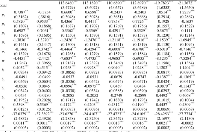
For example, the own price-response of durum
wheat (the p1 row in Table 1) is significant only in the
one-way FE and RE models and in the two-way SUR system, while in other models is not statistically significant. Moreover, among significant parameters, we observe quite a strong variability, since the two-way SUR system estimates a parameter that is approximately 50% higher than those estimated with single equation techniques. The same happens for the other key parameter of the own area payment effect
(the b1 row in the same table). Here all models provide
positive and significant parameters, but their absolute value is strongly different among models. Nevertheless the two-way SUR provides the highest value.
In Table 2 we can appreciate how the SUR technique allows the cross equations restrictions
ji
ij α
α = and γij=γji.
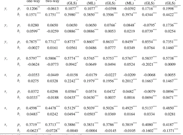
In Table 3 we provide own-price and own-payment elasticities for both the supply and land allocation equations of our model, the key parameters that are used for policy simulations. Once again, results turn out to be quite different across models. For example, limiting our attention to those elasticities significantly different from 0, we have that the own payment
elasticity for oilseeds supply (rows y3 in the table) and
the own price elasticity for maize land allocation (row
s2 in table) are much higher in the case of the two-way
SUR system as compared to all the other models.
VI. CONCLUDING REMARKS
In recent years, a number of agricultural economics papers have been published drawing relevant policy implications from the estimation of arable crop supply/acreage equations carried out on farm-level data.
7
In Tables 1, 2 and 3 we adopt the following convention: y = output supply, p = output price, x = input demand, w = input price, s = land allocation, b = area payment, 1 = Durum wheat, 2 = Maize, 3 = Oilseeds, 4 = Other Cereals, 5 = Other output, sT = total land, c = set-aside percentage and
z = quasi-fixed input (aggregate of capital and family labour).
However, these papers have often adopted a simplified approach in taking into account the complex econometric issues implied by the use of these data, which are typically unbalanced panels. In fact, the use of these data implies the adoption of proper panel-data techniques, which have been recently developed in the econometric literature and that have still to be incorporated as automatic commands in the standard econometric softwares.
In light of these considerations, the present paper re-examines the analyses proposed for Italy by Moro and Sckokai (1999), adopting a more suitable econometric approach. Thus, we model the CAP arable crop regime using FADN data for Italy in order to analyse supply and acreage response to policy parameters. Our empirical application has mainly illustrative purposes, since the main objective of the paper is to underline the different results obtained adopting different panel data techniques.
In terms of econometric approach, the paper relies on the Error Component Model, both in its one-way version (i.e. considering only the individual specific effect) and in its two-way version (i.e. considering both the individual and the time specific effects). Since the estimated model is a set of simultaneous
equations, the corresponding regressions have been estimated both as single equations and as a SUR system of equations. In adopting this last technique, we have extended the one-way SUR technique proposed by Bjorn (2004) to the two-way case.
The preliminary results of our work confirm our initial expectations, since the adoption of different estimation techniques implies obtaining quite different results, both in terms of absolute value of the estimated parameters and in terms of their statistical significance. This seems to suggest that the adoption of proper panel-data techniques is likely to be very important in order to obtain reliable estimates of some key policy parameters, like the output price and area payment elasticities estimated in our model.
However, in this research a further step is needed, since at this stage we are not able to select, through an appropriate test, among our alternative econometric specifications. In fact, as noted by Wooldridge (2001), in presence of heteroscedasticity the standard Hausman test does not perform correctly. Since heteroscedasticity is very common in farm-level data, and it is present also in our sample, our two-way estimators must be modified in order to account for heteroscedastic error terms.
Table 1 Durum wheat supply estimated parameters under different panel-data techniques FE one-way FE two-way RE one-way (GLS) RE one-way (ML) RE two-way (GLS) RE two-way (ML) SURWB two-way (GLS) SUR QUE two-way (GLS) cons 113.6480*** (3.4729) 113.1820*** (3.6027) 110.6890*** (4.0557) 112.8970*** (3.6489) -19.7823*** (1.6353) -21.3672*** (1.5650) 1 p 0.7387 ** (0.3162) -0.3754 (.3816) 0.6600** (0.3048) 0.6598** (0.3078) -0.2437 (0.3651) -0.2403 (0.3668) 1.0514*** (0.2914) 1.2239*** (0.2867) 2 p 0.5820 *** (0.1807) 0.9533*** (0.1868) 0.4366** (0.1687) 0.4411** (0.1707) 0.7858*** (0.1769) 0.7726*** (0.1756) 0.1928 (0.1557) -0.1637 (0.1522) 3 p -0.6987*** (0.1676) -0.7061*** (0.1685) -0.3362** (0.1550) -0.3569** (0.1570) -0.4291*** (0.1591) -0.3529** (0.1573) -0.3675*** (0.1230) 0.1111 (0.1214) 4 p -1.3836*** (0.1441) -1.3270*** (0.1447) -1.2426*** (0.1300) -1.2476*** (0.1318) -1.2118*** (0.1341) -1.1916*** (0.1319) -1.1539*** (0.1130) -1.6945*** (0.1094) 5 p -0.1466 (0.1329) -0.3742** (0.1678) -0.4464*** (0.1265) -0.4294*** (0.1279) -0.6008*** (0.1579) -0.6780*** (0.1584) -0.6019*** (0.1184) -0.7146*** (0.1156) w -4.4451*** (1.267) -2.4421* (1.3965) -7.6837*** (1.2187) -7.4735*** (1.2322) -4.9683*** (1.3469) -5.6935*** (1.3493) -8.1235*** (1.1586) -7.5284*** (1.1354) 1 b 0.4052 *** (0.0934) 0.4515*** (0.0942) 1.0263*** (0 .0856) 0.9928*** (0.0872) 0.9040*** (0.0883) 1.0248*** (0.0875) 1.1202*** (0.0817) 1.1404*** (0.0800) 2 b -0.0491 (0.0569) -0.0499 (0.0604) -0.0537 (0 .0536) -0.0531 (0.0542) -0.0679 (0.0574) -0.0747 (0.0571) -0.1387*** (0.0424) -0.1365*** (0.0419) 3 b -0.0536 (0.0342) 0.0845 (0.0402) -0.0996*** (0 .0330) -0.0975*** (0.0334) 0.0459 (0.0385) 0.0434 (0.0390) -0.0879*** (0.0293) -0.1143*** (0.0290) 4 b 0.0434 (0.1952) -0.0280 (0.2028) -0.2085 (0.1717) -0.2052 (0.1742) -0.2749 (0.1830) -0.2899 (0.1793) 0.4492*** (0.1015) 0.4068*** (0.1004) T s 0.5398 *** (0.0125) 0.5369*** (0.0125) 0.4174*** (0.0073) 0.4203*** (0.0076) 0.4312*** (0.0081) 0.4190*** (0.0076) 0.4457*** (0.0069) 0.4309*** (0.0068) c -37.0379*** (2.4832) -37.3892*** (2.4926) -23.6270*** (2.2858) -24.4107*** (2.3250) -27.4723*** (2.3467) -24.6105*** (2.3273) -28.4253*** (2.1697) -27.7734*** (2.1130) z 0.0011 *** (0.0003) 0.0011*** (0.0003) 0.0017*** (0.0002) 0.0016*** (0.0002) 0.0013*** (0.0003) 0.0016*** (0.0002) 0.0021*** (0.0002) -0.0002 (0.0002) Standard errors in brackets. *** 1% significance, **5% significance, *10% significance
Table 2 Estimated parameters under two-way SUR QUE (GLS) Dependent Variables 1 y y2 y3 y4 y5 w s1 s2 s3 s4 cons -21.3672*** (1.5650) -41.8531*** (4.5059) 22.3254*** (5.3982) -53.5738 (0) -363.5020*** (38.2655) -19.1745*** (2.7951) 4.81388*** (0.1986) -0.1441 (0.1317) 0.3524*** (0.0967) 0.5997*** (0.1563) 1 p 1.2239*** (0.2866) -1.0193 (0.7681) 0.0110 (0.0543) -0.0116 (0 .0204) (0.0301) -0.0359 -0.2858 (0) 2 p -0.1637 (0.1522) 1.6954*** (.3906) 0.7794* (0.4575) -0.0451 (0.0317) 0 .0854*** (0.0200) -0.0678*** (0 .0207) 0.0644 *** (0.0155) 3 p 0.1111 (0.1214) -0.9397*** (0.1240) 5.3231*** (0.1023) 0.5690 (0.3724) -0.1364*** (0.0240) -0.1588*** (0.0109) 1.3750*** (0.0184) -0.1840 (0) 4 p -1.6945*** (0.1094) 0.4467*** (0.1549) -1.5350*** (0.0781) 5.4384*** (0.1317) 1.4904*** (0.3311) -0.3613*** (0.0223) -0.0685*** (0.0104) -0.2250*** (0.0145) 0.8912*** (0.0133) 5 p -0.7146*** (0.1156) 0.5256** (0.2488) -0.2004** (0.0936) -0.0158 (0.1242) -3.1651*** (1.0924) 0.0277 (0.3308) -0.0705*** (0.0222) 0.0001 (0.0138) -0.0178 (0.0158) 0 .0428*** (0 .0150) w -7.5284*** (1.1354) -3.9609** (1.9462) 2.0045*** (0.7617) -1.9126* (0.9835) 0.2082 (6.8105) -5.9019* (3.2356) -0.0731 (0.2236) 0.0568 (0.1183) 0.2691** (0.1308) 0.0634*** (0.0112) 1 b 1.1404*** (0.0800) 1.3579*** (0.1699) -0.1391*** (0.0467) 0.1322 (0.0876) 2.8923*** (0.7058) 0.0676 (0.2317) 0.1233*** (0.0165) 2 b -0.1365*** (0.0419) 0.1276 (0.1411) -0.0816** (0.0331) -0.1496*** (0.0515) -1.4348*** (0.4673) 0.0334 (0.1475) -0.0018 (0.0074) 0.0231*** (0.0067) 3 b -0.1143*** (0.0290) 0.1124 (0.0712) 0.0788*** (0.0272) 0.0353 (0.0330) 0.3742 (0.3027) -0.1765** (0.0882) -0.0303*** (0.0054) -0.0012 (0.0036) 0.0059 (0.0043) 4 b 0.4068*** (0.1004) -2.8680*** (0.2481) 0.3155*** (0.0658) 0.0027 (0.1524) 2.7314*** (0.9696) -1.9420*** (0.3752) 0.0073 (0.0103) -0.0043 (0.0061) -0.0008 (0.0040) -0.0932*** (0.0177) T s 0.4309*** (0.0068) 0.3151*** (0 .0146) 0.2189*** (0.0034) 0.4903*** (0.0088) 2.8609*** (0.0385) -1.8111*** (0.0197) 0.0896*** (0.0013) 0.0373*** (0.0009) 0.0550*** (0.0008) 0.0646*** (0.0010) c -27.7734*** (2.1130) 37.0367*** (5.1371) -7.5390*** (1.7587) -7.0541*** (2.3491) -59.9017*** (19.4647) 46.2878*** (6.0859) -8.0540*** (0.4262) 1.3302*** (0.2800) -1.9134*** (0.2974) -1.0590*** (0.2889) z -0.0002 (0.0002) 0.0181*** (0.0005) -0.0026*** (0.0001) -0.0010*** (0.0002) 0.0178*** (0.0017) -0.0216 (0.0006) 0.0001*** (0.00004) 0.0009*** (0.00003) -0.0003*** (0.00002) -0.0001** (0.00003) Standard errors in brackets. *** 1% significance, **5% significance, *10% significance
Table 3 Estimated own-price and own-payment elasticities under different panel-data techniques FE one-way FE two-way RE one-way (GLS) RE one-way (ML) RE two-way (GLS) RE two-way (ML) SURWB two-way (GLS) SUR QUE two-way (GLS) 1 y p1 0.1206** -0.0613 0.1077** 0.1077** -0.0398 -0.0392 0.1716*** 0.1998*** 1 b 0.1571*** 0.1751*** 0.3980*** 0.3850*** 0.3506*** 0.3974*** 0.4344*** 0.4422*** 2 y p2 0.0280 0.0650 0.0650 0.0650 0.0766 * 0.0848* -0.0795* 0.1736*** 2 b 0.0599** -0.0259 0.0886*** 0.0886*** 0.0053 0.0219 0.0739*** 0.0254 3 y p3 0.7875 *** 0.7712*** 0.8775*** 0.8607*** 0.8633*** 0.8459*** 0.8554*** 0.7351*** 3 b -0.0027 0.0161 0.0561 0.0486 0.0777 0.0349 0.0764 0.1460*** 4 y p4 0.5797*** 0.5806*** 0.5774*** 0.5765*** 0.5753*** 0.5767*** 0.5837*** 0.5738*** 4 b -0.0624 -0.0773 0.0942* 0.0649 0.0494 0.0524 -0.2021*** 0.0009 1 s p1 -0.0353 -0.0449 -0.0158 -0.0179 -0.0227 -0.0209 -0.0068 0.0055 1 b 0.0275 0.0328 0.2242*** 0.1979*** 0.1956*** 0.2012*** 0.1663*** 0.1467*** 2 s p2 0.0372 0.0298 0.0584** 0.0574 0.0472* 0.0482** -0.0079 0.0896*** 2 b 0.0333** -0.0188 0.0435*** 0.0430*** 0.0037 0.0016 0.0694*** 0.0471*** 3 s p3 0.4598 *** 0.4478*** 0.5129*** 0.5039*** 0.5026*** 0.4925*** 0.5137*** 0.4850*** 3 b 0.0483** 0.0242 0.0494*** 0.0503** 0.0369 0.0164 0.0334 0.0281 4 s p4 0.3719 *** 0.3713*** 0.3886*** 0.3831*** 0.3786*** 0.3819*** 0.4080*** 0.4187*** 4 b -0.0623** -0.0728** -0.0040 -0.0004 -0.0145 -0.0105 -0.1602*** -0.1371*** *** 1% significance, **5% significance, *10% significance
REFERENCES
1. Baltagi B H (2005) Econometric analysis of panel data (3rd edition). Wiley and Sons, Chichester
2. Baltagi B H, Bresson G, Pirotte A (2005) Adaptive estimation of heteroskedastic error component models. Econometric Reviews 24: 39-58
3. Baltagi B H, Song S H, Jung B C (2001) The unbalanced nested error component regression model. Journal of Econometrics 1061: 357-381
4. Biørn E (2004) Regression systems for unbalanced panel data: a stepwise maximum likelihood procedure. Journal of Econometrics 122: 281-291
5. Boumahdi R, Chaaban J, Thomas A (2004) Import demand estimation with country and products effects: application of multi-way unbalanced panel data models to Lebanese imports. Cahier de Recherche INRA de Toulouse 2004-17
6. Chavas J P, Holt M T (1990) Acreage decision under risk: the case of corn and soybeans. American Journal of Agricultural Economics 72: 529-538
7. Davis P (2002) Estimating multi-way error components models with unbalanced data structures. Journal of Econometrics 106: 67-95
8. Goodwin B K, Mishra A K (2006) Are ‘decoupled’ farm program payments really decoupled? An empirical evaluation. American Journal of Agricultural Economics 88: 73-89
9. Greene W (2003) Econometric analysis (5th edition). Prentice Hall, New York
10. Hausman J A (1978) Specification tests in Econometrics. Econometrica 46: 1251-1271
11. Li Q, Stengos T (1994) Adaptive estimation in the panel data error component model with heteroskedasticity of unknown form. International Economic Review 35: 981-1000
12. Mazodier P, Trognon (1978) Heteroskedasticity and stratification in error components models. Annales de l’Insee 30-31: 451-482
13. Moro D, Sckokai P (1999) Modelling the CAP arable crop regime in Italy: degree of decoupling and impact of Agenda 2000. Cahiers d’Economie et Sociologie Rurales 53: 49-73
14. Oude Lansink A, Peerlings J (1996) Modelling the new EU cereals regime in the Netherlands. European Review of Agricultural Economics 23: 161-178
15. Oude Lansink A (1999) Area allocation under price uncertainty on Dutch arable farms. Journal of Agricultural Economics 50: 93-105
16. Randolph W C (1988) A transformation for heteroscedastic error components regression models. Economic Letters 27: 349-354
17. Roy N (2002) Is adaptive estimation for panel model with heteroskedasticity in the individual specific error component? Some Monte Carlo evidence. Econometric Reviews 21: 189-203
18. Sckokai P, Anton J (2005) The degree of decoupling of area payments for arable crops in the European Union. American Journal of Agricultural Economics 87: 1220-1228
19. Sckokai P, Moro D (2006) Modeling the reforms of the Common Agricultural Policy for arable crops under uncertainty. American Journal of Agricultural Economics 88: 43-56
20. Serra T, Zilberman D, Goodwin B K, Featherstone A (2006) Effects of decoupling on the mean and variability of output. European Review of Agricultural Economics 33: 269-288
21. Serra T, Zilberman D, Goodwin B K, Hyvonen K (2005) Replacement of agricultural price supports with area payments in the European Union and the effects on pesticide use. American Journal of Agricultural Economics 87: 870-884
22. Shonkwiler J S, Yen S T (1999) Two-step estimation of a censored system of equations. American Journal of Agricultural Economics 81: 972-982
23. Wansbeek T, Kapteyn A (1989) Estimation of the error-components model with incomplete panels. Journal of Econometrics 41: 341-361
24. Wooldridge J M (2001) Econometric analysis of cross section and panel data. The MIT Press, Cambridge
Corresponding author: • Paolo Sckokai
• Istituto di Economia Agro-alimentare Università Cattolica del Sacro Cuore • via Emilia Parmense 84
• 29100 Piacenza • Italy