Improving Efficiency in Deep Learning for Large Scale Visual Recognition

(1)

University of Central Florida University of Central Florida

STARS

Electronic Theses and Dissertations, 2004-2019

2016

Improving Efficiency in Deep Learning for Large Scale Visual

Recognition

Baoyuan Liu

University of Central Florida

Part of the Computer Engineering Commons

Find similar works at: https://stars.library.ucf.edu/etd University of Central Florida Libraries http://library.ucf.edu

This Doctoral Dissertation (Open Access) is brought to you for free and open access by STARS. It has been accepted for inclusion in Electronic Theses and Dissertations, 2004-2019 by an authorized administrator of STARS. For more information, please contact [email protected].

STARS Citation STARS Citation

Liu, Baoyuan, "Improving Efficiency in Deep Learning for Large Scale Visual Recognition" (2016). Electronic Theses and Dissertations, 2004-2019. 5317.

(2)

IMPROVING EFFICIENCY IN DEEP LEARNING FOR LARGE SCALE VISUAL RECOGNITION

by

BAOYUAN LIU

B.S. Shanghai Jiao Tong University, 2010 M.S. University of Central Florida, 2013

A dissertation submitted in partial fulfilment of the requirements for the degree of Doctor of Philosophy

in the Department of Electrical Engineering and Computer Science in the College of Engineering and Computer Science

at the University of Central Florida Orlando, Florida

Fall Term 2016

(3)

c

(4)

ABSTRACT

The emerging recent large scale visual recognition methods, and in particular the deep Convolu-tional Neural Networks (CNN), are promising to revolutionize many computer vision based artifi-cial intelligent applications, such as autonomous driving and online image retrieval systems. One of the main challenges in large scale visual recognition is the complexity of the corresponding algorithms. This is further exacerbated by the fact that in most real-world scenarios they need to run in real time and on platforms that have limited computational resources. This dissertation focuses on improving the efficiency of such large scale visual recognition algorithms from several perspectives.

First, to reduce the complexity of large scale classification to sub-linear with the number of classes, a probabilistic label tree framework is proposed. A test sample is classified by traversing the label tree from the root node. Each node in the tree is associated with a probabilistic estimation of all the labels. The tree is learned recursively with iterative maximum likelihood optimization. Comparing to the hard label partition proposed previously, the probabilistic framework performs classification more accurately with similar efficiency.

Second, we explore the redundancy of parameters in Convolutional Neural Networks (CNN) and employ sparse decomposition to significantly reduce both the amount of parameters and compu-tational complexity. Both inter-channel and inner-channel redundancy is exploit to achieve more than 90% sparsity with approximately 1% drop of classification accuracy. We also propose a CPU based efficient sparse matrix multiplication algorithm to reduce the actual running time of CNN models with sparse convolutional kernels.

Third, we propose a multi-stage framework based on CNN to achieve better efficiency than a single traditional CNN model. With a combination of cascade model and the label tree framework, the

(5)

proposed method divides the input images in both the image space and the label space, and pro-cesses each image with CNN models that are most suitable and efficient. The average complexity of the framework is significantly reduced, while the overall accuracy remains the same as in the single complex model.

(6)

ACKNOWLEDGMENTS

I would like to thank my advisor, Dr. Hassan Foroosh, for his guidance, encouragement and pa-tience. He has been always supportive with me and given me numerous great advices on research. Discussing research with him has always been enlightening and also fun. I’m deeply honored to be his PhD student.

I would also like to thank Dr. Marshall Tappen, who has been my advisor for one year in UCF and my manager while I was an intern in Amazon. Joining his group was the turning point of my Phd career and the best decision I’ve made these years. I cannot imagine how he can treat me more generously . I’ve learned so much from him both on research and on life.

This thesis is not possible without the love and support from my wife, Min Wang. The years that we spent together at UCF has been the best years in my life. Both research and life become much more delightful with her companion. We have been through all the happiness and sorrow together, and every detail in this Phd with her would be the best things to remember for my whole life.

Finally, I’m extremely grateful to my parents. Whenever I felt depressed, the weekly chat with them on Friday night always brought me hope and cheered me up. Every time I went back to China and stayed with them for a month, I became totally revived. This journey would be much harder without their unconditional support and sacrifice.

(7)

LIST OF FIGURES

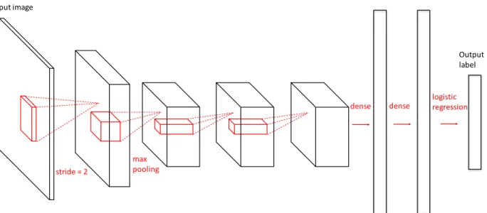
1.1 An example Convolutional Neural Network (CNN). The input of CNN is a color image and the its output is the probability of each label. The essential building block of CNN is the convolutional layer. . . 5

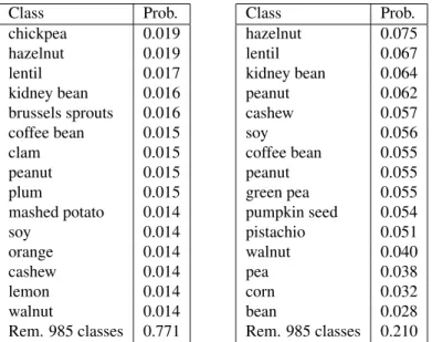
3.1 This figure visualizes the expansion process for one part of the tree. The table in (a) shows a portion of the categorical distribution at a branch node in the second level of a T6,4 tree that has four levels, excluding the root node. The tables in (b), (c), and (d) show the categorical distributions learned for three of the child nodes. The probability in these child nodes is more concentrated on a subset of the classes than in the parent node. In this result, the tree has not been trained with the pruning techniques in Section.3.5.1, so the distributions accurately represent the behavior of the maximum-likelihood criterion. . . 27

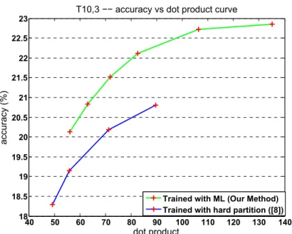
3.2 Accuracy vs dot product curve for our T10,3 tree. The green curve shows our method using maximum likelihood with multinomial estimation. The blue curve shows the result using hard label partition[16] with our framework. The maximum likelihood method achieves consistent higher classification accuracy with similar average dot products needed at test time . . . 36

3.3 Accuracy vs dot product curve for our T6,4 tree. Again, the tree trained with the maximum likelihood approach has consistently higher accuracy. . . 36

(13)

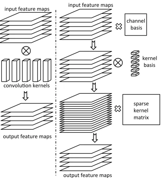
4.1 Overview of our sparse convolutional neural network. Left: the operation of convolution layer for classical CNN, which convolves large amount of con-volutional kernels with the input feature maps. Right: our proposed SCNN model. We apply two-stage decompositions over the channels and the convo-lutional kernels, obtaining a remarkably(more than 90%) sparse kernel matrix and converting the operation of convolutional layer to spare matrix multipli-cation. . . 40

4.2 Matrix Multiplication Algorithm in OpenBLAS. The input matrices are first divided into blocks which can fit in L2 cache. Each block is then divided into 8 element wide strips. The multiplication outputs of two strips are held in 8 AVX registers during calculation. . . 45

4.3 An example that illustrates how our algorithm generates code for multiplying a dense matrix and a sparse matrix . . . 47

4.4 Comparison of initial decomposition methods. We show the variation of both the accuracy and the average sparsity of our sparse CNN during the training process. . . 52

4.5 Average ratio of non-zero elements in our sparse convolution kernels corre-sponding to the bases of decompositions over channels and filters. (a) (b) show the bases over channels and (c) to (g) show the bases over filters.The bases in each figure are sorted in descending order of their eigenvalues in PCA initialization. . . 53

(14)

4.6 Comparison between the original convolution kernels and the convolution kernels reconstructed from our sparse kernels. Here we show randomly sam-pled kernels conv1, conv2 and conv3 layers. conv4 and conv5 are very sim-ilar to conv3. For each layer, the first row shows the original kernels and the second row shows the reconstructed ones. The average cosine similarity between them are displayed under. . . 54

4.7 Running time analysis of our sparse-dense matrix multiplication algorithm. The horizontal axis stands for the percentage of non-zero elements in the input sparse matrix, and the vertical axis is the relative running time com-paring to the dense matrix multiplication code in OpenBLAS. The arithmetic time is the running time of multiplication and addition, and the I/O time in-cludes loading the input matrix from memory to cache, loading from cache to CPU and writing result to memory. The theoretical time is the best possible speedup one can achieve, which is identical to the density of the input matrix. 55

5.1 The probability of one class confusing with other classes. The shown class is relatively heavily confused with a few classes, while slightly confused with a large number of classes. This “long tail” property of confusion leads us to the idea of cascading label tree model. . . 62

5.2 Flow chart of our multi-stage framework. All the input images are processed by the first stage. The stage predictor determines whether to directly output label predicted by first stage, or assign the image to the label tree model in 2nd or 3rd stage for more accurate prediction. The 3rd stage label tree model has heavier label overlapping, and is more accurate and complex than 2nd stage. . . 65

(15)

5.3 Relationship between the ambiguity and accuracy for label clustering algo-rithm with different number of clusters . . . 73

5.4 Comparison of accuracies between fine-tuning separate CNN models for each cluster and using one single CNN model for all the categories, assuming that the 1st stage is optimal. For both 2nd and 3rd stage, all the clusters show significant improvement. . . 74

5.5 Overall accuracy as a function of the ratio of selecting 1st stage model and 2nd stage model by the stage predictor. When the ratios of 1st stage and 2nd stage are approximately less than 35%, the accuracy decreases very slowly. . 75

5.6 Comparison of our framework with other classical CNN models and our 2nd and 3rd stage model. Our framework achieves significant improvement on accuracy/complexity ratio over single CNN models. . . 76

(16)

LIST OF TABLES

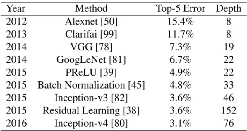
2.1 Performance of Recent Deep CNN models. . . 13

3.1 Comparison of our method and [16] with different tree configuration on ILSVRC 2010 dataset.T m, ndenotes the tree that hasmchildren per node when

branch-ing andnlevels. We show the classification accuracy(Acc) and the test time

speedup Ste. The first row shows the result using our ML based method.

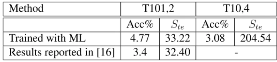
The second row is the result using hard label partition and our probabilistic framework as explained in Section 3.6.2. Our method significantly outper-forms [16]. The accuracy of maximum likelihood (ML) is consistently better than the hard label partition with similar speedup. For reference, the last row shows the accuracy produced by a multi-class SVM trained with LIBLIN-EAR. . . 32

3.2 Result on Imagenet 10K. While the accuracy numbers cannot be compared directly because of differences in the test set(see text), these results show that our method can scale to large numbers of classes and performs reasonably. . 33

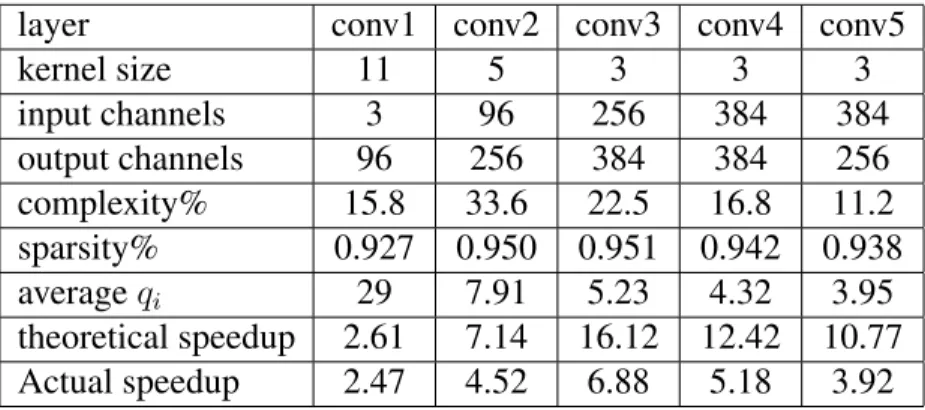
4.1 Sparsity, Average number of bases ,theoretical and actual speedup corre-sponding to each convolutional layer for our SCNN model. q_i is the average

number of bases in each channel. Results demonstrates that our highly sparse model could lead to remarkably acceleration for computation in both theory and practice. . . 50

(17)

4.2 Comparison between a model, similar to [40], trained with sparsity and the speedup factors reported in [18]. . . 51

4.3 Running time analysis and comparison with original dense networks. All the numbers for each layer are normalized with the layer’s total running time with our method. The last row is the speed-up factor of our method. . . 56

4.4 Mean average precision of object detection with our method compared with [40]. “bb” stands for bounding box regression, “1s” means 1 scale and “5s” means 5 scales. Our sparse model is inferior to [40] by approximately 2%. . . 57

5.1 Configuration of the CNN models used in our framework. They vary in in-put size, number of convolutional layers, resulting in diverse complexity and accuracy. . . 70

5.2 Configuration of 1st stage model . . . 71

(18)

CHAPTER 1: INTRODUCTION

Visual recognition analyzes the information from an image and recognizes the type of objects in it. Visual recognition with sufficient accuracy and reliability is essential for a successful artificial intelligence system. For smart AI systems, such as autonomous driving, home assistant robot, and online image retrieval systems, the ability to recognize the visual objects is preliminary of performing more advanced intelligent behaviors.

Researchers have been working on the problem of visual recognition for decades. Due to limited resource of images and computing power, the visual recognition systems in the early days were trained and evaluated on small scale datasets, which typically include a few hundreds of categories and each category contains less than one hundred images. In recent years, with the dramatically increase of internet images and computing resources, training large scale systems that attempt to match human’s intelligence becomes practical and attracts more and more attention.

The problem of large scale visual recognition is challenging for computers. First, the visual world is an extremely complicated space that is determined by many underlying physical factors. For objects within the same category, viewpoint, distance, illumination condition, occlusion, and back-ground clutters can all effectively modify each pixel of its image. Second, the number of categories are naturally large for human vision system. Humans are able to recognize approximately 30 thou-sand different categories. An AI system that is designed to function as well as human, such as an autonomous driving agent, is required to possess comparable recognition ability. Third, many categories are easy to confuse with each other, which poses another level of challenge.

The difficulty of large scale visual recognition leads to the complexity of corresponding algorithms. Due to the complicated image space and the heavy confusion between similar categories, large amount of complex operations are necessary to transfer the images to a more separable space

(19)

in which machine learning algorithm can be utilized to train an effective classifier; In addition, the large number of categories also increases the complexity of the classifier, since each category requires certain amount of parameters to represent its distribution in the transformed feature space.

On the other hand, in most real world scenarios, the visual recognition systems are required to run with near real-time processing speed, but at platforms that possess limited amount of computing resource. For instance, in a home assistant robot or an auto-piloting drone, the AI systems need to response in typically less than 100ms to make sure it can work smoothly and handle emergency quickly. In contrast, due to limited space and battery life, the systems are most likely running on embedded System on Chip platforms, which have very limited computing power comparing to the servers and GPUs that are currently used to train large scale image classification models.

Therefore, the efficiency of current large scale recognition algorithms becomes a prohibiting bot-tleneck that limits their wider adoptions in many potential applications. In this dissertation, I focus on improving the efficiency of large scale visual recognition algorithms.

A standard pipeline of traditional image classification algorithm involves two fundamental stages. In the first stage, information is extracted from the raw pixels of each image, and is represented by a 1D feature vector. This stage is traditionally called feature extraction. A desirable feature extraction algorithm describes the categorical characteristics from the images, while is invariant to in-class diversity. In the second stage, a multi-class statistical classifier is trained and evaluated based on the generated feature vectors.

The computational complexity of an image classification system is the sum of these two stages. The feature extraction is performed once for each image regardless of the number of categories, while the complexity of the classifier is highly dependent on the scale of the problem. Therefore, when the size of the dataset scales up, the complexity of the classifier becomes the bottleneck of the whole framework.

(20)

For large scale problems, since both the number of images and the number of categories increase dramatically, the classifier should be chosen so that the complexity of both training and inference is limited to acceptable level. Linear 1-vs-all SVM or multi-class logistic regression model achieves similar inference complexity, which is linear to the length of feature vector and number of classes. The parameters for the popular linear SVM and multinomial logistic regression models contain one vector per possible class. Thus, if there areK possible classes, assigning a label to a new feature

vectorxwill require the computation of K dot products between xand the vectors defining the

classifier. For a relatively small number of categories, this computational cost is not significant enough to require attention.

However, as both the number of categories and need for fast recognition increases, this linear relationship between the complexity of recognition and the number of classes can become prob-lematic. This issue is compounded if the classification process involves computations that are more complex than a dot product.

In [6], Bengio et al. introduce the label tree model for reducing the complexity of recognition in a problem with a larger number of classes. In the label tree model, a feature vector is assigned a label by traversing a tree. At each node visited, the classifier computes the dot product between the feature vector and a small number of vectors. This tree structure causes the classification complexity to grow logarithmically, rather than linearly, with the number of classes.

In Chapter 3, we present a novel, probabilistic approach to learning the parameters of a label tree. We show how a recursive process learns the tree parameters. The probabilistic approach provides a natural way of soft label partitioning, and is able to pass the label distribution as a prior information down to the leaf nodes. As the results in Section 3.6 will show, this approach produces significantly improved accuracies over previous results in [16]. The probabilistic model also makes it possible to tune accuracy versus efficiency without having to retrain the tree.

(21)

From a broader perspective, formulating the label tree in a probabilistic framework provides a straight-forward avenue for integrating more complex, accurate classification models into the label tree framework. With this probabilistic formulation, any classifier that can be expressed proba-bilistically can be integrated into the label tree.

In 2012, Krizhevsky et. al. [50] first propose to use Convolutional Neural Networks (CNN) to solve the large scale image classification problem, and significantly improves the state-of-the-art on ImageNet LSVRC [14] dataset, which includes one thousand categories and 1.2 million training images. Since then, the research of visual recognition has come to the deep learning era. Numerous improvement have been made on CNN, with the depth of the network increasing from 7 to hundreds, and the top-5 error on ImageNet LSVRC dataset reduced from 16% to as low as 3.5%.

CNN is a type of feed-forward artificial neural network that is specifically designed to recognize image signal. In CNN, the connections between neurons are organized in a convolutional fashion, so that each neuron receives information from a small local receptive field rather than all the bottom neurons. As in standard neural network, a non-linear neuron function is performed on the output of each neuron, making the network able to learn highly complex distributions in feature space. Spatial pooling layers are also occasionally used to reduce the spatial dimension of feature and gather information. At the end of CNN, a multi-class classifier, most commonly logistic regression, maps the transformed feature space to the space of semantic categories. Figure. 1.1 shows an example CNN model. In general, the spatial dimension of the feature map is gradually reduced by pooling or convolution with stride, while the number of channels increases with the depth of the network.

Due to the complexity of image space, large amount of convolutional layers are required to transfer the images into separable space. However, convolutional layers are computationally expensive.

(22)

Input image Output label logistic regression dense max pooling stride = 2 dense

Figure 1.1:An example Convolutional Neural Network (CNN). The input of CNN is a color image and the its output is the probability of each label. The essential building block of CNN is the convolutional layer.

Each convolutional kernels involves convolving with all the input channels. and the number of input and output channels need to be large to retain the information in the image. Results of ImageNet LSVRC competitions in recent years have demonstrated a strong correlation between the network size and the classification accuracy. The ILSVRC 2014 submission from VGG [77] builds a network with up to 16 convolutional layers that reduces the top-5 classification error to 7.4%, at the expense of approximately one month of network training with 4 high-end GPUs.

The structure of CNNs makes it reasonable to conjecture that there exists heavy redundancy in these networks. Due to the highly non-convex property of neural networks, over-parameterization with random initialization is necessary to overcome the negative impact of local minimum in net-work training. Additionally, the fact that no independence constraint is imposed among the convo-lutional kernels for each layer in the training phase also indicates high potential for redundancy.

In Chapter 4, we show that this redundancy makes it possible to notably reduce the amount of computation required to process images, by sparse decomposition of the convolutional kernels. As

(23)

Figure 4.1 illustrate, two-stage decomposition’s are applied to explore the inter-channel and intra-channel redundancy of convolution kernels. We first perform an initial decomposition based on the reconstruction error of kernel weights, then fine-tune the network while imposing the sparsity constraint. In the fine-tuning phase, we optimize the network training error, the sparsity of con-volutional kernels, as well as the number of concon-volutional bases simultaneously, by minimizing a sparse group-lasso object function. Surprisingly high sparsity can be achieved in our model. We are able to zero out more than 90% of the convolutional kernel parameters of the network in [51] with relatively small number of bases while keeping the drop of accuracy to less than 1%.

In our Sparse Convolutional Neural Networks (SCNN) model, each sparse convolutional layer can be performed with a few convolution kernels followed by a sparse matrix multiplication. It could be assumed that the sparse matrix formulation naturally leads to highly efficient computation. How-ever, computing sparse matrix multiplication can involve severe overhead that makes it difficult to actually achieve attractive acceleration. Thus, we also propose an efficient sparse matrix multipli-cation algorithm. Based on the fact that the sparse convolutional kernels are fixed after training, we avoid the necessity of indirect and discontinuous memory access by encoding the structure of the input sparse matrix into our program as the index of registers. Our CPU-based implementation demonstrates much higher efficiency than off-the-shelf sparse matrix libraries and a significant speedup over the original dense networks is realized. While convolutional network systems are dominated by GPU-based approaches, advances in CPU-based systems are useful because they can be deployed in commodity clusters that do not have specialized GPU nodes.

While the idea of label tree is able to significantly reduce the complexity of large scale multi-class classifier, it will make very little improvement of efficiency on the CNN framework. Different from the Bag of Visual Words (BoVW) model, most of the computation is consumed by the con-volutional layers in CNN, which can be considered as a form of feature extractor, and need to be performed for images from all categories. The complexity of the convolutional layers is highly

(24)

dependent on the difficulty of the problems, namely, the number of categories and the level of confusion between them. When the number of categories is small and they are easy to distinguish, only a few number of convolutional layers are adequate separate them in feature space; While for more complicated dataset, a deeper stack of convolutional layers are necessary to achieve accuracy classification. Therefore, reducing the the original large scale problem to smaller scale, less com-plex problem will lead to a decrease of the comcom-plexity of convolutional layers, thus increasing the efficiency of the overall CNN framework.

In Chapter 5, we propose to decompose a single CNN model of high complexity into a multi-stage, tree structured framework of multiple efficient models. Instead of processing each image with a single computationally expensive network, coarse probabilistic estimates of the level of “difficulty” of the images are first estimated, and then assigned to models that are trained to recognize specific categories, with different levels of complexity. In this way, we trade the amount of memory space for less run time. The proposed framework is built on the idea of combining the cascade model [88] and the label tree algorithm [7].

(25)

CHAPTER 2: LITERATURE REVIEW

2.1 Image Classification

Bag of Visual Words (BoVW) framework has been the standard pipeline for image classification before CNN. For each input image, large amount of distinctive local patches are detected, and then represented with descriptors with certain types of invariance, such as SIFT [62] and LBP [93]. The descriptors for the whole training dataset are clustered into a “codebook”, and each cluster center is called one “codeword”. Each local patch is assigned to the nearest codeword. For each image, a histogram that describes the frequency of occurrence of each codeword is generated. Then a multi-class classifier is trained based on the histograms.

A few variants have been proposed to improve the performance of BoVW model. Spatial Pyramid Matching (SPM) model [55] provides a framework that takes advantage of the spatial information without sacrificing the robustness and invariance of BoVW.The input image is partitioned into increasing fine sub-regions, and a histogram of visual words are generated in each sub-region. The histograms are weighted and concatenated into one feature vector, which are used for training and predicting with multi-class classifier.

The histograms generated by standard BoVW framework lie in a non-linear high dimension space, and requires linear Mercer kernel SVM to achieve optimal performance. However, for non-linear SVMs, the training complexity is quadratic with number of training samples and the test complexity is linear with number of support vectors. This makes them impractical to be adopted for large scale image categorization problems, in which the number of training images can be as large as millions.

(26)

non-linear kernel SVMs. In [66] and [87], the histograms generated by BoVW are projected to linear space with specifically designed function, so that the kernel distances between the original histogram is approximately equal to the Euclidean distances between the projected feature vectors. Substituted the vector quantization process with sparse coding have been shown in [97] to achieve much better accuracy with linear SVM than the standard vector quantization with non-linear kernel SVM. In [92], Wang et al. propose Locality-constrained Linear Coding (LLC) scheme to further improve the accuracy of feature encoding. In LLC, locality constraint was imposed while encoding each feature, and they were combined in a max pooling fashion to form the feature vector of each image.

In [75], Perronnin et al. propose Fisher Vector representation, which is an alternative way of aggregating the local features to global representation based on the theory of Fisher Kernel [46]. The local features are first modeled with Gaussian Mixture Model (GMM). And each local feature is described by the gradient of its log-likelihood over the means and variances of GMM models. The representation of one image is obtained by aggregating the descriptor of all its local features. In BoVW, the k-means clustering and hard assignment can be considered as a vector quantization procedure, which only describes local distance information. In contrast, the Fisher Vector uses the gradients over parameters to provide much richer and more accurate information. Fisher Vector is shown to significantly outperforms BoVW in several standard datasets.

In [48], Jegou et al. propose Vector of Locally Aggregated Descriptors (VLAD), a simplified, non-probabilistic version of Fisher Vector. In VLAD, the local features are clustered with k-means and hard assigned to their nearest center as in BoVW. Then the difference between each feature and its nearest center is aggregated as the representation of the whole image. This representation can be considered as only describe the gradient over the mean of Fisher Vector model.

(27)

than BoVW. To address this problem, in [76] the Fisher Vector representation is compressed with Product Quantization (PQ) technique. They show that the Fisher Vector can be significantly com-pressed with very little drop of accuracy.

2.2 Label Tree

For a multi-class classification problem with N classes, the inference complexity of traditional

multi-class classifier is at leastO(N). Although the non-linear kernel SVM achieves best accuracy

in general, its complexity is proportional to the number of support vectors for each class, there-fore is not scalable for large scale problems. For linear multi-class SVM, since SVM is a binary classifier, multi-class problems need to be reduced to a series of binary classification problems to which SVM can be directly applied [43][19]. The complexity of multi-class SVM is dependent on the method of reduction. For one-vs-all method, in which a binary classifier is trained for each class against all the other classes, the complexity isO(N); while for one-vs-one method, in which

a binary classifier is trained for each pair of classes, the complexity is O(N2). For multi-class

logistic regression model, which is naturally a multi-class classifier, the complexity is alsoO(N).

To further reduce the inference complexity to sub-linear withN, researchers have been focusing

on building a hierarchical tree structure of classifiers. In the tree structure, each node is associated with a set of classes. The root node includes all the classes. Each class of one node is assigned to one of its children, and a classifier is trained to distinguish the classes of its children nodes. In the traditional “flat” structure such as one-vs-all SVM and multi-class logistic regression model, each binary classifier is only able to distinguish one class, while in hierarchical tree structure, multiple classes can be separated (discarded) with one binary classifier. In this way, the overall complexity can be reduced toO(log(N)).

(28)

The essential challenge of building a hierarchical label tree model is how to learn the structure of the tree recursively, namely, for each node, how many children it should have and how to assign its classes to its children. This problem is equivalent to performing a hierarchical partition-ing/clustering over the classes. In ideal scenario, the classes of one node should be partitioned in a way that the classes inside each child is relatively more confusing and the classes between children are more separable, so that least error is made at this node. However, there is no standard measurement for level of confusion between classes, and the different clustering algorithms can lead to different performance.

One class of methods use the distribution of feature vectors to cluster the categories. In [90] and [60], each class is represented by the mean of the feature vectors of its samples, and the classes are clustered with simple k-means algorithm. In [12], the distance between two classes are measured as the Kullback-Leibler distance [52] between their density functions. A max-cut algorithm is employed to obtain the partition of classes. In [101], a separability measurement based on support vector data description is adopted to represent the distances between classes, and the classes are clustered in a agglomerative fashion. Another class of methods measure the distance between categories by the confusion matrix of classification. In [35] and [7], a confusion matrix is obtained by cross-validation on the training set with traditional one-vs-all SVM, and the classes are partitioned with spectral clustering algorithm [70]. Comparing to feature distribution based clustering, the confusion matrix provides a better description of separability in a discriminative fashion, while at the cost of requiring expensive training with traditional SVM.

The most accurate way of performing the classes partition is to learn the partition and the classifier for each node simultaneously. Since the ultimate goal of partitioning is to reduce the probability of assigning the samples to the wrong child node, minimizing a loss function based on the clas-sification error of node classifier achieves this goal directly. This strategy is adopted in both [16] and [28]. In both work, a max-margin based classifier is learned while the classes in each node are

(29)

optimized as latent variable.

In the hierarchical label tree framework, the number of classes in each node decreases as the tree grows deeper. For the root node, each of its children may contain hundreds of classes, while for the parents of leaf nodes, each of its children only contains one class. This lead to the problem that the nodes close to the root needs to solve more difficult classification problems since the feature distribution is more complex. With a hard partition of classes, the non-separable classes will inevitable suffer mis-classification. To alleviate this problem, a relaxed partition scheme with overlapping is proposed in [68] and also adopted in [28] and [16]. In the relaxation scheme, the classes that are not separable in current node are assigned to all of its children. In this way, the most separation of most confusing classes can be postponed to the deeper nodes, which have much less number of classes in its children. The level of relaxation, namely, the amount of overlapping, controls the balance between accuracy and speed. More overlapping makes the system less easy to make false classification, at the same time increases the number of classes in the children nodes.

The label embedding technique [7][26][2][32] can also be used to reduce the inference complexity from an orthogonal perspective. The original label space is mapped with a linear function to an embedded space, in which the distances between labels are better defined. The label embedding is commonly used to solve the multi-label classification problems. The inference complexity is only proportional to the dimension of the embedded space. Therefore, one can achieve lower complexity when the dimension of the embedded space is lower than the number of labels.

2.3 Convolutional Neural Networks

The famous paper by Krizhevsky et al. in 2012 [50] is a milestone for large scale visual recogni-tion. They are the first one who successfully use deep neural networks to significantly outperform

(30)

the BoVW framework in visual recognition problems. They combined several clever techniques to train a powerful CNN model efficiently. First, they substitute Rectified Linear Unit (ReLU) function for traditional sigmoid function as the non-linear neuron, and significantly improve the network’s converging speed. Second, to avoid overfitting, they adopt two effective strategies: (1) the input images are augmented by random cropping and color jittering; (2) In fully connected layers, the output of the neurons are randomly set to zeros. Third, they implement a GPU-based training framework that is several times more efficient than CPU counterpart.

Following their work, enormous effort has been made to improve the performance and efficiency of CNN [99] [81][78][38] [80] [45][39]. Table 2.1 lists the accuracies of recent deep CNN models and their depth. While the top-5 error rate has been reduced from 15.4% to as low as 3.1% in only a few years, the depth and complexity of the networks are consistently shown to be essential for better performance.

Table 2.1: Performance of Recent Deep CNN models.

Year Method Top-5 Error Depth 2012 Alexnet [50] 15.4% 8 2013 Clarifai [99] 11.7% 8 2014 VGG [78] 7.3% 19 2014 GoogLeNet [81] 6.7% 22 2015 PReLU [39] 4.9% 22 2015 Batch Normalization [45] 4.8% 33 2015 Inception-v3 [82] 3.6% 46 2015 Residual Learning [38] 3.6% 152 2016 Inception-v4 [80] 3.1% 76

The structure of CNN models are highly flexible. The convolutional kernel sizes, the feature map sizes, the number of channels and the number of layers can all be configured. While the structure of Alexnet is just one possible configuration that is limited by the computing resources, researchers have adjusted the configuration of CNN models to achieve better balance of accuracy

(31)

and efficiency. Zeiler et al. [99] propose a visualization technique that shows the function of each intermediate layer, and adjust the kernel size and stride of lower convolutional layers so that they can retain much more useful information. In [58], the fully connected layers are substituted with global average pooling, which significantly reduce the memory required to store the model with almost no loss of accuracy. In [78],3_×3convolutional kernels are exclusively adopted to build a

19 layers network. The network achieves state-of-the-art accuracy in ILSVRC 2014 competition, although the amount of computation is also extremely high. Within the same competition, Szegedy et al. introduce an architecture codenamed “Inception”. In each “Inception” layer, convolutional layers with various kernel size and a max pooling layer are performed on the same input feature map, and the outputs are concatenated. To reduce the amount of computation, the number of input channels is first reduced by a1_×1convolutional layer before fed to convolutional layer with larger

kernel size. With carefully crafted design, their model called GooLeNet achieves better accuracy than [78] with several times less computation. In [38], a bottleneck structure, in which both the input and output channel dimensions of 3 _×3 convolutional layers are reduced, is proposed to

further reduce the computation. In [82], Szegedy et al. use stacked1_×nandn_×1convolutional

layers to replacen_×nconvolutional layers. This adjustment makes it practical to include kernels

as large as1_×7and7_×1with acceptable complexity.

When the depth of CNN models increases, the networks get harder to converge. Initialization plays an important role at the training of deep CNN models. The parameters of each layer are randomly initialized with Gaussian distribution. Too large parameters lead an explosion in the last layer and make the network diverge, while too small parameters will lead to gradient vanishing and make the network converges extremely slow.

To solve this problem, Glorot et al. [31] analyze the behavior of the activation of each layer, and propose a normalized initialization method, so that in the forward pass, the variance of output remains the same as input, while in the backward pass, the variance of the input gradient remains

(32)

the same as the output gradient. He et al. [39] further improve the idea by considering the non-linear neuron function (ReLU)’s influence over the variance of the output.

In contrast, Szegady et al. [45] address this problem from a different perspective. Instead of making smart initialization, they explicitly normalize the input of each layer so that their statistical distribution remains the same. The statistics for each layer is calculated based on every mini-batch, and the normalization process can be considered as a part of the network so that it can be trained smoothly with back propagation. The mini-batch based normalization also adds random noise to the system and effectively prevents overfitting, so that dropout is not required anymore. With such a normalization mechanism, the learning rate of the SGD can be tuned much higher and lead to significantly faster converging speed.

For traditional CNN models, even though the problems of overfitting and vanishing/exploding of gradients are addressed by the techniques mentioned above, the increasing of depth cannot always convert to higher accuracy. This degradation is observed in [37][79] and thoroughly analyzed in [38]. To address this problem, He et al. propose a residual learning framework in [38]. For each convolutional layer with same input and output dimensions, the input is added to the output so that the convolutional layer only needs to learn the residual information. With residual learning, they successfully train a 152 layer CNN model that achieves state-of-the-art accuracy in ILSVRC 2015 competition.

2.4 Speeding-up CNNs

Most of the methods of accelerating CNNs are based on low rank decomposition. The convolu-tional kernel for each layer can be considered as a 4D tensor. The kernel can be approximated by multiplication and summation of tensors with lower-rank. Due to the various possible ways of

(33)

per-forming tensor decomposition, a few different methods have been proposed to decompose the con-volutional layers. Denil et al. [17] treat the concon-volutional kernel as a matrix and decompose it into two lower-rank matrices. A few strategies are proposed to efficiently build one of the decomposed matrix to match the structure of the weight space, and the other matrix is learned by minimizing the loss of the whole network. In [47], two schemes of decomposing each convolutional kernel is proposed. In the first scheme, each kernel is decomposed into a pair of separable filter along spatial dimensions and one vector along the channel dimension; In the second scheme, each kernel is decomposed to one separable filter along one spatial dimension and one matrix along the other spatial dimension and the channel dimension. The reconstruction of the output data rather than the kernels are minimized. Experiments show that the second scheme achieves better speedups with similar reconstruction error. In [18], Denton et al. introduced two types of approximation methods: monochromatic approximation and bi-clustering approximation. In monochromatic ap-proximation, the color input channels are projected to a group of grayscale channels, and the each output channel is only dependent on one grayscale channel. In bi-clustering approximation, both the input and the output channels are grouped into equal size clusters, and the kernels between each input group and each output group is approximated with low rank decomposition. In [56], Lebedev et al. used a classical low-rank CP-decomposition to decompose the 4D convolutional kernels to a sequence of 4 1D convolutional kernels, among which the first three are along the input channel dimension and two spatial dimensions, and the last one sums the output of rank-1 kernels. Such a straightforward decomposition makes the algorithm easy to implement and fine-tune. The network is fine-tuned after the original kernel is substituted with the decomposed 1D kernels. In [100], Zhang et al. consider the effect of non-linear neurons over decomposition and propose an optimization methods that minimize the reconstruction error of the nonlinear responses when performing low-rank decomposition.

(34)

memory in early CNN models, but only require very low percentage of computations. A few meth-ods have been proposed to reduce the memory consumption and computation of fully connected layers. Due to large amount of parameters, the fully connected layers possess more redundancy and can achieve much higher compression level than convolutional layers. In [98], Yang et al. propose to use adaptive fast food transformation to re-parameterize the fully connected layers. Their decomposition scheme does not require to pre-train the model and is end-to-end trainable. Cheng et al. [72] convert the dense matrix in fully connected layer to the Tensor Train format [74]. In [13], the dense matrix is substituted with a circulant matrix, whose number of parameters is significantly reduced. With circulant matrix, the fully connected layer can be implemented more efficiently with a FFT style algorithm. In [11], a method inspired by feature hashing is proposed to encode the fully connected layer. The weights in the dense matrix share a few fixed values and the assignment of values are determined by a hash function over the location of the weights. In [33], Gong et al. compare the compressing performance of matrix factorization, binarization, k-means, product quantization and residual quantization, and conclude that product quantization achieves the best overall compression.

In [36], Han et al. propose a framework that consists of small weights pruning, weight quantization and sharing, and Huffman coding. Such a framework achieve extremely high level of network compression and significant speedup for both convolutional layers and fully connected layers. Note that the weight pruning method in [36] is very similar to the sparse regularization in Chapter 4, although they do not perform any decomposition over the kernel, and their work was published later than our paper on which Chapter 4 is based on.

There are also several works that try to optimize the speed of CNN from other perspectives. Van-houcke et al. [85] studies CPU based general neural network speed optimization. They discuss the usage of SIMD instructions, alignment of memory, as well as fixed point quantization of the net-work. Mathieu et al. [69] proposes to utilize FFT to perform convolution in Fourier domain. They

(35)

achieve 2x speedup on Alex net. Their method prefers a relatively large kernel size due to the over-head of FFT. Farabet et al. [24] implement a large scale CNN based on FPGA infrastructure that can perform embedded real-time recognition tasks. In [53], the authors improved the efficiency of convolutional layers by exploiting the algebraic structure of the convolution. Their method in-volved no approximation and can be used in any convolutional layers. They used minimal filtering algorithm to reduce the amount of multiplications for each convolutional kernels and improved the overall efficiency by a factor of 1.48.

2.4.1 Sparse Coding

Sparse coding approximates the input vector y by a sparse linear combination of items from an

over-complete dictionaryD. Due to the sparse natural of many computer vision problem, sparsity

induced optimization has been consistently shown to perform exceptionally well in various com-puter vision problems, such as image denoising [21], image restoration [65], face recognition [95] and image classification with BoVW framework [97].

The sparsity penalty can be mathematically modeled asl₀norm of the coefficient. However,

mini-mizing thel0 norm directly is an NP-hard problem and can only be solved approximately.

There-fore,l1 norm is proposed as a relaxation [83][10], which have been shown to also induce sparsity.

Withl1 norm penalty, the corresponding optimization problem is convex and have a global optimal

solution.

Large amount of methods have been proposed to solve the sparse decomposition problem with accuracy and efficiency. Greedyl0 penalty based methods include matching pursuit [67],

orthog-onal matching pursuit [29], iterative hard-thresholding [8] et al.;l₁penalty based methods include

coordinate descent [27], iterative shrinkage thresholding [5], LARS [20] et al. In [3], Bach et al. give a good overview of the methods used for sparse decomposition.

(36)

The performance of sparse coding is highly dependent of the quality of the chosen dictionary. The optimal way of choosing dictionary is through learning from input data. Various methods have been proposed to learn the dictionary by updating the sparse coefficients and the dictionary iteratively [1][57][64].

Previous work on sparse matrix computation focus on the sparse matrix dense vector multiplication (SpMV) problem. The sparse matrix is stored with various formats, such as CSR [4] and ESB [61], for efficiency. Blocking is adopted in register [44] and cache [71] level to improve the spatial locality of sparse matrix. To further reduce bandwidth requirement, various techniques including matrix reordering [73], value and index compression [94] are proposed. We refer readers to [34] for a more comprehensive review.

(37)

CHAPTER 3: PROBABILISTIC LABEL TREE

3.1 Overview of a Label Tree

In this section, we briefly review how a label tree model operates and previous work on learning the tree’s parameters. Following previous work in [6, 16], we will focus on a label tree with linear classifiers at each node of the tree.

Following the notation in [16], a label tree is a tree that has nodes V and edges E, such that the

treeT = (V, E). The children of one noderare contained in the setσ(r). Every child node,c, is

associated with a vector of weightsw_cthat are used to select which child node will be visited during

the inference process. Each leaf nodesis also assigned with a single label,l(s), that specifies the

label that is assigned to the example ifsis reached as a leaf node.

Algorithm 1Classifying a test example with the traditional label tree algorithm.

Require: Test examplex, label tree parametersT, σ, l 1: Initializesto the root node

2: whileσ(s)₆=_∅do

3: s _←argmax c∈σ(s)

w>_cx

4: end while

5: Assign the labell(s)to the test example

As shown in Algorithm 1, a new test example is classified by traversing the tree from the root node. Except for the leaf nodes, all the nodes are treated identically. At a non-leaf nodes, classification

scores are computed for every child node of s by multiplying the feature vector x of the input

sample and the weights wc for the child node c. The child node with the highest classification

score is visited next. As described above, if a leaf node is arrived while traversing the tree, then the test example is assigned the labell(s), which is associated with visited leaf nodes.

(38)

3.2 Learning a Probabilistic Label Tree

We propose a probabilistic approach to learn the parameters of label tree. As will be shown in the experimental results in Section 3.6, this probabilistic model produces higher recognition accuracy than traditional label tree models.

In the probabilistic label tree, each node, s, is associated with a categorical distribution p[y_|S],

whereydenotes a valid label andSdenotes the event that the classification process arrives at node s.

This categorical distribution is then combined with a probabilistic classifier that is defined by the classification weights at each node to compute the probability of assigning the test image to a particular label, given the feature vectorx.

3.2.1 Defining the Learning Criterion

Defining the label tree framework as a probabilistic model makes it natural to learn the parameters with a maximum likelihood approach. The first step is to define the probability of assigning label

yto the example, beginning at the root node,r. This can be expressed as

p(y_|x) = X c∈σ(r)

p[y_|S_c]P[S_c|x] (3.1)

whereσ(r)is the set of all children nodes ofr, as in Algorithm 4,Scdenotes the event of choosing

to visit the child nodecnext;P[S_c|x]denotes the probability visitingcgiven samplex, andp[y_|S_c]

denotes the probability of assigning label y given the system chooses nodec.

(39)

as a multinomial logistic regression model: P[S_c|x] = e w>cx X i∈σ(r) ew>ix . (3.2)

It should be noted, though, that any conditional probability model could be applied here.

This model can be considered as breaking the classification into two steps. At the root node, the classification vectors are first applied to the feature vector xto choose which child node to visit.

The example’s final label is then determined by the categorical distribution of the labels in the child node.

3.2.2 Recursively Expanding the Label Tree Model

If there areK categories and each node hasn children, then the tree needs at leastlog_nK levels

of child nodes to guarantee that every possible category is associated with at least one leaf node. Having fewer leaf nodes than categories will lead to ambiguous results since some leaf nodes are forced to represent more than one classes.

One can add new levels to the distribution in Equation (3.1) by expanding eachp[y_|Sc]term

recur-sively. Ifc1 represents the chosen child node at the first level andc2 represents a child node ofc1,

then a two levels model would have the form

p(y_|x) = X c1_∈_σ₍_r₎

X

c2_∈_σ₍_c1₎

p[y_|S_c2]P[S_c2|S_c1,x]P[S_c1|x]. (3.3)

P[Sc2|S_c1,x] has the same multinomial logistic regression form as Equation (3.2). Additional levels can be further added in a similar fashion.

(40)

3.2.3 Building the Tree Stagewise

If given unlimited computing resources, the label tree parameters could be learned by recursively expanding Equation (3.3) to the desired number of levels and maximizing the log of Equation (3.3) with a continuous optimization method. However, as the number of levels increases, the number of parameters as well as complexity of training grow exponentially. Therefore, for practical reasons, it is necessary to be able to independently train the linear classifier at each node.

Returning to the probability of the test sample at the root node in Equation (3.1), once the classifier weights and the parameters of the categorical distributionsp[y_|Sc]have been found, one can apply

Jensen’s Inequality to the log of Equation (3.1) to calculate a lower bound onp(y_|x).

Defining this lower bound asL,

L= X

c∈σ(r)

P[Sc|x] log [p(y|Sc)], (3.5)

the categorical distribution at each of the child nodes can be recursively expanded to a new linear classifier and corresponding new set of child nodes. Using this bound, the log probability of the two level expansion shown in Equation (3.3) becomes

L= X c1_∈_σ₍_r₎ P[S_c1|x] log   X c2_∈_σ₍_c1₎ p(y_|S_c2)P[S_c2|S_c1,x]   (3.6)

(41)

In this equation, each term inside the log function corresponds to one child node. Since each of the terms in the summation in the right hand side of Equation (3.6) has its own set of parameters,

Lwill be maximized by maximizing each of the terms individually. This decouples loss function

of the child nodes during training and makes it possible to learn the parameters for each child node independently.

This also shows that learning the parameters of the probabilistic label tree model can be considered as a stage-wise lower-bound maximization of the log likelihood function for the linear classifiers.

3.3 Final Algorithm for Learning a Probabilistic Label Tree

The process of learning the probabilistic label tree can be viewed as a recursive expansion of nodes. Starting at the root node, each non-leaf node is expanded into a set of children nodes by iteratively performing: (1)Learning the weights of the multinomial logistic regression model with maximum likelihood based on the categorical distribution of each child node (2) Updating the categorical distribution of each child node with the logistic regression model fixed.

3.3.1 Learning Parameters for an Expanded Node

For a training set with N training samples, (yi,xi), this is equivalent to optimizing the log of

Equation (3.1) over all examples, for an arbitrary node.

The overall training process is more easily specified by defining a general loss for expanding a nodes, givenN training samples of the form(y_i,x_i), expressed as:

L= N X i=1 αilog   X c∈σ(s) p(y_i|Sc)P[Sc|xi]   (3.7)

(42)

This log likelihood can be maximized with two alternating convex optimizations. In the first step,

p(y_i|Sc)is held constant and the loss function is similar to training a multinomial logistic regression

model, or softmax classifier. Then, P[S_c|xi] is held constant, and the optimization is essentially

equivalent to maximum-likelihood estimation of the categorical distribution parameters. We have found that running this optimization for a fixed number of iterations, typically under 10, works well. In our implementation, we use a weighted k-means algorithm to generate an initial set of

clusters that can be used to initialize the categorical distributions.

Algorithm 2Algorithm for Learning Node Parameters

Require: N training pairs(yi,xi), maximum number of levels,L, branching factorB, weight α

Test examplex, label tree parametersT, σ, l 1: forl = 0. . . L₋1do

2: for all nodessinλ(l)do

3: CreateBchild nodes, except at final level (see Sec. 3.5.2)

4: αi ←1·

Y

t∈ψ(l)

P[St|xi],∀i∈ {1, . . . , N}

5: for allnodescinσ(s)do

6: forM iterationsdo

7: Fix the parameters forP[y_|Sc], maximize Equation (3.7) over classifier

param-eters.

8: Fix the parameters for classifier parameters w, maximize Equation (3.7) over

the parameters ofP[y_|Sc].

9: end for

10: end for

11: end for

12: end for

3.3.2 Formal Specification of the Algorithm

Our formal specification of the algorithm for constructing the label tree will involve two sets of functions. First, we will defineψ(s)to be the set of nodes that must be traversed before arriving

at nodes, or the path tos. Second, we will defineλ()to be the set of nodes at a given level of the

(43)

branch nodes, and so on. Algorithm 2 shows the recursive process for expanding the branch nodes.

3.4 Understanding the Expansion Process

Figure 3.1 shows examples of how the expansion process operates on the ILSVRC2010 database discussed in Section 3.6. Figure 3.1(a) shows the categorical distribution at a branch node in the second level of a T6,4 tree that has four levels, not counting the root node. Figure 3.1(b) - 3.1(d) show several of the six child nodes of this branch node. In this next level, the classes with the highest probability at the branch node are distributed among the children. The final row in these tables also shows that probability has become more concentrated in the most likely classes.

3.4.1 Balanced Trees and Efficiency

Increasing classification efficiency is the primary motivation behind the label tree model. For the models based on linear classifiers, this efficiency is best measured by the average number of dot products needed to produce a final label. The number of dot products depends on the number of leaf nodes, which is dependent on how balanced the tree is. A perfect balancing of the probabilities for each class across the nodes of the tree would minimize the number of leaf nodes needed.

This raises the question of whether the maximum-likelihood approach proposed here will find a balanced tree. A maximum-likelihood approach attempts to learn a model which induces a label distribution similar to the one in the data. Depending on the underlying distribution, this will not always produce a balanced label tree, and one can certainly construct artificial counter-examples. However, in most natural applications, it is reasonable to assume that the label distribution can be well approximated by a reasonably-balanced label tree, where the leaf nodes distribution concen-trate on individual classes.

(44)

(a) Distribution at Parent Node before Expansion Class Prob. chickpea 0.019 hazelnut 0.019 lentil 0.017 kidney bean 0.016 brussels sprouts 0.016 coffee bean 0.015 clam 0.015 peanut 0.015 plum 0.015 mashed potato 0.014 soy 0.014 orange 0.014 cashew 0.014 lemon 0.014 walnut 0.014 Rem. 985 classes 0.771

(b)Distribution at a Child Node after Expansion] Class Prob. hazelnut 0.075 lentil 0.067 kidney bean 0.064 peanut 0.062 cashew 0.057 soy 0.056 coffee bean 0.055 peanut 0.055 green pea 0.055 pumpkin seed 0.054 pistachio 0.051 walnut 0.040 pea 0.038 corn 0.032 bean 0.028 Rem. 985 classes 0.210

(c)Distribution at a Child Node after Expansion] Class Prob. chickpea 0.107 mashed potato 0.084 clam 0.081 brussels sprouts 0.074 shrimp 0.071 okra 0.038 french fries 0.035 acorn squash 0.035 broccoli 0.034 cucumber 0.031 spaghetti squash 0.028 celery 0.025 shiitake 0.025 black olive 0.020 bok choy 0.019 Rem. 985 classes 0.292

(d)Distribution at a Child Node after Expansion] Class Prob. lemon 0.061 orange 0.060 plum 0.056 persimmon 0.056 guava 0.055 mango 0.055 shallot 0.052 kumquat 0.052 Granny Smith 0.049 turnip 0.047 quince 0.046 bell pepper 0.045 butternut squash 0.032 fig 0.025 spaghetti squash 0.023 Rem. 985 classes 0.285

Figure 3.1: This figure visualizes the expansion process for one part of the tree. The table in (a) shows a portion of the categorical distribution at a branch node in the second level of a T6,4 tree that has four levels, excluding the root node. The tables in (b), (c), and (d) show the categorical distributions learned for three of the child nodes. The probability in these child nodes is more concentrated on a subset of the classes than in the parent node. In this result, the tree has not been trained with the pruning techniques in Section.3.5.1, so the distributions accurately represent the behavior of the maximum-likelihood criterion.

(45)

A simple way to demonstrate this is to show that if the data distribution indeed corresponds to a balanced label tree, then the maximum-likelihood approach would learn a similar balanced tree. Note that this is not altogether trivial: There might be a very unbalanced label tree, which induces the exact same conditional distributionp(y_|x)as the balanced label tree, so a maximum-likelihood

approach might learn the unbalanced tree instead. To show that this isn’t the case, we prove below that our model is identifiable - namely, that under mild conditions, given enough data from a

distribution induced by a given label tree, then our algorithm would learn the exact same tree.

Theorem 1. Suppose the training data is sampled i.i.d. from a distribution, such that p(y_|x) is generated by some label tree, for whichwc6=wc0for any two sibling nodesc, c0. Also, suppose that the support ofp(x)is continuous in some part of the domain. Then as the dataset size increases, the structure and weights of the label tree learned by our algorithm converges to those of the true label tree

Proof. It is enough to show that we can perfectly reconstruct the root node of the tree - the

recon-struction of its child nodes and other nodes in the tree would follow in a similar way by induction. In the limit of infinite data, this boils down to showing that the label distributionp(y_|x), which can

be written as X c∈σ(r) p(y_|Sc)P[Sc|x] = X c∈σ(r) p(y_|Sc) ew>cx P i∈σ(r)ew > i x

can be induced only by a single choice of the parameters {wc, p(y|Sc)}c∈σ(r). Let us assume on

the contrary that there exist some other set of parameters {w0_c0, p0(y|S_c0)}_c0_∈_σ0₍_r₎ (possibly

corre-sponding to a different number of child nodes), which induce the same distribution, namely

X c∈σ(r) p(y_|S_c) e w>cx P i∈σ(r)ew > ix = X c0_∈_σ0₍_r₎ p0(y_|Sc0) ewc0>0 x P i0_∈_σ0₍_r₎ew 0> i0 x

(46)

for any x in the support of p(x). Taking a common denominator, and switching sides, this is equivalent to requiring P c∈σ(r),c0_∈_σ0₍_r₎(p(y|S_c)−p0(y|S_c0))e(wc+w 0 c0) >_x P c∈σ(r),c0_∈_σ0₍_r₎e(wc+w 0 c0) >_x = 0.

on the support. Since the denominator is always positive, this is equivalent to

X c∈σ(r),c0_∈_σ0₍_r₎ (p(y_|Sc)−p0(y|Sc0))e(wc+w 0 c0) >_x = 0.

The left hand side is identically zero if |σ(r)_| = _|σ0(r)_| (namely, there are the same number of

child nodes),wc=wc00, andp(y|S_c) =p0(y|S_c0)for allc, c0 (up to permutation of thec, c0 labels).

If this is not the case, then the equation above can be rewritten as

N X i=1 aieb > i x _{= 0}_,

for some finite N, distinct_{b_i}, and_{a_i} such thatai 6= 0. However, if the support of p(x) is

dense in some neighborhood, and the equation holds in that domain, then the left hand side can be shown to equal0for allxin Euclidean space, which is easily seen to be impossible. Therefore,

the parameters that we will learn indeed correspond to the actual label tree.

3.5 Implementation

As described in Section 3.3.1, learning the label tree parameters at each node consists of two al-ternating steps: learning the weights of logistic regression model, and learning the parameters of categorical distribution. The classification weights were optimized using the limited memory BFGS (L-BFGS) algorithm. We also experimented with the stochastic meta-descent (SMD)

(47)

algo-rithm [9], which has been shown to perform better than traditional stochastic gradient descent [89]. We found that using L-BFGS converged faster and to better values for the training criteria.

3.5.1 Eliminating Samples During Training

In [16], each child node is assigned only a specific subset of categories during the training process. An advantage of this approach is that only the training examples that belongs to those categories need to be processed when learning the parameters of that node and all its offspring nodes.

In contrast, in the probabilistic model proposed here, the learning criterion depends on the prob-ability that each example arrives at the node where the parameters are being learned. In practice, this probability for many examples is often quite small, but still non-zero, so the learning could require processing all of the training examples at every node in the label tree. To increase the speed of training, the training examples used at a node are pruned to eliminate examples that have a very low probability of reaching the node. This pruning is done independently for each node.

3.5.2 Fixing the Number of Leaf Nodes

Following [16], the label tree is constructed with a fixed number of levels. Ideally, the learning system would be able to find a perfectly balanced tree and each leaf node would correspond to one class. In practice, it is difficult to find a perfectly balanced tree due to the complex distribution of the categories, so the number of leaf nodes must be determined individually for each branch in the next to last level of the tree. A number of training examples could be assigned to a leaf node with very low probability, so a natural criterion is to assign one leaf per class for the set of classes that account for some percentage, such as 90%, of the probability in the categorical distribution.

(48)

number of leaf nodes. While this threshold could be adjusted to achieve a desired number of leaf-nodes, we found it easier to directly control this number by imposing a hard cap on the number of leaf nodes per branch node. In our experiments, this greatly simplified controlling how many dot products were necessary and performed well.

3.6 Results

We evaluated our algorithms on both the ILSVRC2010 and ImageNet10k datasets used in [16]. In ILSVRC2010, there are 1.2M images from 1K classes for training, 50K images for validation, and 150K images for test. Due to limitation of system memory, we randomly picked 300 images of