University of Wollongong University of Wollongong
Research Online
Research Online
University of Wollongong Thesis Collection
2017+ University of Wollongong Thesis Collections
2019
Scalable Hierarchical Gaussian Process Models for Regression and Pattern
Scalable Hierarchical Gaussian Process Models for Regression and Pattern
Classification
Classification
Thi Nhat Anh NguyenUniversity of Wollongong
Follow this and additional works at: https://ro.uow.edu.au/theses1
University of Wollongong University of Wollongong
Copyright Warning Copyright Warning
You may print or download ONE copy of this document for the purpose of your own research or study. The University does not authorise you to copy, communicate or otherwise make available electronically to any other person any
copyright material contained on this site.
You are reminded of the following: This work is copyright. Apart from any use permitted under the Copyright Act 1968, no part of this work may be reproduced by any process, nor may any other exclusive right be exercised, without the permission of the author. Copyright owners are entitled to take legal action against persons who infringe
their copyright. A reproduction of material that is protected by copyright may be a copyright infringement. A court may impose penalties and award damages in relation to offences and infringements relating to copyright material.
Higher penalties may apply, and higher damages may be awarded, for offences and infringements involving the conversion of material into digital or electronic form.
Unless otherwise indicated, the views expressed in this thesis are those of the author and do not necessarily Unless otherwise indicated, the views expressed in this thesis are those of the author and do not necessarily represent the views of the University of Wollongong.
represent the views of the University of Wollongong.
Recommended Citation Recommended Citation
Nguyen, Thi Nhat Anh, Scalable Hierarchical Gaussian Process Models for Regression and Pattern Classification, Doctor of Philosophy thesis, School of Electrical, Computer and Telecommunications Engineering, University of Wollongong, 2019. https://ro.uow.edu.au/theses1/549
Research Online is the open access institutional repository for the University of Wollongong. For further information contact the UOW Library: [email protected]
Scalable Hierarchical Gaussian Process
Models for Regression and Pattern
Classification
A thesis submitted in partial fulfilment of the requirements for the award of the degree
Doctor of Philosophy
from
University of Wollongong
by
Thi Nhat Anh Nguyen
School of Electrical, Computer and Telecommunications
Engineering
Contents
Acronyms IX Abstract XI Acknowledgments XIII 1 Introduction 1 1.1 Research objectives . . . 1 1.2 Research contributions . . . 2 1.3 Publications . . . 3 1.4 Thesis structure . . . 42 Reviews of Gaussian process regression and classification 5 2.1 Overview of Gaussian processes . . . 6
2.2 Gaussian process regression . . . 8
2.3 Gaussian process classification . . . 11
2.4 Chapter summary . . . 18
3 Stochastic Variational Hierarchical Mixture of Sparse Gaussian Pro-cesses for Regression 19 3.1 Introduction . . . 20
3.2 Related work on approximation for Gaussian process regression . . 23
3.3 Variational hierarchical mixture of Gaussian process experts . . . . 28
3.4 Inference . . . 31
3.5 Experiments . . . 41
3.6 Chapter summary . . . 60
4 A scalable hierarchical Gaussian process classifier 61 4.1 Introduction . . . 62
Contents
4.2 Related work on scalable approximation for GP classification. . . . 64
4.3 Hierarchical GP classifier . . . 67
4.4 Experiments and Analysis . . . 81
4.5 Chapter summary . . . 93
5 Hybrid deep learning-GP architecture for pedestrian lane detection in unstructured scenes 94 5.1 Introduction . . . 95
5.2 Related work. . . 97
5.3 Proposed Hybrid Deep Learning-GP Architecture . . . 101
5.4 Experiments and Analysis . . . 109
5.5 Chapter summary . . . 119
6 Mine-like object sensing in sonar imagery with a compact hybrid deep learning-GP architecture for scarce data 120 6.1 Introduction . . . 121
6.2 Proposed Deep Learning Architecture . . . 123
6.3 Experiments and analysis . . . 124
6.4 Chapter summary . . . 128 7 Conclusion 129 7.1 Research summary . . . 129 7.2 Future work . . . 131 7.3 Conclusion . . . 132 8 Appendix 134 8.1 Mathematical background . . . 135
8.2 The expected likelihood terms . . . 135
8.3 The ELBO and its derivatives for the proposed regression model . . 137
8.4 The ELBO and its derivatives for the proposed classification model 142 8.5 Expected log likelihood for robust-max likelihood function . . . 147
List of Figures
3.1 Graphical representation of the hierarchical mixture of Gaussian process experts model. . . 28
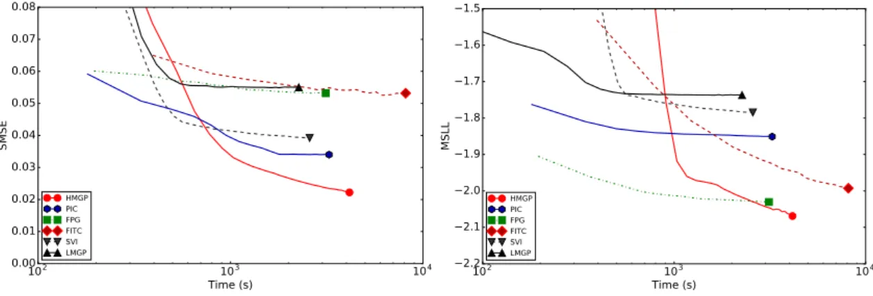
3.2 SMSE and MSLL as functions of training time for the apartment pricedataset for different GP approximation methods and different T values. Points on each line are annotated with the number of inducing points. Faster and more accurate approximation methods are located towards the bottom left corner of the plots. . . 47
3.3 Test results for motorcycle data using HMGP, FGP, FITC, PIC and full GP. Training data are marked with red crosses. Green dots are samples drawn from the predictive distribution evaluated at evenly spaced points (100 samples per point). Solid black line represents the predictive mean. In the top two figures, the predictive means by the two experts represented by red dashed and blue dotted lines are overlaid by the final combined predictive means (solid black line). See electronic color image. . . 48
3.4 Test results formotorcycle+sinedata using HMGP, FGP, FITC, PIC and full GP. Training data are marked with red crosses. Green dots are samples drawn from the predictive distribution evaluated at evenly spaced points (100 samples per point). Solid black line rep-resents the predictive mean. In the top two figures, the predictive means by the two experts represented by red dashed and blue dot-ted lines are overlaid by the final combined predictive means (solid black line). See electronic color image. . . 49
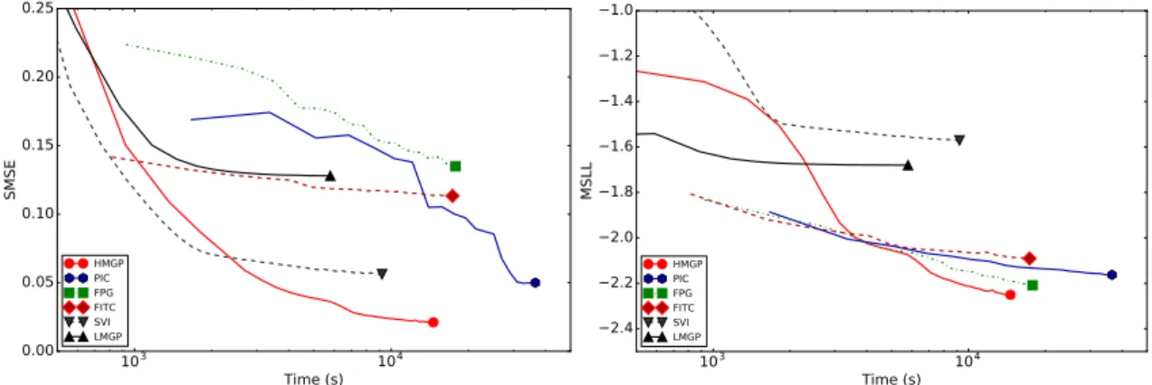
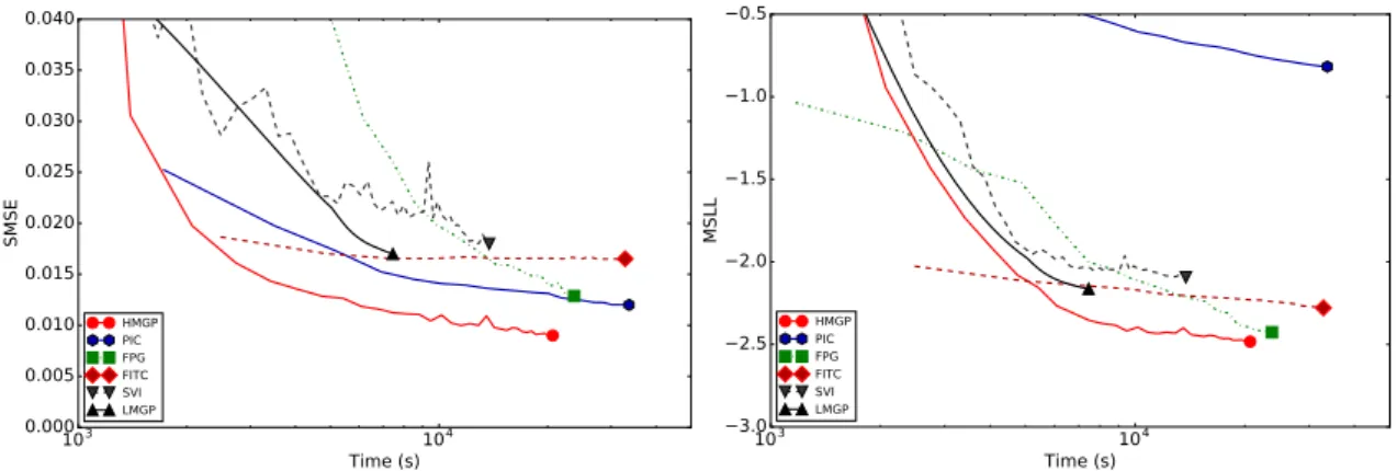
3.5 SMSE and MSLL as functions of training time for thekin40kdataset. 51
3.6 SMSE and MSLL as functions of training time for thepumadyn32nm dataset. Since the performance of PIC is very poor on this dataset, it has been removed from the plots to increase their resolutions. . . 52
List of Figures
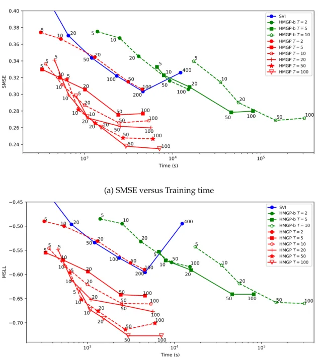
3.7 SMSE and MSLL as functions of training time for the pole-telecom dataset. . . 52
3.8 SMSE and MSLL as functions of training time for thechemdataset. 52
3.9 SMSE and MSLL as functions of training time for thesarcosdataset. 53
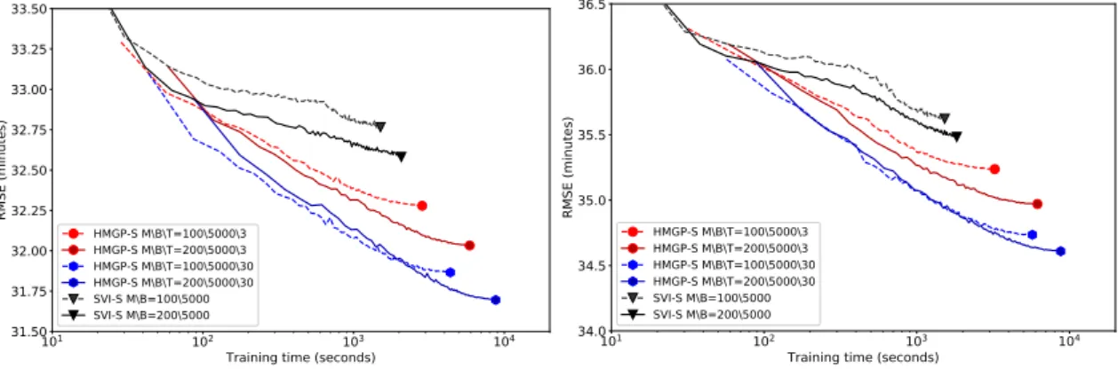
3.10 RMSE as a function of training time for the US flight dataset us-ing theFlight-700KandFlight-Allsplits for HMGP and SVI. Faster and more accurate approximation methods are located towards the bottom left corner of the plots. . . 58
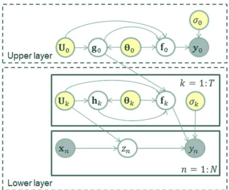
4.1 Schematic representation of the HGP model. Variable y0 denotes the vector of training outputs of the upper layer. zn is the expect indicator for the observation (xn,yn). Ul collectively denotes the inducing inputs of the l-th GP unit. For the c-th GP of the l-th GP unit, f(lc), gl(c), and θ(lc) denote the training latent variables, the inducing latent variables, and the hyper-parameters of covariance function, respectively. For thec-th GP of thek-th local GP unit,h(kc)
denotes the adjusted inducing latent variables. . . 68
4.2 Error rate and NLP as functions of training time on the WFRN dataset for SVGP and HGP with different initial number of experts T0. Faster and more accurate models are located towards the
bot-tom left corner of the plots. . . 84
4.3 Time-performance trade-offcurves of HGP, SVGP, VMGP and EP-FITC on theUSPS digitsdataset. . . 89
4.4 Time-performance trade-offcurves of HGP, SVGP and EP-FITC on the Spambase dataset. Performance of VMGP is too poor on this data, and hence, it is not included in the plots. . . 90
4.5 Error rates vs. training time on theUS flightdataset. . . 91
5.1 Structure of the hybrid deep learning-GP architecture for pedes-trian lane detection. . . 101
5.2 An encoder-decoder network with 3 encoder/decoder units. The
convolutional layers are denoted as “Convhkernel sizei-hnumber of channelsi”.
Max-pooling layers are denoted as “Pool hkernel sizei”.
Upsam-pling layers are denoted as “Up hkernel sizei”. Each Conv layer
has a stride of 1 pixel, and is immediately followed by a batch normalization layer and a ReLU layer. . . 102
5.3 Illustration of the operation of an upsampling layer. . . 105
5.4 The hierarchical GP classification model for pixel-wise lane seg-mentation. . . 106
List of Figures
5.5 Examples from the PLVP2 dataset. The first and third rows: Pedes-trian lane images. The second and forth rows: The ground-truth
masks for pedestrian lane segmentation. . . 110
5.6 Visual comparative results of different methods for pedestrian lane de-tection. Column 1: input images. Column 2: output of the Border-detection+segmentation method [1]. Column 3: output of SegNet [2]. Column 4: output of Bayesian SegNet [3]. Column 5: output of the pro-posed DL-HGP network. See the electronic color image. . . 117
5.7 Visual comparison of the pedestrian lane detection results (the detected lanes and the uncertainty maps) of Bayesian SegNet and the proposed DL-HGP network. Column 1: input images. Column 2 and 3: the detected lanes and the uncertainty maps by Bayesian SegNet.Column 4 and 5: the detected lanes and the uncertainty maps by the DL-HGP network. A brighter intensity in the uncertainty maps presents a higher uncertain levels. See the electronic color image.. . . 118
6.1 Examples of sonar snapshots in the three categories. . . 121
6.2 Structure of the proposed CNN-HGP architecture. . . 123
6.3 The proposed compact feature extractor. . . 124
6.4 Classification rates as a function of snapshot size (width). . . 126
6.5 The confusion matrices without and with normalization for the proposed hybrid model Hybrid 1B. . . 127
List of Tables
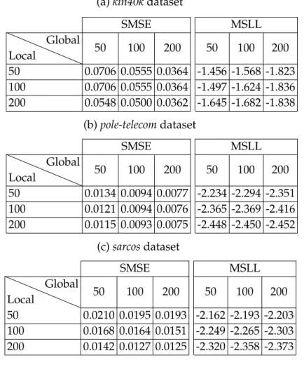
3.1 Performance of HMGP in terms of SMSE and MSLL using different numbers of global and local inducing points. . . 44
3.2 Test results, which include SMSE and MSLL, and training time (along with their respective standard deviations in brackets), for five different benchmark datasets:kin40k,pumadyn32nm,pole-telecom, chem andsarcos. Results are the averages over 5 trials, along with the standard deviation. The best performances are given in bold. . 53
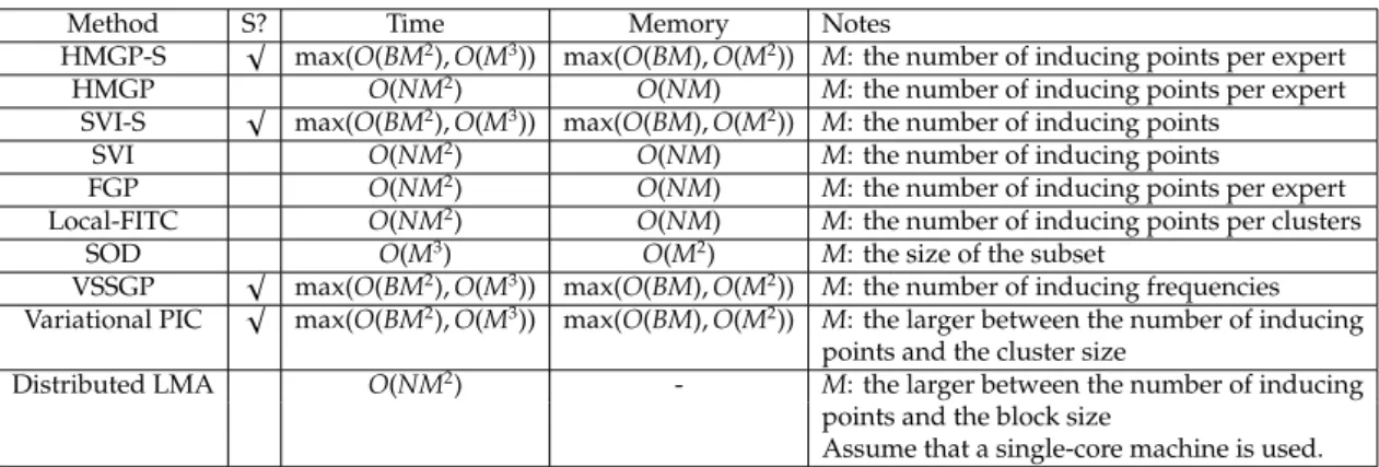
3.3 The time and memory complexity of several GP regression methods studied in Section 3.5.6. The second column indicates where the method is amendable to stochastic optimization. Nis the size of the training set. Bis the batch size when using stochastic optimization. 57
3.4 Performance (the average SMSE, MSLL and training time) of dif-ferent methods, on the Million Song dataset; the best performance is indicated in bold typeface. The numbers in brackets indicate the standard deviation over 5 runs. . . 57
3.5 Performances in terms of RMSE of different methods, on the US flightdataset; the best performances are indicated in bold typeface. The numbers in brackets indicate the standard deviation over 5 runs. Training time for each method includes time spent on clus-tering and model initialization. . . 59
4.1 Representative scalable approximation methods for GP classifica-tion. The mark ’-’ means that the non-conjugate approximation is combined with sparse approximation in a single variational infer-ence framework.. . . 65
List of Tables
4.2 Performance (error rate and NLP) of HGP using different numbers of global and local inducing points. MandPdenote the number of global and local inducing points in the percentages of the number of training samples, respectively. . . 83
4.3 Test results of HGP, SVGP, VMGP, EP-FITC, EP-GP, and SVM-RBF on nine different benchmark datasets. The best performances are shown in bold. The size and input dimension of each dataset are given under its name: (N\D). . . . . 87
4.4 Classification accuracy (in %) on ucf20 and ucf101 datasets, using Res3D and Res3D+iDT features. . . 92
4.5 Results (error rates) of different networks on theCIFAR-10dataset . 93
5.1 Statistics of the PLVP2 dataset. . . 109
5.2 Performance of different encoder-decoder network configurations for lane detection on the preliminary PLVP2 validation set. The listed number of parameters counts all the parameters of the encoder-decoder network and the GP classifier. . . 112
5.3 Performance of the DL-HGP network using different values for the initial number of GP expertsT0 on the preliminary PLVP2
valida-tion set. The configuravalida-tion C4K5 is used for the encoder-decoder network. . . 113
5.4 Performance of different lane detection methods on the PLVP2 dataset using 5-fold cross-validation. The deep learning based methods are placed into two different groups: those that use linear classifier, and those that use HGP classifier. . . 114
6.1 The number of sonar snapshots for experiments. . . 125
Acronyms
ARD Automatic relevance determination
CNN Convolutional neural network
EM Expectation maximization
EP Expectation propagation
FC Fully-connected
FGP Fast allocated mixture of GP experts
FITC Fully independent training conditional
GAN Generative adversarial network
GP Gaussian process
HGP Hierarchical Gaussian process classifier
HMGP Variational hierarchical mixture of GP experts
IVM Informative vector machine
KL Kullback-Leibler divergence
k-NN k-nearest neighbours
LMA Low-rank-cum-Markov approximation
MCMC Markov chain Monte Carlo
MoGPE Mixture of Gaussian process experts
MSLL Mean Standardized Log Loss
NLP Mean negative log predictive density
PIC Partially independent conditional
RMSE Root-Mean Square Error
RBF Radial basis function
SE Squared exponential
SMSE Standardized Mean Squared Error
SOD Subset of data points
SVGP Scalable variational sparse GP classifier
Acronyms
SVM Support vector machine
Abstract
Gaussian processes, which are distributions over functions, are powerful non-parametric tools for the two major machine learning tasks: regression and clas-sification. Both tasks are concerned with learning input-output mappings from example input-output pairs. In Gaussian process (GP) regression and classifica-tion, such mappings are modeled by Gaussian processes. In GP regression, the likelihood is Gaussian for continuous outputs, and hence closed-form solutions for prediction and model selection can be obtained. In GP classification, the like-lihood is non-Gaussian for discrete/categorical outputs, and hence closed-form solutions are not available, and approximate inference methods must be resorted. The main limitation of GP models is the high computational cost, which pre-vents their applications to large-scale datasets. Existing approximation methods to reduce the cost of GP models can be categorized into either global or local approaches; both approaches have their own shortcomings. Global approxima-tions, which summarize training data with inducing points, cannot account for non-stationarity and locality in complex datasets. Local approximations, which fit a GP for each sub-region of the input space, are prone to overfitting.
This thesis proposes scalable Gaussian process models for regression and clas-sification that effectively combine the advantages and overcome the shortcomings of both global and local GP approximations. The proposed models allow the uti-lization of both global and local information from the dataset through a two-layer hierarchical structure. The upper layer consists of a global sparse GP to coarsely model the entire dataset. The lower layer is composed of a mixture of GP experts which use local information to learn a fine-grained model. The key idea to avoid overfitting and to enforce correlation among the experts is to incorporate global information into their shared prior mean function. Model learning is performed through a variational inference algorithm which maximizes a lower bound of the log marginal likelihood. Our experiments on a wide range of benchmark datasets show that the proposed model for regression outperforms many state-of-the-art
Abstract
sparse GP regression methods, and that the model works well on large-scale problems using stochastic optimization.
For the proposed model for classification, we explicitly represent the varia-tional distributions of the inducing latent variables so that the model conditioned on these variables factorizes in the observations, and thus, the computation related to the log-likelihoods in the objective function involves only one-dimensional integrals. They can be computed efficiently without a separate non-conjugate approximation, which is often required for GP classification to deal with the non-Gaussian likelihood. Experimental results on a wide range of benchmark datasets demonstrate the advantages of the proposed model, as a stand-alone classifier or as the top layer of a deep neural network, in terms of scalability and predictive power.
The proposed GP classifier is applied to two practical machine learning prob-lems: pedestrian lane detectionandunderwater mine sensing in sonar imagery. For the pedestrian lane detection problem, the proposed GP binary classifier is combined with a compact convolutional encoder-decoder network to segment scene images into pedestrian lane and background regions. Evaluated on a pedestrian lane detection dataset of 5000 images, the proposed method gives more accurate lane detection compared to several existing methods. For the underwater mine sens-ing in sonar imagery, the proposed GP multi-class classifier is placed on top of a compact convolutional neural network to form a hybrid network, which can be trained end-to-end to classify rectangular regions of a sonar image into three cate-gories. Experimental results on real sonar images show that the proposed method achieves a significantly higher overall classification rate than other state-of-the-art techniques.
Acknowledgments
This thesis would not have been possible without the kind help, support, and guidance of many people who in one way or another inspired me and contributed their valuable assistance in the preparation and successful completion of this study.
First and foremost, I would like to gratefully acknowledge the enthusiastic supervision of my principal supervisor Prof. Abdesselam Bouzerdoum and my co-supervisor Dr. Son Lam Phung during this work. I would like to thank them for all their encouragement, support, invaluable guidance and valuable insights in the relevance of the study.
Secondly, I also thank the staffof School of Electrical, Computer, and Telecom-munications Engineering for giving me personal and professional support during my studies at University of Wollongong.
Thirdly, I would like to recognize that this research is supported in part by a grant from Australian Research Council.
Fourthly, I would like to thank to my fellow research students and friends, who have helped me during my studies at the university.
Last but not the least, I would like to express my gratitude to my beloved Parents, Husband, and Brother for their endless support and encouragement throughout my studies and research projects. I thank my daughter Nha Khanh for being my inspiration.
Chapter
1
Introduction
Chapter contents
1.1 Research objectives . . . . 1 1.2 Research contributions . . . . 2 1.3 Publications . . . . 3 1.4 Thesis structure . . . . 41.1
Research objectives
Gaussian process (GP) models are powerful non-parametric tools for Bayesian regression and pattern classification — the two tasks that are central to many machine learning problems. We can identify the two most desirable properties of GP models. First, due to its non-parametric nature, a GP has only a few hyper-parameters that need to be learned; thus, overfitting in model selection can be avoided. Second, GPs offer probabilistic prediction with well-calibrated uncertainty - a parameter that is negatively correlated to the confidence with which we can trust the predictive output.
In their standard form, GP models in general suffer from high computational complexity, which prevents their applications to large-scale datasets. Existing approximation methods to reduce the cost of GP models can be categorized into either global or local approaches. Global approximation methods summarize the entire dataset with a smaller set of inducing points [4,5,6,7,8,9,10,11,12]. These methods cannot account for non-stationarity and locality in complex datasets. Local approximation methods fit a GP model for each subset of data [13, 14, 15, 16, 17, 18, 19]. They overcome the above problem of global approximations, however, they are prone to overfitting.
1.2. Research contributions
The overall objective of this research is to develop scalable Gaussian process models for regression and classification that effectively combine the advantages of both global and local GP approximations. The proposed models allow the uti-lization of both global and local information from the dataset through hierarchical structures.
The specific aims of this research project are to:
• Provide a review of Gaussian process models and their applications for
regression and classification.
• Develop a scalable hierarchical Gaussian process model for regression.
• Develop a scalable hierarchical Gaussian process model for classification.
• Apply the proposed GP models into two practical machine learning
prob-lems, pedestrian lane detection and underwater mine sensing in sonar im-agery.
1.2
Research contributions
The principal contributions of this thesis are listed as follows:
• A literature review on GP regression and classification is presented with the
following key components: an overview of Gaussian processes and their theoretical background, the GP models for regression, and the GP models for classification together with the Gaussian approximation methods to deal with the non-conjugate likelihoods in GP classification.
• A novel scalable hierarchical Gaussian process model is proposed for
re-gression. The proposed method exploits both the global and local informa-tion from the training data through a hierarchical structure in a variainforma-tional framework. It can be trained with stochastic optimization for large-scale problems.
• A scalable hierarchical Gaussian process model is proposed for pattern
clas-sification. We first develop the model for multi-class classification, and subsequently present the model for binary classification as a special case of multi-class classification.
• The proposed GP model for binary classification is applied to the problem
of pedestrian lane detection. A hybrid deep learning-GP network, which combines a convolutional encoder-decoder network with the proposed GP
1.3. Publications
binary classifier, is developed to classify each pixel of a scene image into one of two classes: pedestrian lane or background. The network can be trained in an end-to-end manner.
• The proposed GP model for multi-class classification is applied to the
prob-lem of underwater mine sensing in sonar imagery. The GP classifier is paired with a compact convolutional neural network to form a hybrid net-work, which can be trained end-to-end to classify rectangular regions of a sonar image into three categories: mine-like object, other significant object, and background.
1.3
Publications
Following is the list of publications arising from this PhD research project:
• T. N. A. Nguyen, A. Bouzerdoum, and S. L. Phung, “Stochastic variational
hierarchical mixture of sparse Gaussian processes for regression,” Machine Learning, vol. 107, no. 12, pp. 1947–1986, 2018.
• T. N. A. Nguyen, A. Bouzerdoum, and S. L. Phung, “Scalable hierarchical
mixture of Gaussian processes for pattern classification,”IEEE International Conference on Acoustics, Speech and Signal Processing, pp. 2466–2470, 2018.
• T. N. A. Nguyen, A. Bouzerdoum, and S. L. Phung, “Variational inference
for infinite mixtures of sparse Gaussian processes through KL-correction,” IEEE International Conference on Acoustics, Speech and Signal Processing, pp. 2579–2583, 2016.
Following is the list of papers that arise from this research project and are under review:
• T. N. A. Nguyen, A. Bouzerdoum, and S. L. Phung, “A scalable hierarchical
Gaussian process classifier,” under review at IEEE Transactions on Signal Processing, 2019: minor revision required.
• T. N. A. Nguyen, A. Bouzerdoum, and S. L. Phung, “Hybrid Deep
Learning-Gaussian Process Architecture for Pedestrian Lane Detection in Unstruc-tured Scenes,” under review at IEEE Transactions on Neural Networks and Learning Systems, 2019.
• T. N. A. Nguyen, A. Bouzerdoum, and S. L. Phung, “Underwater mine
sens-ing in sonar imagery with a compact deep learnsens-ing architecture for scarce data,” under review atIEEE International Conference on Image Processing, 2019.
1.4. Thesis structure
1.4
Thesis structure
The thesis is structured as follows:
• Chapter1introduces the research project, its objectives, and a summary of
the related publications.
• Chapter2reviews the literature on Gaussian process models and their
ap-plications for regression and classification.
• Chapter 3 presents the proposed scalable hierarchical Gaussian process
models for regression.
• Chapter 4 describes the proposed scalable hierarchical Gaussian process
models for classification. It first presents the proposed model for multi-class multi-classification, and then discuss the model for binary multi-classification as a special case of multi-class classification.
• Chapter5discusses the application of the proposed GP binary classification
model to the problem of pedestrian lane detection. A hybrid deep learning-GP architecture, which combines a convolutional encoder-decoder network with the proposed GP binary classifier, is developed for this application.
• Chapter 6 proposes a hybrid architecture, which combines the proposed
GP multi-class classifier with a compact convolutional neural network, for underwater mine sensing in sonar imagery.
• Chapter 7 summarizes the research findings and provides concluding
Chapter
2
Reviews of Gaussian process
regression and classification
Chapter contents
2.1 Overview of Gaussian processes . . . . 6
2.2 Gaussian process regression . . . . 8
2.2.1 Probabilistic model for GP regression . . . 8
2.2.2 Model selection . . . 9
2.2.3 Inference . . . 9
2.3 Gaussian process classification . . . 11
2.3.1 GP binary classification . . . 11
2.3.2 Model selection and inference. . . 12
2.3.3 Gaussian approximations . . . 13
2.3.4 GP multi-class classification . . . 17
2.4 Chapter summary. . . 18 In this research, we are concerned with supervised learning, which is the machine learning task of learning output mappings from example input-output pairs (the training dataset). Depending on the characteristics of the input-output, supervised learning problems can be further grouped into either regression (for continuous outputs) orclassification(for discrete/categorical outputs).
Gaussian process models are powerful non-parametric tools with many de-sirable properties for supervised learning. First, a GP model is non-parametric, which means that the complexity of the model grows as more data samples are seen. Also due to its non-parametric nature, a GP has only a few hyper-parameters
2.1. Overview of Gaussian processes
that need to be learned; thus, overfitting in model selection can be avoided. Sec-ond, being Bayesian probabilistic models, GPs offer full probabilistic predictions, each of which is associated with an uncertainty - a parameter that is negatively correlated to the confidence with which we can trust the predictive output. A well-calibrated uncertainty is very useful in many areas such as Bayesian opti-mization [20], reinforcement learning [21], and active learning [22]; it is especially important if the prediction is used for making critical decisions. Despite many attractive features, the main limitation of GP models is their high computational complexity, which prevents their applications to large-scale datasets.
This chapter is structured as follows. Section2.1give an overview of Gaussian processes. Section 2.2 introduces the application of GP models for regression. Section2.3reviews the application of GP models for classification.
2.1
Overview of Gaussian processes
A GP is a stochastic process (an infinite collection of random variables indexed by time or space), such that any finite number of those random variables have consistent joint Gaussian distributions. A Gaussian process can be considered as a generalization of a Gaussian probability distribution. While a probability distribution is a distribution over finite-dimensional random variables which are scalars or vectors, a stochastic process is a distribution over functions. Like a Gaussian distribution which is fully specified by a mean and a covariancce, a Gaussian process is fully specified by a mean function and a covariance function. We can think of a Gaussian process as an infinite set of random variables f(x) of real values, indexed by a continuous variablexfrom the subspaceX ⊂RD. This
Gaus-sian process describes the distribution over functions of the form: f(x) : X 7−→R.
We can write the Gaussian process as
f(x)∼ GP(m(x), κ(x,x0)), (2.1)
wherem(x) andκ(x,x0) are the mean and covariance functions of the GP, respec-tively. These mean and covariance functions are defined as
m(x)=E[f(x)], (2.2)
2.1. Overview of Gaussian processes
The covariance functionk(x,x’) is typically represented by a squared exponential (SE) kernel: κ(x,x0)=βexp −1 2(x−x 0 )TM(x−x0) , (2.4)
where β is the signal variance, and M = diag([φ1, ..., φD]) with φd = [`d]−2 and
`d being the variation length-scale for input dimension d, for d = 1, ...,D. The
hyperparameters β and M govern properties of sample functions. All the hy-perparameters of a covariance function are collectively represented by the vector θ. The covariance function given by Eq. (2.4) is also known as the squared exponential kernel with automatic relevance determination (SE-ARD) since the length-scales of different input dimensions are allowed to take different values, which determine the relevance of the input dimensions to the variation of func-tion variables. The SE covariance is a stafunc-tionary funcfunc-tion — a funcfunc-tion of (x−x’),
which is invariant to translations.
Suppose that we choose a finite subset of those function variables (random variables) f =
f1, f2, ..., fN , indexed by the corresponding subset of inputs
X={x1,x2, ...,xN}, where fi ≡ f(xi). According to the definition of GPs, any of
such subset of random function variables has a joint multivariate Gaussian distri-bution:
p(f|X)=N(mX,KXX), (2.5)
where mX denotes the vector formed by evaluating the function m(x) at all the input pointsxinX, andKXXdenotes the covariance matrix formed by evaluating κ(x,x0) at all pairs of input points inX. The entry of the covariance matrix at the (i, j) position —Ki jis the covariance of the two random function variables fi and
fj, and it is calculated as
Ki j =κ(xi,xj). (2.6)
Gaussian processes are conditional probabilistic models; it only models the conditional of the outputs given the inputsp(f|X), the distribution of the inputs
themselves p(x) is not specific. Throughout the thesis, for simplicity, we will neglect the explicit notational conditioning on the inputs, while understanding that the appropriate inputs are always conditioned on: p(f)≡p(f|X).
A requirement in the definition of Gaussian process is that these Gaussian distributions expressed in Eq. (2.5) are consistent, i.e., the usual rules of probability apply to the collection of random function variables. For example, the following
2.2. Gaussian process regression
marginalization rule applies:
p fi=
Z
pfi, fj
d fj. (2.7)
This means that if the GP specifiesp(fi, fj) =N(m,K), then it also impliesp(fi) =
N(mi,Kii), whereKiiis the relevant submatrix ofK. Notice that since the entries
of the covariance matrix are specified by the covariance function as in Eq. (2.6), the above consistency requirement is automatically fulfilled.
2.2
Gaussian process regression
In this section, we discuss the application of GP models for regression; this is the simplest form of Gaussian process models for supervised learning.
Consider a typical regression problem where a training set D hasN pairs of
D-dimensional inputs xn and one-dimensional outputs yn, i.e.,D = (xn,yn) Nn=1
with xn ∈ X ⊂ RD and yn ∈ R. Let X and y collectively represent the training
inputs and outputs, respectively: X={x1, ...,xN}andy=(y1, ...,yN)T. Our task is to
compute the outputsy∗
at new test locationsX∗, given the training dataXandy.
2.2.1
Probabilistic model for GP regression
In GP regression, we assume that there is an underlying latent function f(x) :
X 7−→Rwhich is priorly distributed according to a GP with mean and covariance
functions m(x) and κ(x,x0
): f(x) ∼ GP(m(x), κ(x,x0
)). Let fn denote f(xn), and f
denote the vector of latent function variables at the training inputs: f=[f1, ..., fN]T.
The GP places a Gaussian prior onf:
p(f)=N(f|mX,KXX). (2.8)
The observed outputynis then related to the latent variables fnby
yn= f(xn)+n, (2.9)
wherenis a zero-mean independent and identically distributed Gaussian noise
with varianceσ2, i.e.
n∼ N(0, σ2). The above relationship between ynand fncan
also be expressed in the form of a normal distribution as
2.2. Gaussian process regression
The likelihoodp(y|f) is then a factorized Gaussian:
p(y|f)=
N
Y
n=1
p(yn|fn)=N(f, σ2I). (2.11)
The two important aspects of GP regression are model selection, which is concerned with the selection of the model hyperparameters such as the hyperpa-rameters of the mean and covariance functions, and inference, which deals with making prediction. These two aspects are discussed in Sections2.2.2and2.2.3.
2.2.2
Model selection
Before the GP regression model can be used for prediction, the model hyper-parameters must be learned from the data. These hyperhyper-parameters include the hyperparameters of the mean function m(x) and covariance function κ(x,x0) as well as the noise varianceσ2. For that, the marginal likelihood (or the evidence)
p(y)=
Z
p(y|f)p(f)df. (2.12)
is maximized with respect to (w.r.t.) these hyperparameters. Since both the prior distributionp(f) (given in Eq. (2.8)) and the likelihoodp(y|f) (given in Eq. (2.11))
are Gaussian distributions, the marginal likelihood p(y) is also Gaussian. Using the general properties of Gaussian distributions given in Eq. (8.5), p(y) can be calculated in closed-form as:
p(y)=N(mX,K
XX+σ2I). (2.13)
2.2.3
Inference
Inference deals with making predictions at new test points. Let look at a set of test pointsX∗, and their corresponding latent function variablesf∗and outputsy∗
. LetKAB denote a covariance matrix formed by evaluating the functionκ(x,x
0 ) at all pairs of points (x,x0) with x inA and x0 inB. The property of GP gives the following joint prior distribution forfandf∗:
f f∗ ∼ N mX mX∗ , KXX KXX∗ KX∗X KX∗X∗ (2.14)
2.2. Gaussian process regression
Using the Gaussian identities presented in Appendix8.1.1, the predictive distri-bution forf∗given the noise-free observationsfcan be computed as:
p(f∗|f)=NKX∗ XK −1 XX(f−mX)+mX∗, KX∗X∗ −KX∗XK −1 XXKXX∗ (2.15)
In realistic situations, we do not have access to the function valuesfbut the noisy observation y. To make prediction for f∗ using y, we first derive the joint prior distribution fory andf∗. This can be done by replacing the term corresponding top(f) in Eq. (2.14) with that ofp(y):
y f∗ ∼ N mX mX∗ , KXX+σ2I KXX∗ KX∗X KX∗X∗ (2.16)
Finally, the predictive distribution for the test latent variables (noise-free outputs)
f∗givenycan be computed as:
p(f∗|y)=NKX∗X[K XX+σ2I] −1 (y−mX)+mX∗, KX∗X∗ −KX∗X[KXX+σ2I] −1 KXX∗ (2.17)
The predictive distribution for noisy test datay∗is calculated by marginalizing out the test latent variablesf∗:
p(y∗|y)=
Z
p(y∗|f∗)p(f∗|y)df∗. (2.18)
This is equivalent to simply adding the noise varianceσ2to the predictive variance
off∗as follows: p(y∗|y)=NKX∗X[K XX+σ2I] −1 (y−mX)+mX∗, KX∗X∗ −KX∗X[KXX+σ2I] −1 KXX∗ +σ2I (2.19)
Note that by subtracting offset and simple trends from the data before model-ing, we can assume, without loss of generality, that the prior mean functionm(x) is equal to0. For notational simplicity, we will take the mean function to be zero hereinafter, unless otherwise stated.
The dominant cost in GP inference is the inversion of the covariance matrix [KXX+σ2I] in Eqs. (2.13) and (2.17), which requires a computational time ofO(N3). In addition, the storage of the covariance matrix requires a memory complexity ofO(N2). These computational costs are prohibitive for large datasets. We will
2.3. Gaussian process classification
discuss the approximation methods to reduce the computational cost for GP regression in Chapter3.
2.3
Gaussian process classification
In this section, we review the application of Gaussian process models for classifi-cation problems, in which we wish to assign an input pattern to one ofCclasses. Even though, we can view both classification and regression as function approx-imation problems, the solution for the GP classification is more demanding than that for the GP regression considered in Section2.2. This is because for regression, a Gaussian likelihood function is assumed; it is combined with a Gaussian process prior to give rise to a Gaussian posterior distribution over function variables, and everything remains analytically tractable. For classification, where the outputs are discrete class labels, the Gaussian likelihood is inappropriate. Therefore, exact inference is not feasible, and approximate inference must be resorted.
We first focus our discussion on Gaussian process models for binary classifi-cation, in which samples are classified into one of the two classes. We then extend the discussion to Gaussian process models for multi-class classification, in which there are more than two classes.
2.3.1
GP binary classification
Consider a typicalbinaryclassification problem, and letD=
(xn,yn) Nn=1denote a
training set ofN pairs of input pointsxn ∈ X ⊂ RD and class labels yn ∈ {−1,1}.
Let X and ycollectively represent the training inputs and outputs, respectively:
X = [x1, ...,xN]T and y =[y1, ...,yN]T. The classification task is to compute the
outputy∗
at new test locationsx∗
, givenXandy.
Similar to the case of GP regression, in GP classification, we also assume that there is an underlying latent function f(x) : X 7−→ R, which follows a GP prior,
i.e., f(x) ∼ GP(0, κ(x,x0
)). Let fn denote f(xn), and f denote the vector of latent
function variables at the training inputs: f=[f1, ..., fN]T. The GP places a Gaussian
prior onfas follows:
p(f)=N(f|0,KXX). (2.20)
The latent function variablefis then related to the observed outputs according to a predefined likelihood distributionp(yn|fn). In particular, the latent function is first
mapped into the unit interval through a sigmoidal inverse-link function sig(f) :
R7−→[0,1], such that the class probabilityp(yn = +1|fn) can be written as sig(fn).
2.3. Gaussian process classification
then the likelihood that relates the observed outputs and the transformed latent function values can be compactly written as
p(yn|fn)=sig(ynfn). (2.21)
Equation (2.21) implies that the class membership probability can be calculated as p(yn = 1|fn) = sig(fn) and p(yn = −1|fn) = sig(−fn) = 1− sig(fn). The two
most commonly used sigmoidal inverse-link functions are the logistic function sig(z)=λ(z)=1/(1+exp(−z)), and theprobitfunction sig(z)=φ(z)=Rz
−∞N(x|0,1)dx. The class labels are independently distributed given the latent function f, and hence, the likelihoodp(y|f) is factorized as
p(y|f)= N Y n=1 p(yn|fn)= N Y n=1 sig(ynfn). (2.22)
2.3.2
Model selection and inference
Like in the case of GP regression, the two most important aspects for GP classi-fication are inference and model selection, which require the computation of the posterior distribution of the latent function variables and the marginal likelihood, respectively. However, due to the non-Gaussian likelihood, these calculations are not analytically tractable, and approximations are often resorted. In this sub-section, we first introduce the formulation of the exact terms required for model selection and inference, before discussing the different methods for their approx-imations in Subsection2.3.3.
Model selection: Model selection in GP classification involves finding the model hyperparameters such as the parameters of mean and covariance functions. For that, the marginal likelihood (or evidence)
p(y)=
Z
p(y|f)p(f)df (2.23)
is maximized with respect to (w.r.t.) the model hyperparameters.
Inference: Inference deals with making prediction given the training data. Prediction at test inputx∗
can be calculated as p(y∗|y)= Z p(y∗|f∗)p(f∗|y)d f∗= Z p(y∗|f∗) "Z p(f∗|f)p(f|y)df # d f∗. (2.24) The termp(f∗|
f) for GP classication can be derived in the similar way as that for GP regression, which are previously given in Eq. (2.15):
2.3. Gaussian process classification p(f∗|f)=N(Kx∗ XK −1 XXf, Kx∗x∗ −Kx∗XK −1 XXKXx∗). (2.25)
The main object of interest for the inference in (2.24) is the posterior over latent function valuesp(f|y), which is given by
p(f|y)=p(y|f)p(f)/p(y). (2.26)
2.3.3
Gaussian approximations
Since the likelihoodp(y|f) is non-Gaussian, the Gaussian process priorp(f) is
non-conjugate to the likelihood. Therefore, the marginal likelihood given in (2.23) and the posterior given in (2.26) are not analytically tractable. To obtain exact answers, we can use Markov chain Monte Carlo (MCMC) sampling algorithms, which are very costly. However, if the sigmoid function sig is concave in the log-arithmic domain, the posterior can be shown to be unimodal, and thus Gaussian approximations to the posterior can be employed as alternatives to MCMC.
Let’s assume that such a Gaussian approximation to the posterior has been found with mean m and covariance V, i.e. p(f|y) ≈ q(f) = N(f|m,V). As
a result, the latent distribution at the test point x∗ becomes tractable p(f∗| y) = R p(f∗| f)p(f|y)df=N(f∗| m∗, v∗ ) with m∗=Kx∗ XK −1 XXm, (2.27) v∗=Kx∗ x∗ −K x∗X(K−1 XX−K −1 XXVK −1 XX)KXx∗. (2.28)
Note that the general properties of the Gaussian distributions presented in Appendix 8.1.2 is used to derive the above formulation of p(f∗|
y). The last step for making prediction is to calculate the one dimensional integral p(y∗|y) =
R
p(y∗|f∗)p(f∗|y)d f∗. For the probit likelihood, this integral can be computed
analyt-ically. For the logistic likelihood, sampling methods or analytical approximations are required to compute this one-dimensional integral.
Next, we discuss three most popular methods to approximate the posterior p(f|y): Laplace approximation, expectation propagation, and KL-divergence
mini-mization (also known as variational inference). These methods can also be referred to as non-conjugate approximations.
2.3.3.1 Laplace approximation (LA)
Posterior: In Laplace approximation method, a second order Taylor expansion of the log posterior lnp(f|y) around the maximum of the posterior (the posterior
2.3. Gaussian process classification
mode) is used to construct the following Gaussian approximation:
p(f|y)≈q(f)=N(f|m,A−1)∝exp
−1
2(f−m)
TA(f−m), (2.29)
wherem = argmaxfp(f|y) is the posterior mode, andA = −∇∇lnp(f|y)|f=mis the
Hessian of the negative log posterior at that point.
Since the termp(y) in the posteriorp(f|y) =p(y|f)p(f)/p(y) is independent off,
we only need to maximize the unnormalized posteriorp(y|f)p(f) or its logarithm Ψ(f)=lnp(y|f)p(f) with respect tof. As shown in Chapter 3 of [23]
Ψ(f)=lnp(y|f)− 1 2f TK−1 XXf− 1 2|KXX| − N 2 ln(2π), (2.30)
the modemcan be found using Newton’s method, and Hessian matrixAis
A=K−XX1 +W, (2.31) where W=− ∂ 2lnp(y|f) ∂f∂fT f=m . (2.32)
Due to the factorial structure of the likelihood, matrixWturns out to be diagonal with itsi-th diagonal element given by
Wii=− ∂2lnp(y i|fi) ∂f2 i fi=m i . (2.33)
Log marginal likelihood: Lethdenote the log value of the unnormalized posterior p(y|f)p(f) at its modem: h = Ψ(m). A Taylor expansion of Ψ(f) is then given by Ψ(f)≈h−1
2(f−m)T(K
−1
XX+W)(f−m). Consequently, substituting this approximation ofΨ(f) into Eq. (2.23) gives an approximation of the log marginal likelihood
lnp(y)=ln Z exp(Ψ(f))df (2.34) ≈lnp(y|f)| f=m− 1 2m TK−1 XXm+ 1 2ln|I+KXXW| (2.35) The problem with LA is that the Hessian (evaluated at the mode) may give very poor approximation to the true shape of the posterior. The peak of the posterior could be much broader or narrower than the Hessian indicates. In addition, it could be a skew peak, while LA assumes that the posterior has elliptical contours
2.3. Gaussian process classification
around the peak.
2.3.3.2 Expectation propagation (EP)
Expectation propagation [24] is an iterative method to find approximation based on approximate marginal moments. To apply EP to GP classification, each indi-vidual likelihood term is replaced by a site functionti(fi), which is a unnormalized
Gaussian
p(yi|fi)≈ti(fi, µi, σ2i,Zi),ZiN(fi|µi, σ2i) (2.36)
such that the moments of the approximate marginalq(fi),
R
p(f)QN
j=1ZjN(fj|µj, σ2j)d j
agree with those of the approximate marginal ˆq(fi),
R
p(f)p(yi|fi)Qj,iZjN(fj|µj, σ 2
j)d j,
in which the exact likelihood termp(yi|fi) is used. The details on EP approximation
for GP classification can be found in Chapter 3 of [23].
Posterior: Based on the local approximations, the approximate posterior can be given by p(f|y)≈ N(f|m,V)=Nf|m,(K−1 XX+W) −1 , (2.37) where W=[σ−i2]ii, (2.38) m=VWµ, (2.39) µ=(µ1, ..., µN)T. (2.40)
Log marginal likelihood: The approximate log marginal likelihood is given by
lnp(y)=ln Z p(y|f)p(f)df ≈ln Z N Y i=1 ti(fi, µi, σ2i,Zi)p(f)df = N X i=1 lnZi− 1 2µ T (KXX+W −1 )−1µ− 1 2ln|KXX+W −1| − N 2 ln(2π). (2.41) The convergence of EP is not generally guaranteed, but for the case of log-concave likelihood functions in GP classification, Nickisch and Rasmussen always observe its convergence through their experiments in [25]. The experimental findings in [25] also suggest that the approximate log marginal likelihood given by EP is in general close to the true log marginal likelihood.
2.3. Gaussian process classification
2.3.3.3 KL-divergence minimization (KL)
This KL-divergence minimization method is also known as variational inference (VI). This method aims to minimize the following reverse KL-divergence between the approximate posteriorq(f)= N(f|m,V) and the exact posteriorp(f|y) w.r.t. m
andV:
K L(q(f)||p(f|y))=
Z
N(f|m,V) lnN(f|m,V)
p(f|y) =:K L(m,V). (2.42)
It has been shown in [25] that
K L(m,V)=− N X i=1 Z N(fi|mi,vii) ln sig(yifi)d fi −1 2ln|V|+ 1 2m TK−1 XXm+ 1 2Tr(K −1 XXV), (2.43)
after dropping the constant terms w.r.t. mandV. Leta(m,V) denote the first term ofK L(m,V). At the optimum, the derivatives ofK L(m,V) w.r.t. m and V are
equal to zero: ∂K L ∂m =− ∂a ∂m +K −1 XXm=0 =>m=KXX ∂a ∂m =KXXα, (2.44) ∂K L ∂V =− ∂a ∂V − 1 2V −1 + 1 2K −1 XX =0=>V= K −1 XX−2 " ∂a ∂vii # ii !−1 = K−XX1 −2Λ −1 . (2.45) Two new parametersα andΛ are defined in the above equations. Plugging the expressions (2.44) and (2.45) into Eq. (2.43) gives the expression for KL-divergence in terms of α and Λ: K L(α,Λ). From there, α and Λ can be estimated using
Newton’s method.
Note that if we directly mimimize K L(m,V) w.r.t. m and V, then there
are in principle O(N2) parameters to be optimized. Re-parameterizing the
KL-divergence in terms ofαandΛ, we are optimizing only 2Nfree parameters since Λis a diagonal matrix.
Posterior: The posterior p(f|y) is approximated by q(f) = N(f|m,V), wherem
andVare given in Eqs. (2.44) and (2.45) based on the estimation ofαandΛ. Log marginal likelihood: The log marginal likelihood can be written as
lnp(y)= Z q(f) ln ( p(y|f)p(f) q(f) ) df+K L(q(f)||p(f|y))=L+K L(q(f)||p(f|y)), (2.46)
which definesL. Since the KL-divergence is non-negative,Lis a lower-bound of
2.3. Gaussian process classification
to maximizing the boundL, resulting in a tight lower-bound for the log marginal
likelihood. It is used as the approximation to the log marginal likelihood for model selection. However, this lower boundLis known to be below the approximation
for the log marginal likelihood obtained by EP ([26], page 2183).
2.3.4
GP multi-class classification
Consider a multi-class classification problem, where an input pattern are clas-sified into one of C classes, i.e., the outputs receive integer values from 1 to C. To apply GP to that classification problem, we use C latent functions (one for each class). The latent function associated with class c is denoted as f(c)(x);
it is priorly distributed according to a GP with covariance function κ(c)(x,x0 ): f(x)∼ GP(0, κ(c)(x,x0
)). In the following, we use the superscript (c) to denote class c.
Each class observation is now dependent on the latent variables from all the C latent functions. Let fn denote the vector of the latent variables at input xn,
i.e., fn = (fn(c))Cc=1 where f (c)
n ≡ f(c)(xn). The observed output yn is then related to
the corresponding latent function variables fn through the following likelihood
function:
p(yn|fn)=Cat(S(fn)).
Here, Cat is a categorical distribution, andSis a mapping fromRCto the relevant
probability simplex. For each input vectorfn, the mapping Sgenerates a vector
ofCelements (π(nc))Cc=1 such that
PC c=1π (c) n =1, and 0 ≤π (c) n ≤ 1 forc =1, ...,C. The
resultingπ(nc)is the class membership probability for classc.
The most popular mapping S for GP multi-class classification is the softmax
function, which is defined as
π(c) n =S(fn)c= exp (fn(c)) PC c0= 1exp (f (c0 ) n ) . (2.47)
The class labels conditioned on the latent function variables are independently distributed, i.e., the overall likelihoodp(y|f) is factorized as
p(y|f)=
N
Y
n=1
p(yn|fn). (2.48)
Like in GP binary classification, since the likelihood in GP multi-class classification is non-Gaussian, the posterior of latent variables and the marginal likelihood are
2.4. Chapter summary
not analytically tractable. Therefore, Gaussian approximation methods such as Laplace approximation, expectation propagation, and KL-divergence minimiza-tion can be resorted to approximate the posterior and marginal likelihood in GP multi-class classification, in the similar ways to those used in GP binary classifi-cation. The interested reader is referred to [23] for more details on GP multi-class classification.
2.4
Chapter summary
This chapter presented a literature review on Gaussian process models and their applications for regression and classification. After giving an overview of Gaus-sian processes, we described the GP models for regression, and the GP models for classification together with the Gaussian approximation methods to deal with the non-conjugate likelihoods in GP classification.
Chapter
3
Stochastic Variational Hierarchical
Mixture of Sparse Gaussian Processes
for Regression
Chapter contents
3.1 Introduction . . . 20
3.2 Related work on approximation for Gaussian process regression 23
3.2.1 Overview of sparse GP approximation . . . 23
3.2.2 Sparse GP approximation based on variational inference . 25 3.2.3 Local approximations . . . 26
3.2.4 Combine local and global GP approximations . . . 27
3.3 Variational hierarchical mixture of Gaussian process experts . . 28
3.4 Inference . . . 31
3.4.1 The evidence lower bound . . . 31
3.4.2 The variational inference algorithm . . . 35 3.4.3 Computational complexity and cost reduction
approxi-mation . . . 37
3.4.4 Stochastic optimization . . . 39 3.4.5 Prediction . . . 40
3.5 Experiments . . . 41
3.5.1 Experimental methods . . . 42
3.5.2 Experiments with varying number of inducing points . . . 43 3.5.3 Experiments with varying number of experts . . . 45
3.1. Introduction
3.5.4 Experiments on small-sized datasets . . . 46
3.5.5 Experiments on medium-sized datasets . . . 50 3.5.6 Experiments on large datasets . . . 54
3.6 Chapter summary. . . 60
Chapter3has been published in our paper
T. N. A. Nguyen, A. Bouserdoum, and S. L. Phung, “Stochastic variational hierarchical mixture of sparse Gaussian processes for regression,” Machine Learning, vol. 107, no. 12, pp. 1947–1986, 2018.
Gaussian process models have become the dominant approach to nonparamet-ric Bayesian regression, but their limitation is the high computational cost. Exist-ing approximation methods to reduce the cost of GP regression can be categorized into either global or local approaches. Global approximations, which summarize training data with inducing points, cannot account for non-stationarity and local-ity in complex datasets. Local approximations, which fit a GP for each sub-region of the input space, are prone to overfitting. In this chapter, we propose a scalable Gaussian process regression method that combines the advantages of both global and local GP approximations through a two-layer hierarchical model using a vari-ational inference framework. The upper layer consists of a global sparse GP to coarsely model the entire dataset, whereas the lower layer comprises a mixture of sparse GP experts which exploit local information to learn a fine-grained model. A two-step variational inference algorithm is developed to learn the global GP, the GP experts and the gating network simultaneously. Stochastic optimization can be employed to allow the application of the model to large-scale problems. Experiments on a wide range of benchmark datasets demonstrate the flexibility, scalability and predictive power of the proposed method.
3.1
Introduction
Gaussian process models have become the dominant approach to nonparametric Bayesian regression [27,28,29,30,31,32]. However, GP models in general suffer from high computational complexity, which is O(N3) in training time and and O(N2) in memory for N training data points. These computation costs arise
mainly from the inversion and storage of the covariance matrix. The unfavorable complexity prevents the application of GP regression to large-scale datasets.
There has been much interest in sparse approximation methods for GPs to overcome the limitation of high computational cost [4, 5, 6, 7, 8, 9, 10]. A com-prehensive review of many popular sparse approximation methods can be found
3.1. Introduction
in [33]. In these methods, the entire training set is approximated using a small set of inducing points. The covariance matrix among all data points is thereby approximated by a low-rank one. In this way, a lower complexity of O(NM2)
in training time and O(NM) in memory is achieved, whereM is the number of inducing points. However, even these reduced storage methods are prohibitive for big data that contain millions or billions of samples.
There are generally two approaches to scale up sparse GP models to be able to handle big data. One approach is to spread computation across many nodes in a distributed system [34, 35]. This approach often requires abundant com-putational resources (processors and memory) though. Another approach is to learn sparse GP models in stochastic fashion, where a mini-batch of data is used at each optimization iteration. Examples for this approach are [36] and [37], in which stochastic variational inference [38] is employed for model learning. This approach allows the application of sparse GP regression to large-scale problems even with limited available resources.
The sparse GPs normally work well for simple datasets. However, in complex datasets, the dependencies among the observations cannot be well-captured by a small number of inducing points. In addition, a single GP accompanied by a small set of global inducing points cannot account for the non-stationarity and locality in such datasets, as argued in [13]. Mixture of Gaussian processes is another approach to reduce the computational complexity of GPs as presented in [13,14,15,16,17,18,19]. In the mixture of GPs approach, a gating network divides the input space into regions within which a specific GP expert is responsible for making predictions. In this way, the computational complexity is reduced since the storage and inversion of a large covariance matrix are replaced by those of multiple smaller matrices. The non-stationarity and locality in the data can also be naturally addressed.
Mixtures of GPs have two main limitations. The first limitation is the com-plexity of the inference problem, which usually involves simultaneous learning of both the experts and the gating network. Therefore, approximation techniques are often required for the inference. Many existing mixtures of GPs, such as those in [13, 15, 16, 17], resort to the intensive Markov chain Monte Carlo (MCMC) sampling methods, which can be very slow, especially for large-scale datasets. As a result, the limited scalability prohibits their application to even moderate-sized problems. Recently, several variational mixtures of GP experts have been pro-posed for GP regression using variational inference, which is a more flexible and faster alternative to MCMC sampling [18, 19,39]. However, there is still no clear way to apply stochastic optimization to variational mixtures of GPs to enable their
3.1. Introduction
application to big data. To the best of our knowledge, the largest experiments using the existing variational GP mixtures have been performed in [19] and [40] with 100,000 data points. The second limitation of mixtures of GPs is that each expert is independently trained using only the local data assigned to it, without taking into account the global information, i.e. the correlations between clusters. The trained experts are therefore likely to overfit to the local training data.
In this chapter, we propose a GP approximation method for regression that combines the advantages of sparse approximation and mixture of GPs in a varia-tional inference framework to exploit both the global and local information from the training data. Our model has a two-layer hierarchical structure. The upper layer uses a sparse GP accompanied by a set of global inducing points to coarsely model the entire dataset. The lower layer comprises a mixture of GP experts, each of which is also a sparse GP. These experts make use of the local information from the corresponding data points assigned to them for fine-grained modeling. The experts share a common prior mean function which is the latent function modeled by the upper layer in order to enforce correlation among themselves. This way, overfitting is avoided. For inference, we develop a two-step variational inference algorithm for simultaneous learning of the global sparse GP, the experts and the gating network. We also derive an objective function that appears in a factorized form necessary for stochastic optimization, thereby enabling the application of the model to large-scale datasets.
For the experiments and validation, we consider three sets of experiments with datasets of varying size to investigate different aspects of the proposed model. In the first set of experiments, we visually investigate the model on two small-size datasets with input-dependent noise. The result shows that the proposed method is able to both detect the common trend and handle the non-stationarity in the datasets at the same time. In the second set of experiments, we evaluate the predictive performance of the proposed model and compare it with those of four other baseline models, using five medium-sized benchmark datasets. These baselines include [10], [36], [19] and [41]. The proposed model outperforms with statistical significance all the other baselines in 4 out of 5 datasets. Finally, we compare the proposed method to the GP with stochastic variational inference (SVI) [36] on large-scale datasets with up to 2 million samples when stochastic optimization is enabled. The proposed method is shown to outperform SVI in terms of the accuracy-time trade-off.
The rest of the chapter is organized as follows. Section 3.2 gives a review of the related work on sparse approximation for Gaussian process regression. Section3.3presents our proposed model: a variational hierarchical mixture of GP
3.2. Related work