Lifting from the Deep: Convolutional 3D Pose Estimation from a Single Image
Denis Tome
University College London
[email protected]
Chris Russell
The Turing Institute and
The University of Edinburgh
[email protected]
Lourdes Agapito
University College London
[email protected]
http://visual.cs.ucl.ac.uk/pubs/liftingFromTheDeep
Abstract
We propose a unified formulation for the problem of 3D human pose estimation from a single raw RGB image that reasons jointly about 2D joint estimation and 3D pose reconstruction to improve both tasks. We take an inte-grated approach that fuses probabilistic knowledge of 3D human pose with a multi-stage CNN architecture and uses the knowledge of plausible 3D landmark locations to refine the search for better 2D locations. The entire process is trained end-to-end, is extremely efficient and obtains state-of-the-art results on Human3.6M outperforming previous approaches both on 2D and 3D errors.
1. Introduction
Estimating the full 3D pose of a human from a single RGB image is one of the most challenging problems in computer vision. It involves tackling two inherently am-biguous tasks. First, the 2D location of the human joints, or landmarks, must be found in the image, a problem plagued with ambiguities due to the large variations in visual ap-pearance caused by different camera viewpoints, external and self occlusions or changes in clothing, body shape or illumination. Next, lifting the coordinates of the 2D land-marks into 3D from a single image is still an ill-posed prob-lem – the space of possible 3D poses consistent with the 2D landmark locations of a human, is infinite. Finding the correct 3D pose that matches the image requires injecting additional information usually in the form of 3D geometric pose priors and temporal or structural constraints.
We propose a new joint approach to 2D landmark de-tection and full 3D pose estimation from a single RGB im-age that takes advantim-age of reasoning jointly about the es-timation of 2D and 3D landmark locations to improve both tasks. We propose a novel CNN architecture that learns to combine the image appearance based predictions provided
by convolutional-pose-machine style 2D landmark
detec-tors [44], with the geometric 3D skeletal information
en-coded in a novel pretrained model of 3D human pose. Information captured by the 3D human pose model is embedded in the CNN architecture as an additional layer that lifts 2D landmark coordinates into 3D while impos-ing that they lie on the space of physically plausible poses. The advantage of integrating the output proposed by the 2D landmark location predictors – based purely on image ap-pearance – with the 3D pose predicted by a probabilistic model, is that the 2D landmark location estimates are im-proved by guaranteeing that they satisfy the anatomical 3D constraints encapsulated in the human 3D pose model. In this way, both tasks clearly benefit from each other.
A further advantage of our approach is that the 2D and 3D training data sources may be completely independent. The deep architecture only needs that images are annotated with 2D poses, not 3D poses. The human pose model is trained independently and exclusively from 3D mocap data. This decoupling between 2D and 3D training data presents a huge advantage since we can augment the training sets completely independently. For instance we can take advan-tage of extra 2D pose annotations without the need for 3D ground truth or extend the 3D training data to further mocap datasets without the need for synchronized 2D images.
Our contribution:In this work, we show how to integrate a prelearned 3D human pose model directly within a novel
CNN architecture (illustrated in figure1) for joint 2D
land-mark and 3D human pose estimation. In contrast to pre-existing methods, we do not take a pipeline approach that takes 2D landmarks as given. Instead, we show how such a model can be used as part of the CNN architecture itself, and how the architecture can learn to use physically plausi-ble 3D reconstructions in its search for better 2D landmark locations. Our method achieves state-of-the-art results on the Human3.6M dataset both in terms of 2D and 3D errors.
2. Related Work
We first describe methods that assume that 2D joint lo-cations are provided as input and focus on solving the 3D
STAGE 1 2D joint prediction 3D lifting & projection Fusion Feature extraction 2D Loss STAGE 2 2D joint prediction 3D lifting & projection Fusion Feature extraction 2D Loss STAGE 6 2D joint prediction 3D lifting & projection Fusion Feature extraction 2D Loss Probabilistic 3D pose model 3D pose 3D/2D projection predicted
belief maps projected posebelief maps
9 9 9 9 99 99 1 1 11 predicted belief maps predicted belief maps projected pose belief maps 2D fusion fused belief maps Input image Probabilistic 3D pose model Output 2D pose Final 3D pose STAGE 1 2D joint prediction 3D lifting & projection Fusion Feature extraction Loss STAGE 2 2D joint prediction 3D lifting & projection Fusion Feature extraction Loss STAGE 6 2D joint prediction 3D lifting & projection Fusion Feature extraction Loss Probabilistic 3D pose model 3D pose 3D/2D projection predicted belief maps projected pose belief maps 9 9 9 9 99 9 9 1 1 11 predicted belief maps predicted belief maps projected pose
belief maps 2D fusion fused belief maps Input image Probabilistic 3D pose model Output 2D pose Final 3D pose
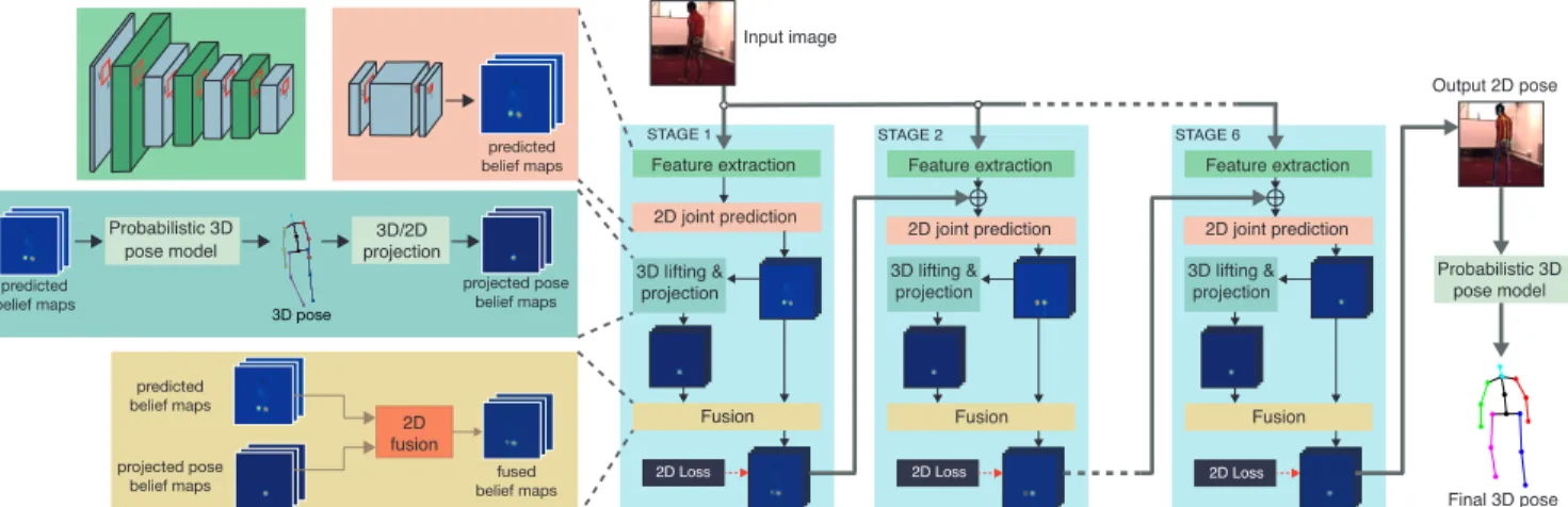
Figure 1:The multistage deep architecture for 2D/3D human pose estimation. Each stage produces as output a set of belief maps for the location of the 2D landmarks (one per landmark). The belief maps from each stage, as well as the image, are used as input to the next stage. Internally, each stage learns to combine: (a)belief maps provided by convolutional 2D joint predictors, with(b)projected pose belief maps, proposed by the probabilistic 3D pose model. The 3D pose layer is responsible for lifting 2D landmark coordinates into 3D and projecting them onto the space of valid 3D poses. These two belief maps are then fused into a single set of output proposals for the 2D landmark locations per stage. The accuracy of the 2D and 3D landmark locations increases progressively through the stages. The loss used at each stage requires only 2D pose annotations, not 3D. The overall architecture is fully differentiable – including the new projected-pose belief maps and 2D-fusion layers – and can be trained end-to-end using back-propagation. [Best viewed in color.]
lifting problem and follow with methods that learn to esti-mate the 3D pose directly from images.
3D pose from known 2D joint positions: A large body of work has focused on recovering the 3D pose of people given perfect 2D joint positions as input. Early approaches
[19,34,25,6] took advantage of anatomical knowledge of
the human skeleton or joint angle limits to recover pose
from a single image. More recent methods [13,28,3] have
focused on learning a prior statistical model of the human body directly from 3D mocap data.
Non-rigid structure from motion approaches (NRSfM)
also recover 3D articulated motion [8, 4, 14, 20] given
known 2D correspondences for the joints in every frame of a monocular video. Their huge advantage, as unsuper-vised methods, is they do not need 3D training data, instead they can learn a linear basis for the 3D poses purely from 2D data. Their main drawback is their need for significant camera movement throughout the sequence to guarantee ac-curate 3D reconstruction. Recent work on NRSfM applied to human pose estimation has focused on escaping these limitations by the use of a linear model to represent shape
variations of the human body. For instance, [10] defined
a generative model based on the assumption that complex shape variations can be decomposed into a mixture of prim-itive shape variations and achieve competprim-itive results.
Representing human 3D pose as a linear combination of a sparse set of 3D bases, pretrained using 3D mocap data, has also proved a popular approach for articulated human motion [28,43,49], while [49] propose a convex relaxation to jointly estimate the coefficients of the sparse
representa-tion and the camera viewpoint [28] and [43] enforce limb
length constraints. Although these approaches can recon-struct 3D pose from a single image, their best results come
from imposing temporal smoothness on the reconstructions of a video sequence.
Recently, Zhao et al. [47] achieved state-of-the-art
re-sults by training a simple neural network to recover 3D pose from known 2D joint positions. Although the results on perfect 2D input data are impressive, the inaccuracies in 2D joint estimation are not modeled and the performance of this approach combined with joint detectors is unknown.
3D pose from images: Most approaches to 3D pose
infer-ence directly from images fall into one of two categories:(i)
models that learn to regress the 3D pose directly from image
features and(ii)pipeline approaches where the 2D pose is
first estimated, typically using discriminatively trained part models or joint predictors, and then lifted into 3D. While regression based methods suffer from the need to annotate all images with ground truth 3D poses – a technically com-plex and elaborate process – for pipeline approaches the challenge is how to account for uncertainty in the measure-ments. Crucial to both types of approaches is the question of how to incorporate the 3D dependencies between the dif-ferent body joints or to leverage other useful 3D geometric information in the inference process.
Many earlier works on human pose estimation from a single image relied on discriminatively trained models to learn a direct mapping from image features such as silhou-ettes, HOG or SIFT, to 3D human poses without passing through 2D landmark estimation [1,12,11,24,32].
Recent direct approaches make use of deep learning [21,
22,40,41]. Regression-based approaches train an
end-to-end network to predict 3D joint locations directly from the image [41,21,22,48]. Liet al. [22] incorporate model joint dependencies in the CNN via a max-margin formalism,
dif-ferentiable kinematic model into the deep learning architec-ture. Tekinet al. [35] propose a deep regression architecture for structured prediction that combines traditional CNNs for supervised learning with an auto-encoder that implicitly en-codes 3D dependencies between body parts.
As CNNs have become more prevalent, 2D joint
estima-tion [44] has become increasingly reliable and many recent
works have looked to exploit this using a pipeline approach.
Papers such as [9,16,40,26] first estimate 2D landmarks
and later 3D spatial relationships are imposed between them using structured learning or graphical models.
Simo-Serra et al. [33] were one of the first to propose
an approach that naturally copes with the noisy detections inherent to off-the-shelf body part detectors by modeling their uncertainty and propagating it through 3D shape space while satisfying geometric and kinematic 3D constraints.
The work [31] also estimates the location of 2D joints
be-fore predicting 3D pose using appearance and the probable 3D pose of discovered parts using a non-parametric model. Another recent example is Bogoet al. [7], who fit a detailed
statistical 3D body model [23] to 2D joint proposals.
Zhouet al. [50] tackles the problem of 3D pose
estima-tion for a monocular image sequence integrating 2D, 3D and temporal information to account for uncertainties in the model and the measurements. Similar to our proposed
ap-proach, Zhouet al.’s method [50] does not need
synchro-nized 2D-3D training data, i.e. it only needs 2D pose
an-notations to train the CNN joint regressor and a separate 3D mocap dataset to learn the 3D sparse basis. Unlike our approach, it relies on temporal smoothness for its best per-formance, and performs poorly on a single image.
Finally, Wuet al. [45]’s 3D Interpreter Network, a recent approach to estimate the skeletal structure of common ob-jects (chairs, sofas, ...) bears similarities with our method. Although our approaches share common ground in the de-coupling of 3D and 2D training data and the use of projec-tion from 3D to improve 2D predicprojec-tions the network archi-tectures are very different and, unlike us, they do not carry out a quantitative evaluation on 3D human pose estimation.
3. Network Architecture
Figure 1 illustrates the main contribution of our
ap-proach, a new multi-stage CNN architecture that can be trained end-to-end to estimate jointly 2D and 3D joint lo-cations. Crucially it includes a novel layer, based on a prob-abilistic 3D model of human pose, responsible for lifting 2D poses into 3D and propagating 3D information about the skeletal structure to the 2D convolutional layers. In this way, the prediction of 2D pose benefits from the 3D
infor-mation encoded. Section4describes the new probabilistic
3D model of human pose, trained on a dataset of 3D
mo-cap data. Section5describes all the new components and
layers of the CNN architecture. Finally, Section6describes
experimental evaluation on the Human3.6M dataset where we obtain state-of-the-art results. In addition we show qual-itative results on images from the MPII and Leeds datasets.
4. Probabilistic 3D Model of Human Pose
One fundamental challenge in creating models of human poses lies in the lack of access to 3D data of sufficient va-riety to characterize the space of human poses. To com-pensate for this lack of data we identify and eliminate con-founding factors such as rotation in the ground plane, limb length, and left-right symmetry that lead to conceptually similar poses being unrecognized in the training data.
Simple preprocessing eliminates some factors. Size vari-ance is addressed by normalizing the data such that the sum of squared limb lengths on the human skeleton is one; while left-right symmetry is exploited by flipping each pose in the x-axis and re-annotating left as right and vice-versa.
4.1. Aligning 3D Human Poses in the Training Set
Allowing for rotational invariance in the ground-plane is more challenging and requires integration with the data model. We seek the optimal rotations for each pose such that after rotating the poses they are closely approximated by a low-rank compact Gaussian distribution.
We formulate this as a problem of optimization over a
set of variables. Given a set ofN training 3D poses, each
represented as a(3×L)matrixPi of 3D landmark
loca-tions, wherei∈ {1,2, .., N}andLis the number of human
joints/landmarks; we seek global estimates of an average
3D pose µ, a set of J orthonormal basis matrices1 eand
noise varianceσ, alongside per sample rotationsRiand
ba-sis coefficientsaito minimize the following estimate
arg min R,µ,a,e,σ N X i=1 ||Pi−Ri(µ+ai·e)||22 (1) + J X j=1 (ai,j·σj)2+ ln J X j=1 σ2 j
Whereai·e=Pjai,jejis the tensor analog of a
mul-tiplication between a vector and a matrix, and|| · ||2
2is the
squared Frobenius norm of the matrix. Here the y-axis is
assumed to point up, and the rotation matricesRi
consid-ered are ground plane rotations. With the large number of 3D pose samples considered (of the order of 1 million when
training on the Human3.6M dataset [15]), and the complex
inter-dependencies between samples foreandσ, the
mem-ory requirements mean that it is not possible to solve di-rectly as a joint optimization over all variables using a non-linear solver such as Ceres. Instead, we carefully initialize
1When we sayeis a set of orthonormal basis matrices we mean that
each matrix, if unwrapped into a vector, is of unit norm and orthogonal to all other unwrapped matrices.
d) c) b) a) g) h) f) e)
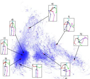
Figure 2: Visualization of the 3D training data after alignment
(see section4.1) using 2D PCA. Notice how all poses have the same orientation.Standing-upposes a), b), c) and d) are all close to each other and far fromsitting-downposes f) and h) which form another clear cluster.
and alternate between performing closed-form PPCA [38]
to updateµ, a,e, σ; and updatingRiusing Ceres [2] to
min-imize the above error. As we do this, we steadily increase the size of the basis from1through to its target sizeJ. This
stops apparent deformations that could be resolved through rotations from becoming locked into the basis at an early stage, and empirically leads to lower cost solutions.
To initialize we use a variant of the Tomasi-Kanade [39]
algorithm to estimate the mean 3D poseµ. As they
com-ponent is not altered by planar rotations, we take as our
es-timate of theycomponent ofµ, the mean of each point in
theydirection. For thexandzcomponents, we interleave
the x andz components of each sample and concatenate
them into a large2N×LmatrixM, and find the rank two
approximation of this such thatM≈A·B. We then
cal-culateAˆby replacing each adjacent pair of rows ofAwith
the closest orthonormal matrix of rank two, and takeAˆ†M
as our estimate2of thexandzcomponents ofµ.
The end result of this optimization is a compact low-rank approximation of the data in which all reconstructed
poses appear to have the same orientation (see Figure2). In
the next section we extend the model to be described as a multi-modal distribution to better capture the variations in the space of 3D human poses.
4.2. A Multi-Modal Model of 3D Human Pose
Although the learned Gaussian model of section4.1can
be directly used to estimate the 3D (see Table 1),
inspec-tion of figure 2 shows that the data is not Gaussian
tributed and is better described using a multiple modal dis-tribution. In doing this, we are heavily inspired both by
approaches such as [27] which characterize the space of
2A†being the pseudo-inverse ofA.
human poses as a mixture of PCA bases, and by related
works such as [42,8] that represent poses as an
interpola-tion between exemplars. These approaches are extremely good at modeling tightly distributed poses (e.g. walking) where samples in the testing data are likely to be close to poses seen in training. This is emphatically not the case in much of the Human3.6M dataset, which we use for
evalu-ation. Zooming in on the edges of Figure2 reveals many
isolated paths where motions occur once and are never re-visited again.
Nonetheless, it is precisely these regions of low-density that we are interested in modeling. As such, we seek a coarse representation of the pose space that says something about the regions of low density but also characterizes the multi-modal nature of the pose space. We represent the data as a mixture of probabilistic PCA models using few
clus-ters, and trained using the EM-algorithm [38]. When using
a small number of clusters, it is important to initialize the algorithm correctly, as accidentally initializing with multi-ple clusters about a single mode, can lead to poor density estimates. To initialize we make use of a simple heuristic.
We first subsample the aligned poses (which we refer to
as P), and then compute the Euclidean distancedamong
pairs. We seek a set ofksamplesSsuch that the distance
between points and their nearest sample is minimized
arg min S X p∈P min s∈S d(s, p) (2)
We findS using greedy selection, holding our previous
es-timate ofSconstant, and iteratively selecting the next
can-didatessuch that{s} ∪Sminimizes the above cost. A
se-lection of 3D pose samples found using this procedure can
be seen in the rendered poses of Figure2. In practice, we
stop proposing candidates when they occur too close to the existing candidates, as shown by samples (a–d), and only choose one candidate from the dominant mode.
Given these candidates for cluster centers, we assign each aligned point to a cluster representing its nearest
can-didate and then run the EM algorithm of [38], building a
mixture of probabilistic PCA bases.
5. A New Convolutional Architecture for 2D
and 3D Pose Inference
Our 3D pose inference from a single RGB image makes use of a multistage deep convolutional architecture, trained end-to-end, that repeatedly fuses and refines 2D and 3D poses, and a second module which takes the final predicted 2D landmarks and lifts them one last time into 3D space for the final estimate (see Figure1).
At its heart, the architecture is a novel refinement of the
Convolutional Pose Machine of Wei et al. [44], who
Stage 1 Stage 2 Stage 3 Stage 4 Stage 5 Stage 6
Stage 1 Stage 2 Stage 3 Stage 4 Stage 5 Stage 6
9.19 mm 7.30 mm 6.64 mm 3.34 mm 3.28 mm 3.10 mm
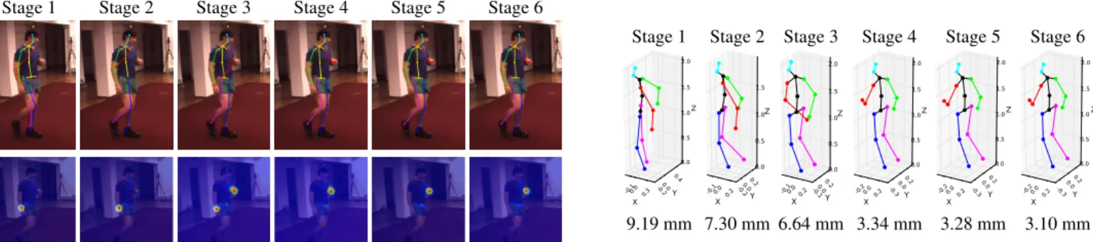
Figure 3: Results returned by different stages of the architecture. Top Left: Evolution of the 2D skeleton after projecting the 3D points back into the 2D space;Bottom Left: Evolution of the beliefs for the landmarkLeft handthrough the stages. Right: 3D skeleton with the relative mean error per landmark in millimeters. Even with incorrect landmark locations, the model returns a physically plausible solution.
iteratively refined 2D pose estimations of landmarks using a mixture of knowledge of the image and of the estimates of landmark locations of the previous stage. We modify this architecture by generating, at each stage, projected 3D pose belief maps which are fused in a learned manner with the standard maps. From an implementation point of view this
is done by introducing two distinct layers, theprobabilistic
3D pose layerand thefusion layer(see Figure1).
Figure 3 shows how the 2D uncertainty in the belief
maps is reduced at each stage of the architecture and how the accuracy of the 3D poses increases with each stage.
5.1. Architecture of each stage
The sequential architecture consists of 6 stages. Each
stage consists of 4 distinct components (see Figure1):
Predicting CNN-based belief-maps: we use a set of con-volutional and pooling layers, equivalent to those used in
the original CPM architecture [44], that combine evidence
obtained from image learned features with the belief maps
obtained from the previous stage (t−1) to predict an
up-dated set of belief maps for the 2D human joint positions.
Lifting 2D belief-maps into 3D:the output of the CNN-based belief maps is taken as input to a new layer that uses
new pretrained probabilistic 3D human pose modelto lift
the proposed 2D poses into 3D.
Projected 2D pose belief maps:The 3D pose estimated by the previous layer is projected back onto the image plane to produce a new set of projected pose belief maps. These maps encapsulate 3D dependencies between the body parts.
2D Fusion layer:The final layer in each stage (described in
section5.5) learns the weights to fuse the two sets of belief
maps into a single estimate passed to the next stage.
Final lifting:The belief maps produced as the output of the
final stage (t = 6) are then lifted into 3D to give the final
estimate for the pose (see Figure1) using our algorithm to
lift 2D poses into 3D.
5.2. Predicting CNN-based belief-maps
Convolutional Pose Machines [44] can be understood as
an updating of the earlier work of Ramakrishnaet al. [29] to use a deep convolutional architecture. In both approaches,
at each stage tand for each landmarkp, the algorithm
re-turns dense per pixel belief mapsbpt[u, v], which show how
confident it is that a joint center or landmark occurs in any
given pixel (u, v). For stages t ∈ {2, . . . , T} the belief
maps are a function of not just the information contained in the image but also the information computed by the previ-ous stage.
In the case of convolutional pose machines, and in our work which uses the same architecture, a summary of the convolution widths and architecture design is shown in Fig-ure1, with more details of training given in [44].
Both [29,44] predict the locations of different landmarks to those captured in the Human3.6M dataset. As such the input and output layers in each stage of the architecture are replaced with a larger set to account for the greater number of landmarks. The new architecture is then initialized by using the weights with those found in CPM’s model for all preexisting layers, with the new layers randomly initialized. After retraining, CPMs return per-pixel estimates of landmark locations, while the techniques for 3D estimation (described in the next section) make use of 2D locations. To transform these belief maps into locations, we select the most confident pixel as the location of each landmark
Yp= arg max
(u,v)
bp[u, v] (3)
5.3. Lifting 2D belief-maps into 3D
We follow [50] in assuming a weak perspective model,
and first describe the simplest case of estimating the 3D pose of a single frame using a unimodal Gaussian 3D pose
model as described in section4. This model is composed
of a mean shapeµ, a set of basis matriceseand variances
Results from the Human3.6M dataset X -0.10.00.1 Y -0.30.00.4 Z 0.0 0.5 1.0 1.5 X -0.10.00.1-0.20.0Y 0.3 Z 0.0 0.5 1.0 1.5 X -0.4 0.0 0.2-0.40.0Y 0.4 Z 0.0 0.5 1.0 1.5 X -0.3 0.00.1-0.3Y 0.00.2 Z 0.0 0.5 1.0 1.5 2.0 X -0.3 0.0 0.2-0.3Y 0.00.4 Z 0.0 0.5 1.0 1.5 2.0 X -0.3 0.00.1-0.20.0Y 0.2 Z 0.0 0.5 1.0 1.5 2.0 X -0.3 0.00.1-0.40.0Y 0.4 Z 0.0 0.5 1.0 1.5 2.0 X -0.20.00.1 Y -0.30.0 0.5 Z 0.0 0.5 1.0 1.5 X -2.2 0.00.6 -0.6 Y 0.0 0.8 Z 0.0 0.5 1.0 1.5 X -0.5 0.0 0.2 -0.5Y 0.00.6 Z 0.0 0.5 1.0 1.5 2.0 X -0.5 0.0 0.2-0.4 Y 0.00.4 Z 0.0 0.5 1.0 1.5 X -1.2 0.0 0.7 Y -0.7 0.0 1.0 Z 0.0 0.5 1.0 1.5 2.0
Success cases from MPII and Leeds
Failure cases from MPII and Leeds
Figure 4:Left:Results from the Human3.6M dataset. The identified 2D landmark positions and 3D skeleton is shown for each pose taken
from different actions: Walking, Phoning, Greeting, Discussion, Sitting Down.Right:Results on images from the MPII [5] (columns 1 to 3) and Leeds [18] datasets (last column). The model was not trained on images as diverse as those contained in these datasets, however it often retrieves correct 2D and 3D joint positions. The last row shows example cases where the method fails either in the identification of 2D or 3D landmarks.
2D Pose refinement in Human3.6M
Figure 5:Landmark refinement:Left: 2D predicted landmark
po-sitions;Right: improved predictions using the projected 3D pose.
from the model that could give rise to a projected image.
arg min
R,a ||
Y −sΠER(µ+a·e)||2
2+||σ·a||22 (4)
WhereΠis the orthographic projection matrix,Ea known
external camera calibration matrix, andsthe estimated
per-frame scale. Although, givenRthis problem is convex in
a ands together3, for an unknown rotation matrixR the
problem is extremely non-convex – even ifais known – and
prone to sticking in local minima using gradient descent. Local optima often lie far apart in pose space and a poor optima leads to a significantly worse 3D reconstructions.
We take advantage of the matrixR’s restricted form that
allows it to be parameterized in terms of a single angleθ.
Rather than attempting to solve this optimization problem
3To see this consider the trivial reparameterization where we solve for
sµ+b·eand then leta=b/s.
using local methods we quantize over the space of possible rotations, and for each choice of rotation, we hold this fixed
and solve forsanda, before picking the minimum cost
so-lution of any choice ofR. With fixed choices of rotation the
termsΠERµandΠERecan be precomputed and finding
the optimalabecomes a simple linear least square problem.
This process is highly efficient and by oversampling the
rotations and exhaustively checking in10,000locations we
can guarantee that a solution extremely close to the global
optima is found. In practice, using20samples and refining
the rotations and basis coefficients of the best found solution using a non-linear least squares solver obtains the same re-construction, and we make use of the faster option of
check-ing80locations and using the best found solution as our 3D
estimate. This puts us close to the global optima and has the same average accuracy as finding the global optima. More-over, it allows us to upgrade from sparse landmark locations to 3D using a single Gaussian at around 3,000 frames a sec-ond using python code on a standard laptop.
To handle models consisting of a mixture of Gaussians,
we follow [27] and simply solve for each Gaussian
indepen-dently and select the most probably solution.
5.4. Projecting 3D poses onto 2D belief maps
Theprojected pose modelis interleaved throughout the
architecture (see Figure1). The goal is to correct the beliefs regarding landmark locations at each stage, by fusing extra information about 3D physical plausibility. Given the
solu-tionR,s, andafrom the previous component, we estimate
a physically plausible projected 3D pose as
ˆ
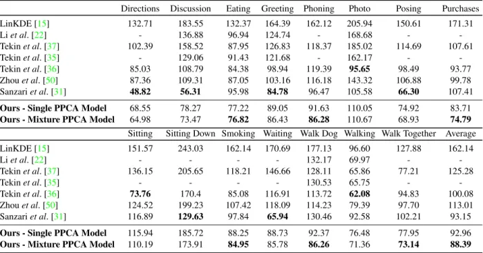
Directions Discussion Eating Greeting Phoning Photo Posing Purchases LinKDE [15] 132.71 183.55 132.37 164.39 162.12 205.94 150.61 171.31 Liet al. [22] - 136.88 96.94 124.74 - 168.68 - -Tekinet al. [37] 102.39 158.52 87.95 126.83 118.37 185.02 114.69 107.61 Tekinet al. [35] - 129.06 91.43 121.68 - 162.17 - -Tekinet al. [36] 85.03 108.79 84.38 98.94 119.39 95.65 98.49 93.77 Zhouet al. [50] 87.36 109.31 87.05 103.16 116.18 143.32 106.88 99.78 Sanzariet al. [31] 48.82 56.31 95.98 84.78 96.47 105.58 66.30 107.41
Ours - Single PPCA Model 68.55 78.27 77.22 89.05 91.63 110.05 74.92 83.71
Ours - Mixture PPCA Model 64.98 73.47 76.82 86.43 86.28 110.67 68.93 74.79
Sitting Sitting Down Smoking Waiting Walk Dog Walking Walk Together Average LinKDE [15] 151.57 243.03 162.14 170.69 177.13 96.60 127.88 162.14 Liet al. [22] - - - - 132.17 69.97 - -Tekinet al. [37] 136.15 205.65 118.21 146.66 128.11 65.86 77.21 125.28 Tekinet al. [35] - - - - 130.53 65.75 - -Tekinet al. [36] 73.76 170.4 85.08 116.91 113.72 62.08 94.83 100.08 Zhouet al. [50] 124.52 199.23 107.42 118.09 114.23 79.39 97.70 113.01 Sanzariet al. [31] 116.89 129.63 97.84 65.94 130.46 92.58 102.21 93.15
Ours - Single PPCA Model 115.94 185.72 88.25 88.73 92.37 76.48 77.95 92.96
Ours - Mixture PPCA Model 110.19 173.91 84.95 85.78 86.26 71.36 73.14 88.39
Table 1: A comparison of the 3D pose estimation results of our approach on the Human3.6M dataset against competitors that follow
Protocol #1for evaluation (3D errors are given in mm). We substantially outperform all other methods in terms of average error showing a 4.7mm average improvement over our closest competitor. Note that some approaches [37,50] use video as input instead of a single frame.
which is then embedded in a belief map as
ˆ bpi,j=
(
1 if(i, j) = ˆYp
0 otherwise. (6)
and then convolved using Gaussian filters.
5.5. 2D Fusion of belief maps
The 2D belief maps predicted by the probabilistic 3D
pose modelare fused with the CNN-based belief mapsbp
according to the following equation
ftp=wt∗bpt+ (1−wt)∗ˆbpt (7)
wherewt∈[0,1]is a weight trained as part of the
end-to-end learning. This set of fused belief mapsftis then passed
to the next stage and used as an input to guide the 2D
re-estimation of joint locations, instead of the belief mapsbt
used by convolutional pose machines.
5.6. The Objective and Training
Following [44], the objective or cost function ct
min-imized at each stage is the the squared distance between
the generated fusion maps of the layerftp, and ground-truth
belief maps bp∗ generated by Gaussian blurring the sparse
ground-truth locations of each landmarkp
ct= L+1 X p=1 X z∈Z ||ftp−bp∗||22 (8)
For end-to-end training the total loss is the sum over all
layers P
t≤6ct. The novel layers were implemented as
an extension of the published code of Convolutional Pose
Machines [44] inside the Caffeframework [17] as Python
layers, with weights updated using Stochastic Gradient De-scent with momentum. Details of the novel gradient updates used lifting estimates through 3d pose space are given in the supplementary materials.
6. Experimental evaluation
Human3.6M dataset: The model was trained and tested on the Human3.6M dataset consisting of 3.6 million
ac-curate 3D human poses [15]. This is a video and mocap
dataset of 5 female and 6 male subjects, captured from 4 dif-ferent viewpoints, that show them performing typical activ-ities (talking on the phone, walking, greeting, eating, etc.).
2D Evaluation:Figure5shows how the 2D predictions are improved by the projected pose model, reducing the over-all mean error per landmark. The 2D error reduction using
our full approach over the estimates of [44] is comparable
in magnitude to the improvement due to the change of
ar-chitecture moving from the work Zhou et al. [50] to the
state-of-the-art 2d architecture [44] (i.e. a reduction of 0.59
pixels vs. 0.81 pixels). See Table2for details.
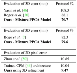
3D Evaluation: Several evaluation protocols have been followed by different authors to measure the performance of their 3D pose estimation methods on the Human3.6M
Evaluation of 3D error (mm) Protocol #2 Yasinet al. [46] 108.3 Rogezet al. [30] 88.1
Ours - Mixture PPCA Model 70.7
Evaluation of 3D error (mm) Protocol #3 Bogoet al. [7] 82.3
Ours - Mixture PPCA Model 79.6
Evaluation of 2D pixel error
Zhouet al. [50] 10.85 Trained CPM [44] architecture 10.04
Oursusing 3D refinement 9.47
Table 2: Further evaluation on the Human3.6M dataset. Top two
tables compare our 3D pose estimation errors against competitors onProtocols #2or#3. Bottom table compares our 2D pose esti-mation error against competitors. Our approach, which lifts the 2D landmark predictions into a plausible 3D model and then projects them back into the image, substantially reduces the error. Note that [50] use video as input and knowledge of the action label.
estimation with previous works, where we take care to eval-uate using the appropriate protocol.
Protocol #1, the most standard evaluation protocol on Human3.6M, was followed by [15,22,37,35,36,50,31]. The training set consists of 5 subjects (S1, S5, S6, S7, S8), while the test set includes 2 subjects (S9, S11). The orig-inal frame rate of 50 FPS is down-sampled to 10 FPS and the evaluation is on sequences coming from all 4 cameras
and all trials. The reported error metric is the3D errori.e.
the Euclidean distance from the estimated 3D joints to the ground truth, averaged over all 17 joints of the Human3.6M
skeletal model. Table 1shows a comparison between our
approach and competing approaches usingProtocol #1. Our
baseline method using a single unimodal probabilistic PCA model outperforms almost every method in most action
types, with the exception of Sanzari et al. [31], which it
still outperforms on average across the entire dataset. The
mixture model improves on this again, offering a4.76mm
improvement over Sanzariet al., our closest competitor.
Protocol #2, followed by [46,30], selects 6 subjects (S1, S5, S6, S7, S8 and S9) for training and subject S11 for testing. The original video is down-sampled to every 64th frame and evaluation is performed on sequences from all 4 cameras and all trials. The error metric reported in this case
is the3D pose errorequivalent to the per-joint 3D error up
to a similarity transformation (i.e. each estimated 3D pose is aligned with the ground truth pose, on a per-frame basis, using Procrustes analysis). The error is averaged over 14
joints. Table2shows a comparison between our approach
and other approaches that useProtocol #2. Although, our
model was trained using only the 5 subjects used for
train-ing inProtocol #1(one fewer subject), it still outperforms
the other methods [30,46].
Protocol #3, followed by [7], selects the same subjects
for training and testing asProtocol #1. However,
evalua-tion is only on sequences captured from the frontal camera (“cam 3”) from trial 1 and the original video is not
sub-sampled. The error metric used in this case is the3D pose
error as described in Protocol #2. The error is averaged
over a subset of 14 joints. Table 2 shows a comparison
between our approach and [7]. Our method outperforms
Bogo et al. [7] by almost 3mm on average, even though
Bogo et al. exploits a high-quality detailed statistical 3D
body model [23] trained on thousands of 3D body scans,
that captures both the variation of human body shape and its deformation through pose.
MPII and Leeds datasets: The proposed approach trained exclusively on the Human3.6M dataset can be used to identify 2D and 3D landmarks of images contained in
different datasets. Figure4 shows some qualitative results
on the MPII dataset [5] and on the Leeds dataset [18],
in-cluding failure cases. Notice how theprobabilistic 3D pose
modelgenerates anatomically plausible poses even though
the 2D landmark estimations are not all correct. However, as shown in bottom row, even small errors in 2D pose can lead to drastically different 3D poses. These inaccuracies could be mitigated without further 3D data by annotating additional RGB images for training from different datasets.
7. Conclusion
We have presented a novel approach to human 3D pose estimation from a single image that outperforms previous solutions. We approach this as a problem of iterative refine-ment in which 3D proposals help refine and improve upon the 2D estimates. Our approach shows the importance of thinking in 3D even for 2D pose estimation within a single image, with our method demonstrating better 2D accuracy
than [44], the 2D approach it is based upon. Our novel
ap-proach for upgrading from 2D to 3D is extremely efficient.
When using 3 models, as in Tables 1 and2, the upgrade
for each stage in CPU-based Python code runs at approx-imately 1,000 frames a second, while a GPU-based real-time approach for Convolutional Pose Machines has been announced. Integrating these systems to provide a reliable real-time 3D pose estimator is a natural future direction, as is integrating this work with a simpler 2D approach for real-time pose estimation on lower power devices.
Acknowledgments
This work was funded by the SecondHands project, from the European Union’s Horizon 2020 Research and Innova-tion programme under grant agreement No 643950. Chris Russell was partially supported by The Alan Turing Insti-tute under EPSRC grant EP/N510129/1.
References
[1] A. Agarwal and B. Triggs. Recovering 3d human pose from monocular images. IEEE transactions on pattern analysis and machine intelligence, 28(1):44–58, 2006.2
[2] S. Agarwal, K. Mierle, and Others. Ceres solver. http: //ceres-solver.org.4
[3] I. Akhter and M. J. Black. Pose-conditioned joint angle lim-its for 3d human pose reconstruction. InProceedings of the IEEE Conference on Computer Vision and Pattern Recogni-tion, pages 1446–1455, 2015.2
[4] I. Akhter, Y. Sheikh, S. Khan, and T. Kanade. Trajectory space: A dual representation for nonrigid structure from mo-tion. IEEE Transactions on Pattern Analysis and Machine Intelligence, 2011.2
[5] M. Andriluka, L. Pishchulin, P. Gehler, and B. Schiele. Hu-man pose estimation: New benchmark and state of the art analysis. InIEEE Conference on Computer Vision and Pat-tern Recognition (CVPR), 2014.6,8
[6] C. Barr´on and I. A. Kakadiaris. Estimating anthropometry and pose from a single uncalibrated image.Computer Vision and Image Understanding, 81(3):269–284, 2001.2
[7] F. Bogo, A. Kanazawa, C. Lassner, P. Gehler, J. Romero, and M. J. Black. Keep it smpl: Automatic estimation of 3d human pose and shape from a single image. InEuropean Conference on Computer Vision, pages 561–578. Springer, 2016.3,8
[8] C. Bregler, A. Hertzmann, and H. Biermann. Recovering non-rigid 3d shape from image streams. InComputer Vision and Pattern Recognition, 2000. Proceedings. IEEE Confer-ence on, volume 2, pages 690–696. IEEE, 2000.2,4
[9] X. Chen and A. L. Yuille. Articulated pose estimation by a graphical model with image dependent pairwise relations. In
Advances in Neural Information Processing Systems, pages 1736–1744, 2014.3
[10] J. Cho, M. Lee, and S. Oh. Complex non-rigid 3d shape recovery using a procrustean normal distribution mix-ture model. International Journal of Computer Vision, 117(3):226–246, 2016.2
[11] C. H. Ek, P. H. S. Torr, and N. D. Lawrence. Gaussian process latent variable models for human pose estimation. In A. Popescu-Belis, S. Renals, and H. Bourlard, editors,
MLMI, volume 4892 ofLecture Notes in Computer Science, pages 132–143. Springer, 2007.2
[12] A. Elgammal and C. Lee. Inferring 3d body pose from sil-houettes using activity manifold learning. InCVPR, 2004.
2
[13] X. Fan, K. Zheng, Y. Zhou, and S. Wang. Pose locality con-strained representation for 3d human pose reconstruction. In
European Conference on Computer Vision, pages 174–188. Springer, 2014.2
[14] P. Gotardo and A. Martinez. Computing smooth time tra-jectories for camera and deformable shape in structure from motion with occlusion.IEEE Transactions on Pattern Anal-ysis and Machine Intelligence, 2011.2
[15] C. Ionescu, D. Papava, V. Olaru, and C. Sminchisescu. Human3. 6m: Large scale datasets and predictive meth-ods for 3d human sensing in natural environments. IEEE
transactions on pattern analysis and machine intelligence, 36(7):1325–1339, 2014.3,7,8
[16] A. Jain, J. Tompson, M. Andriluka, G. W. Taylor, and C. Bre-gler. Learning human pose estimation features with convo-lutional networks.arXiv preprint arXiv:1312.7302, 2013.3
[17] Y. Jia, E. Shelhamer, J. Donahue, S. Karayev, J. Long, R. Gir-shick, S. Guadarrama, and T. Darrell. Caffe: Convolu-tional architecture for fast feature embedding.arXiv preprint arXiv:1408.5093, 2014.7
[18] S. Johnson and M. Everingham. Clustered pose and nonlin-ear appnonlin-earance models for human pose estimation. In Pro-ceedings of the British Machine Vision Conference, 2010. doi:10.5244/C.24.12.6,8
[19] H.-J. Lee and Z. Chen. Determination of 3d human body postures from a single view. Computer Vision, Graphics, and Image Processing, 30(2):148–168, 1985.2
[20] M. Lee, J. Cho, and S. Oh. Procrustean normal distribution for non-rigid structure from motion. IEEE Transactions on Pattern Analysis and Machine Intelligence, 2016.2
[21] S. Li and A. B. Chan. 3d human pose estimation from monocular images with deep convolutional neural network. InAsian Conference on Computer Vision, pages 332–347. Springer, 2014.2
[22] S. Li, W. Zhang, and A. B. Chan. Maximum-margin struc-tured learning with deep networks for 3d human pose estima-tion. InProceedings of the IEEE International Conference on Computer Vision, pages 2848–2856, 2015.2,7,8
[23] M. Loper, N. Mahmood, J. Romero, G. Pons-Moll, and M. J. Black. Smpl: A skinned multi-person linear model. ACM Transactions on Graphics (TOG), 34(6):248, 2015.3,8
[24] G. Mori and J. Malik. Recovering 3d human body configu-rations using shape contexts.PAMI, 2006.2
[25] V. Parameswaran and R. Chellappa. View independent hu-man body pose estimation from a single perspective image. InComputer Vision and Pattern Recognition, 2004. CVPR 2004. Proceedings of the 2004 IEEE Computer Society Con-ference on, volume 2, pages II–16. IEEE, 2004.2
[26] T. Pfister, J. Charles, and A. Zisserman. Flowing convnets for human pose estimation in videos. InProceedings of the IEEE International Conference on Computer Vision, pages 1913–1921, 2015.3
[27] N. Pitelis, C. Russell, and L. Agapito. Learning a mani-fold as an atlas. InComputer Vision and Pattern Recogni-tion (CVPR), 2013 IEEE Conference on, pages 1642–1649. IEEE, 2013.4,6
[28] V. Ramakrishna, T. Kanade, and Y. Sheikh. Reconstructing 3d human pose from 2d image landmarks. InEuropean Con-ference on Computer Vision, pages 573–586. Springer, 2012.
2
[29] V. Ramakrishna, D. Munoz, M. Hebert, J. A. Bagnell, and Y. Sheikh. Pose machines: Articulated pose estimation via inference machines. InEuropean Conference on Computer Vision, pages 33–47. Springer, 2014.5
[30] G. Rogez and C. Schmid. Mocap-guided data augmentation for 3d pose estimation in the wild. InAdvances in Neural Information Processing Systems, pages 3108–3116, 2016.8
[31] M. Sanzari, V. Ntouskos, and F. Pirri. Bayesian image based 3d pose estimation. InEuropean Conference on Computer Vision, pages 566–582. Springer, 2016. 3,7,8
[32] L. Sigal, R. Memisevic, and D. Fleet. Shared kernel infor-mation embedding for discriminative inference. InCVPR, 2009.2
[33] E. Simo-Serra, A. Ramisa, G. Aleny`a, C. Torras, and F. Moreno-Noguer. Single image 3d human pose estima-tion from noisy observaestima-tions. InComputer Vision and Pat-tern Recognition (CVPR), 2012 IEEE Conference on, pages 2673–2680. IEEE, 2012.3
[34] C. J. Taylor. Reconstruction of articulated objects from point correspondences in a single uncalibrated image. In Com-puter Vision and Pattern Recognition, 2000. Proceedings. IEEE Conference on, volume 1, pages 677–684. IEEE, 2000.
2
[35] B. Tekin, I. Katircioglu, M. Salzmann, V. Lepetit, and P. Fua. Structured prediction of 3d human pose with deep neural net-works. InBritish Machine Vision Conference (BMVC), 2016.
3,7,8
[36] B. Tekin, P. M´arquez-Neila, M. Salzmann, and P. Fua. Fus-ing 2d uncertainty and 3d cues for monocular body pose es-timation.arXiv preprint arXiv:1611.05708, 2016.7,8
[37] B. Tekin, X. Sun, X. Wang, V. Lepetit, and P. Fua. Predict-ing people’s 3d poses from short sequences. arXiv preprint arXiv:1504.08200, 2015.7,8
[38] M. E. Tipping and C. M. Bishop. Probabilistic principal component analysis. Journal of the Royal Statistical Soci-ety, Series B, 61:611–622, 1999.4
[39] C. Tomasi and T. Kanade. Shape and motion from image streams under orthography: a factorization method. Inter-national Journal of Computer Vision, 9(2):137–154, 1992.
4
[40] J. J. Tompson, A. Jain, Y. LeCun, and C. Bregler. Joint train-ing of a convolutional network and a graphical model for human pose estimation. InAdvances in neural information processing systems, pages 1799–1807, 2014.2,3
[41] A. Toshev and C. Szegedy. Deeppose: Human pose estima-tion via deep neural networks. InProceedings of the IEEE Conference on Computer Vision and Pattern Recognition, pages 1653–1660, 2014.2
[42] C. Wang, J. Flynn, Y. Wang, and A. L. Yuille. Represent-ing data by a mixture of activated simplices. arXiv preprint arXiv:1412.4102, 2014.4
[43] C. Wang, Y. Wang, Z. Lin, , A. Yuille, and W. Gao. Robust estimation of human poses from a single image. InComputer Vision and Pattern Recognition (CVPR), 2014.2
[44] S.-E. Wei, V. Ramakrishna, T. Kanade, and Y. Sheikh. Con-volutional pose machines.arXiv preprint arXiv:1602.00134, 2016.1,3,4,5,7,8
[45] J. Wu, T. Xue, J. J. Lim, Y. Tian, J. B. Tenenbaum, A. Tor-ralba, and W. T. Freeman. Single image 3d interpreter net-work. InEuropean Conference on Computer Vision, pages 365–382. Springer, 2016.3
[46] H. Yasin, U. Iqbal, B. Kruger, A. Weber, and J. Gall. A dual-source approach for 3d pose estimation from a single image. InIEEE Conference on Computer Vision and Pattern Recognition (CVPR), 2016.8
[47] R. Zhao, Y. Wang, and A. Martinez. A simple, fast and highly-accurate algorithm to recover 3d shape from 2d land-marks on a single image. arXiv preprint arXiv:1609.09058, 2016.2
[48] X. Zhou, X. Sun, W. Zhang, S. Liang, and Y. Wei. Deep kine-matic pose regression. arXiv preprint arXiv:1609.05317, 2016.2
[49] X. Zhou, M. Zhu, S. Leonardos, and K. Daniilidis. Sparse representation for 3d shape estimation: A convex relaxation approach.arXiv preprint arXiv:1509.04309, 2015.2
[50] X. Zhou, M. Zhu, S. Leonardos, K. Derpanis, and K. Dani-ilidis. Sparseness meets deepness: 3d human pose estimation from monocular video. arXiv preprint arXiv:1511.09439, 2015.3,5,7,8
Supplementary Material
1. Computing derivatives for back-propagation through our lifted model
As discussed by the Convolution Pose Machine paper [1] recurrent like architectures such as ours have problems with
vanishing gradientsand for effective training they require an additional loss function to be defined for each layer, that
inde-pendently drives each individual layer to return correct predictions regardless of how this information is used in subsequent layers.
Before we give the derivation of the gradients it should be emphasized that it is entirely possible to train the network without using them – in fact similar results can be obtained by only using the 3D lifting for the forward pass, and not back-propagating the lifting derivatives through the rest of the network. As the additional layers make use of custom Python-based derivatives rather than an efficient implementation, for computational reasons it might preferable to avoid this step. Nonetheless for completeness we include the derivatives.
There are two reasons the gradients are unneeded: Our lifting 3D model we use makes its best predictions when the 2D predictions of the same layer are closest to ground truth, and this is a constraint naturally enforced by the objective of
equation (8) of the main paper. Further, as with Convolutional Pose Machines [1] our architecture suffers from problems with
vanishing gradients. To overcome this Weiet al. [1] defined an objective at each layer, which acted to locally strengthen the
gradients. However, a side effect of this multi-stage objective is that most of the effects of back-propagation happen locally and gradients back-propagated from other layers have little effect on the learning. This makes subtle interactions between layers less influential, and forces the learning process to concentrate on simply making accurate 2D predictions in each layer.
We first give the results for computing the gradients of sparse predicted locationsYˆ fromY (see section 5 of the main
paper), before discussing the gradients induced on the confidence maps by these sparse locations.
1.1. Landmark Gradients
In the interests of readability we neglect the use of indices to indicate stages, the reader should assume that all variables are taken from the same stage. Similarly, when dealing with a mixture of Gaussians, as we are only interested in computing a sub-gradient, the reader should assume that the best model has already been selected in the forward pass and we are computing gradients using only this model.
Recall (section 5 of main body of paper) that the mapping from the initial landmarksY to the projected 3D proposalsYˆ
is given by ˆ Y = ΠR(µ+a·e) (1) where R, a= arg min {R∗∈R,a∗∈RJ}|| Y −ΠR∗(µ+a∗·e)||2 2+ (σ·a∗)2 (2)
whereRis a discrete set of rotations we exhaustively minimize over, andJ is the number of bases ine. Owing to the use
of discrete rotations, this mapping fromY toYˆ is a piecewise smooth approximation of the smooth function defined over a
continiousR, and sub-gradients can be induced by fixingRto its current state. Hence:
dYˆ
da = ΠRe (3)
For the remainder of the section, and to compact notation we will writeEfor the matrix of size2L×J (Lthe number of
landmark points andJ being the number of bases ine) formed by unwrapping tensorΠRe. Similarly, we will unwrap the
2×LmatricesY andYˆ and write them as yandyˆ. We also writepfor the vector representing the unwrapped set of 2D
landmark positionsΠRµ.
We will use[y,0]for the vector formed by vectory followed byJ zeros, and E¯ for the matrix of size (2L+J)×J
formed by concatenatingEwith the matrix that has valuesσalong the diagonals and zero everywhere else. We can rewrite
equation (3) in its new notation as:
dˆy
da=E (4)
and givenR, we can rewrite equation (2) as
a= arg min a∗∈RJ | [y,0]−[p,0]−a∗E¯||2 2 (5) or a= [(y−p),0] ¯E† (6)
withE¯†continuing to represent the pseudo-inverse ofE¯. Hence
da d[y,0]= ¯E † (7) and dˆy dy = dˆy da da dy =EE¯ t (8)
whereE¯tis the truncation ofE¯†.
1.2. Mapping belief gradients to coordinate transform
The coordinates of each predicted landmarkYˆpinduce a Gaussian in the belief mapˆbp. So a change in thexcomponent
ofYˆpinduces an update which is equivalent to a difference of Gaussians.
dˆbp dYˆx p ≈G( ˆYp (x) +δx)−G( ˆYp (x) −δx) 2δx (9)
and the same for theycomponent as well. For computational purposes we takeδxas one pixel. As such, an induced gradient
on the projected belief map near the predicted locationYˆ ˆbpinduces an updating ofYˆ that is propagated through toY using
the sub-gradients described in equation (8).
UpdatingB WritingBfor the the set of allbp, and assumingYpis not in the right location, i.e. given updates∆ ˆB onBˆ
such that ∆ ˆB.dBˆ dYˆ dYˆ dYp 6 = 0,
any update ofbin which we decrease the belief atbpYp and increase anywhere else is a valid sub-gradient. We choose as a
sensible update a negative step atbpof magnitudem=k||∆ ˆB.d
ˆ
B dYˆ
dYˆ
dYp||and a positive update for each elementY of ofBp
of the magnitudem·N(Y, σ2)in the quadrant of a Gaussian of the same width used to generateˆb(i.e.σ= 1see section 5.6
of main paper) and with the same direction as∆ ˆB.dBˆ dYˆ
dYˆ
dYp in eachxandycoordinate.
References
[1] S.-E. Wei, V. Ramakrishna, T. Kanade, and Y. Sheikh. Convolutional pose machines.arXiv preprint arXiv:1602.00134, 2016.1