Discussion Papers
Department of Economics
University of Copenhagen
Studiestræde 6, DK-1455 Copenhagen K., Denmark Tel.: +45 35 32 30 82 – Fax: +45 35 32 30 00
http://www.econ.ku.dk
ISSN: 1601-2461 (online)
No. 08-04
Does Foreign Aid Increase
Foreign Direct Investment?
Pablo Selaya and Eva R. Sunesen
DOES FOREIGN AID INCREASE FOREIGN
DIRECT INVESTMENT?
Pablo Selaya and Eva R. Sunesen
y5 February 2008
Abstract
The notion that foreign aid and foreign direct investment (FDI) are comple-mentary sources of capital is conventional among governments and international cooperation agencies. This paper argues that the notion is incomplete. Within the framework of an open economy Solow model we show that the theoretical relation-ship between foreign aid and FDI is indeterminate. Aid may raise the marginal pro-ductivity of capital by …nancing complementary inputs, such as public infrastructure projects and human capital investment. However, aid may also crowd out produc-tive private investments if it comes in the shape of physical capital transfers. We therefore turn to an empirical analysis of the relationship between FDI and disag-gregated aid ‡ows. Our results strongly support the hypotheses that aid invested in complementary inputs draws in foreign capital while aid invested in physical capi-tal crowds out FDI. The combined e¤ect of these two types of aid is small but on average positive.
Keywords: Foreign aid, foreign direct investment (FDI), open economy Solow
model.
JEL classi…cations: F21, F35, H40, O19.
1
Introduction
A salient point in the UN (2002) Monterrey Report of the International Conference on Fi-nancing for Development is that o¢ cial development assistance (ODA), trade and foreign direct investment (FDI) are three essential tools for development …nancing. In particular:
We are grateful for comments from Carl-Johan Dalgaard, Heino Bohn Nielsen, Finn Tarp, Thomas Rønde, Thomas Barnebeck Andersen and Nina Blöndal, as well as from participants at the DGPE 2007 workshop in Sandbjerg and the Nordic Conference in Development Economics 2007 in Copenhagen.
yDepartment of Economics, University of Copenhagen. Studiestræde 6, 1455 Copenhagen K, Denmark.
"ODA plays an essential role as a complement to other sources of …nancing for development, especially in those countries with the least capacity to at-tract private direct investment. A central challenge, therefore, is to create the necessary domestic and international conditions to facilitate direct investment ‡ows, conducive to achieving national development priorities, to developing countries, particularly Africa, least developed countries, small island develop-ing States, and landlocked developdevelop-ing countries, and also to countries with economies in transition." (UN, 2002, p. 9).
However, the implicit presumption that ODA has a "catalysing" e¤ect on FDI, i.e., that aid and FDI are complements, is by no means evident. Kosack and Tobin (2006) argue that aid and FDI are unrelated, because aid is mainly oriented to support the government budget and …nance investments in human capital, while FDI is a private sector decision and relatively more connected to physical capital. Caselli and Feyrer (2007) …nd that the marginal product of capital (MPK) is roughly the same across countries, and one of the implications is that increasing aid in‡ows to developing countries will lower the MPK in these economies and will tend to be fully o¤set by out‡ows of other types of capital investments (p. 540). If this is the case, aid and FDI are clearly closer to being substitutes rather than being complements.
This paper provides a uni…ed framework for assessing the relative merit of these dif-ferent claims. We set up an open-economy Solow model with perfect capital mobility that distinguishes between aid directed towards complementary factors of production and aid invested in physical capital. The distinction serves to illustrate, on the one hand, that aid invested in complementary factors increases MPK in the recipient country, which tends to draw in additional foreign resources, and thus helps to sustain a higher level of capital over time. For example, aid can ease important bottlenecks in poor countries by …nancing public infrastructure and human capital investments that would not have been undertaken private actors (due to the free-riding problem in …nancing public goods), nor by public agents (because of the budgetary constraints that prevent aid-recipient govern-ments from undertaking this type of investgovern-ments). On the other hand, the model also shows that foreign aid invested in physical capital directly competes with other types of capital, and thus replaces investments that private actors would have undertaken anyway. In this case, capital mobility and rate-of-return equalisation across countries will give rise to a ‡ight of other types of capital after an aid ‡ow has been received.
The theoretical model provides a number of results and testable predictions. First, for a given level of domestic saving, aid invested in physical capital crowds out other types of foreign investments in physical capital, one for one. Second, aid invested in complementary factors of production has an ambiguous e¤ect on FDI. The logic of the ambiguity is that, while an increase in complementary factors increases MPK, the productivity increase also raises income, domestic savings and domestic investments, which tends to lower MPK
and thus to crowd out foreign investments. These two …ndings suggest that the overall impact of aid on FDI is ambiguous and that the composition of aid matters. Finally, the relationship between complementary aid and FDI is unlikely to be linear, so scale e¤ects from this type of aid should be taken into account.
We take the implications of our theoretical model to the data utilising a panel of 84 countries over the period 1970-2001. We …nd a large and positive e¤ect of aid invested in complementary factors, while aid invested in physical capital has a negative impact on FDI. Although the combined impact of these two types of aid on FDI remains positive, our results imply that more aid should be directed towards inputs complementary to physical capital to optimise the return on aid. The results are robust to (1) a broader de…nition of complementary aid than that adopted in our benchmark estimations, (2) to allowing for imperfect capital mobility, and (3) to including other traditional FDI determinants.
The paper is structured as follows. Section 2 reviews the scarce empirical literature on FDI and aid. Section 3 introduces the theoretical model of FDI and aid building on an open economy Solow model with perfect capital mobility. Section 4 discusses relevant econometric issues and presents the data. Section 5 shows the results, and Section 6 tests their robustness. Section 7 sums up and discusses policy implications.
2
Literature Review
The relationship between aid and FDI is controversial and empirical results remain incon-clusive. To our knowledge, only four papers explicitly analyse the relationship between aid and FDI. Harms and Lutz (2006) and Karakaplan et al. (2005) analyse the question for a broad sample of developing countries. Karakaplan et al. (2005) …nd that aid has a negative direct e¤ect on FDI and that both good governance and …nancial market devel-opment signi…cantly improve the impact of aid on subsequent ‡ows of FDI. Harms and Lutz (2006), on the other hand, …nd that once they control for the regulatory burden in the host country, aid works as a complement to FDI and, surprisingly, that the catalysing e¤ect of foreign aid is stronger in countries that are characterised by an unfavourable institutional environment.
The two case studies based on Japanese FDI and aid ‡ows in Kimura and Todo (2007) and Blaise (2005) also …nd incongruent results. While Blaise (2005) …nds positive e¤ects of aid to infrastructure projects, Kimura and Todo (2007) …nd no positive infrastructure e¤ect, no negative rent-seeking e¤ect but a positive vanguard e¤ect (arising when foreign aid from a particular donor country promotes FDI from the same country but not from other countries).
This paper argues that the mixed results can be explained by the high level of ag-gregation of the aid variable. While Karakaplan et al. (2005) include only overall ODA, Harms and Lutz (2006) also distinguish between grants, technical cooperation grants, as
well as bilateral and multilateral aid. However, it remains unclear why one would expect foreign investors to react di¤erently to these sources of aid. Kimura and Todo (2007) apply the idea of di¤erent types of aid, but construct their proxies relying only on data for aid commitments and they only separate out aid to physical infrastructure.
3
A Theoretical Model of FDI and Aid
A general shortcoming in the empirical literature is the lack of consensus on the speci…-cation of the FDI relation, and none of the existing empirical papers on aid and FDI are supported by a theoretical model. This paper closes this gap by proposing a Solow model for a small open economy to model the main characteristics of the relationship between aid and FDI.1
We assume a Cobb-Douglas production function where GDP per capita,y, is given by
y=Ak , (1)
wherek is the stock of physical capital per capita, K
L, is a constant andA denotes total
factor productivity.
We assume that the total ‡ow of foreign aid, AID, can be split into aid invested in complementary factors,AIDA, and aid invested in physical capital, AIDK, whereAID=
AIDA+AIDK. AIDAby nature raises the marginal productivity of all production factors
that are complementary to physical capital.2 For example, infrastructure investments lead
to the interconnection of markets (Easterly and Levine, 1999), while investments in human capital improve technology adoption. AIDK, on the other hand, enters the production
function only through its e¤ect on physical capital accumulation, and has no (augmenting) e¤ect on total factor productivity.3
To model this explicitly, we …rst assume that complementary aid has an augmenting e¤ect on all production factors that are complementary to physical capital, and we thus allow the ‡ow of AIDA to increase the existing stock (A0) of A in the economy:
A=A0+AIDA. (2)
Allowing complementary aid to have a direct impact onA is a shorthand for the idea that
AIDAhas an augmenting e¤ect on any production factor other thank(e.g. human capital,
1One exception is Beladi and Oladi (2007) who analyse the question in a general equilibrium setting
where all foreign aid is used to …nance public goods.
2The argument of complementarity between public and private investment is generalised by
Clar-ida (1993) and Chatterjee et al. (2003). Reinikka and Svensson (2002) …nd empirical support for the importance of complementary public capital for foreign investors.
3We thus allow part of foreign aid to be productivity enhancing while FDI brings no spillovers. In
reality, all capital transfers might contain some knowledge transfer but the assumption is made to keep the model simple and tractable.
public investments, new technology, etc.) and, thus, it is able to increase –ultimately– the MPK.
Second, we assume an open economy.4 Accordingly, in per capita terms, capital
equip-ment can be …nanced by (i) domestic savings (S =sy, where s is a given savings rate), (ii) foreign direct investments (f di) and (iii) the in‡ow of aid invested in physical capital (aidK). Then capital accumulation per capita is given by
_
k =sy+f di+aidK (n+ )k, (3)
where n is the population growth rate and is a …xed depreciation rate.
With perfect capital mobility, the world real rate of return,rw, pins down at any point
in time the net return to capital (MPK ), and thus
rw =MPK =A k 1 . (4)
According to (4), the steady state level ofk at any point in time is given by
k = A
r
1 1
, (5)
where r is de…ned as a gross world real rate of return, rw+ .
Rewriting (3) taking (5) as given, the ‡ow of FDI per capita is determined as the residual
f di= aidK sy + (n+ )k , (6)
where y =Ak .
At a …rst glance, (6) seems to support the Caselli and Feyrer (2007) conjecture that aid and FDI are substitutes: for a given level of domestic savings, equalisation between MPK and r requires an increase in foreign aid to be accommodated by a proportional reduction in FDI:
@f di @aidK
= 1. (7)
However, this …nding only holds for aid invested in physical capital. The e¤ect of complementary aid, on the other hand, has two components:
@f di @aidA = s @y @aidA + (n+ ) @k @aidA . (8) First, since s @y @aidA =s@(Ak ) @aidA =s Lk +A k 1 @k @aidA >0, (9)
complementary aid has a positive e¤ect on domestic savings and thus on domestically …nanced capital investments. This result comes from the fact that aidA shifts the
pro-duction function thereby raising the steady state levels of income and domestic savings. Given the assumption of MPK equalisation in (4), the corresponding increase in domesti-cally …nanced investments causes a proportional reduction in the need for FDI of the size
s@aid@y A. Also, since @k @aidA = @ @aidA A r 1 1 ! = 1 1 A r 1 L r >0, (10)
we see that complementary aid has a positive e¤ect on the steady state capital stock. This …nding is based on the augmenting e¤ect of aidA, which raises MPK and thus allows
the recipient country to increase its capital stock without experiencing a counterbalancing capital ‡ight. That is, for a …xed s, aid-…nanced investments in complementary factors allow a sustainable increase in FDI equal to (n+ )@aid@k
A.
This model holds then several implications that should be taken into account when assessing the empirical relationship between aid and FDI. First, the e¤ect of total aid on FDI is ambiguous: @f di @aid = @f di @aidK + @f di @aidA = 1 s @y @aidA + (n+ ) @k @aidA ? 0, (11)
because we expect aid to production sectors to have a negative e¤ect on FDI, but the e¤ect of complementary aid is indeterminate. Second, from equations (9) and (10), since the marginal e¤ect of complementary aid on FDI includes the level of aid itself, the relationship between complementary aid and FDI is not linear. In particular, there are scale e¤ects from complementary aid that should be taken into account. Since s@aid@y
A
and (n+ )@aid@k
A work in opposite directions, the sign of the second order e¤ects will also
be indeterminate and will need to be assessed empirically. Third, the model stresses the need to take all sources of capital into account, and it is therefore essential to include domestic savings as an additional explanatory variable in the empirical FDI analysis. To our knowledge, this has not been done before.
4
Econometric Issues
In a panel setting, the econometric interpretation of the aid-FDI relationship is
f diit = 0+ 1A 0 it+ 2nit+ 3Sit+ 4aid K it + 5aid A it+ 6 aid A it 2 +uit, (12)
where f diit is FDI per capita in country iduring period t, A0it is the overall productivity
level at the beginning of period t, nit is population growth, Sit is domestic savings per
capita, aidK
it is aid invested in physical capital, and aidAit is aid invested in
complemen-tary factors. The square of aidA
it is included in (12) to control for the scale e¤ects of
complementary aid.
We expect 1 to be positive since a high productivity level gives a high steady state level of capital, 2 should be positive since a fast growing population lowers the per capita
capital stock and thus allows for an increase in FDI per capita, and 3 should be negative
since high domestic saving lowers the need for foreign capital. From equation (7) we know that aidK crowds out foreign investments one-to-one, 4 = 1, whereas the e¤ect ofaidA
( 5 and 6) is indeterminate. Since data on total productivity is unavailable, the next section will discuss the strategy used to identify A0
it empirically.
4.1
Productivity
Since data on the initial productivity level (A0
it) is unavailable, we need to …nd valid
proxies. In the …rst case, we use pooled OLS (POLS) and estimate
f diit = t+ 0+ 1nit+ 2Sit+ 3aid K it + 4aid A it+ 5 aid A it 2 +uit, (13)
where t is a time-speci…c constant that captures common productivity shocks at timet.
However, not all countries start out with the same initial conditions and we thus allow also for cross sectional di¤erences in productivity by including time-invariant country-speci…c …xed e¤ects, i, f diit = t+ i+ 0+ 1nit+ 2Sit+ 3aid K it + 4aid A it+ 5 aid A it 2 +uit. (14)
This equation can be estimated consistently and e¢ ciently with a …xed e¤ects model (FE). However, if productivity evolves unequally across countries over time, regression (14) leaves out important information. We therefore extend the list of variables to include a lagged dependent variable, which captures time-moving country-speci…c factors as well as agglomeration e¤ects, f diit = t+ i+ 0+ 1f diit 1+ 2nit+ 3Sit+ 4aid K it + 5aid A it+ 6 aid A it 2 +uit. (15)
Equation (15) can be estimated consistently and e¢ ciently using the Arellano and Bond (1991) Generalised Method of Moments (GMM) estimator. It is important to notice that including a lagged dependent variable also reduces the need to control for other FDI determinants. All estimators use standard errors that are robust to arbitrary heteroskedasticity as well as intra-group correlation (clustering).
4.2
Endogeneity
We need to consider the possible endogeneity of aid in estimating the above equations, since all estimators are consistent only if all explanatory variables are exogenous. Aid would be endogenous, for example, if donors systematically disburse more resources to those countries that are neglected by private foreign investors (Harms and Lutz, 2006). We therefore estimate (13)–(15) following the instrumentation strategy in Hansen and Tarp (2000, 2001), Dalgaard and Hansen (2001) and Dalgaard et al. (2004).
The …rst set of instruments accounts for donors’overall preference for granting more aid to countries with smaller populations and lower levels of income per capita and thus includes (lagged) interactions between levels of aid and (i) the size of population and (ii) the initial level of GDP per capita in the recipient country. We also include the lagged level of aid to account for persistency in other determinants of aid as well as a dummy variable for African countries in the CFA franc zone to capture particular donors’strategic interests.
Tests con…rm the validity of our instruments, and the Durbin-Wu-Hausman test …nds that the aid variables should be treated as endogenous in the FDI relation. All the results reported in the next section are therefore based on Instrumental Variables (IV) methods.
4.3
Data
The dependent variable,f diit, is net FDI in‡ows in constant US dollars from the UNCTAD
Foreign Direct Investment database, divided by the population to control for country size. The main explanatory variables are the population growth rate and savings per capita from the WDI (2005).
The aid variables are based on total net ‡ows of o¢ cial aid disbursements reported in the OECD/DAC database. Since data on sectoral disbursements are available only after 1990, the measure of per capita aid ‡ows to sector s, aidsit, is constructed using sectoral commitments as a proxy for sectoral disbursements. In particular, we follow Clemens et al. (2004) and Thiele et al. (2006) and assume that the proportion of aid actually disbursed to sector s is equal to the proportion of aid committed to sector s, and hence that aidsit commit s it P scommit s it P said s it, (16)
where commitsit is the amount of ODA commitments to sectors. Approximating sectoral disbursements with sectoral commitments may cause some concerns due to di¤erences in de…nitions and statistical record (see Clemens et al., 2004, for more details). However, according to Odedokun (2003) and Clemens et al. (2004) this problem is likely to be small since disbursements and commitments (both on the aggregate and sectoral levels) are highly correlated. Also, annual discrepancies are likely to be larger than averages,
and we thus average the data over …ve-year intervals.
Aid is decomposed into two broad categories according to its purpose of investment: Aid invested in complementary inputs: aid oriented to social infrastructure (such as education, health, and water supply projects) and economic infrastructure (such as energy, transportation and communications projects).
Aid invested in physical capital: contributions to directly productive sectors (such as agriculture, manufacturing, trade, banking and tourism projects).
These two aid categories capture the main characteristics of aidA and aidK: aid
in-vested in complementary factors is intended to generate positive spillover e¤ects (public goods, inputs complementary to physical capital) whereas aid invested in physical capi-tal has a more narrow purpose and could more easily have been undertaken by private investors. Other sectoral aid categories (like multisector support, programme assistance, debt reorganisation, emergency assistance and unallocated types of aid) are excluded from the analysis since they are primarily oriented to provide …scal budget support in the recipient country.5
5
Results
Figure 1 in Appendix shows the partial correlation between FDI and aid invested in physical capital. While there seems to be a negative relationship between the two vari-ables, it is di¢ cult to assess if there is full crowding out from the downwards sloping line (that is, to assess if the slope is 1). Figure 2 in Appendix depicts the partial correla-tion between FDI and aid invested in complementary goods. The …gure clearly indicates that the two variables are positively correlated and that the relationship might not be linear. However, the exact predictions from the theoretical model can only be tested in a more comprehensive framework where country-speci…c characteristics capture the cross-sectional heteroskedasticity clearly prevalent in the …gures.
Results from estimating equations (13)–(15) for a sample of 84 countries using …ve-year intervals are reported in Table 1. Independently of the chosen estimator, our results strongly support the notion that aid invested in complementary factors has a catalysing e¤ect on FDI. This means that the short-run replacement e¤ect of aidA on FDI is
out-weighed by the positive e¤ect that complementary aid has on the long-run levels of income and capital per capita. A Hausman test con…rms the signi…cance of …xed e¤ects, and the highly signi…cant lagged dependent variable suggests that we should rely on the consistent
5Section 6 includes a test for robusteness of the results with respect to the de…nition of complementary
aid, and a note about the changes in the results when variables possibly correlated withaidAare included
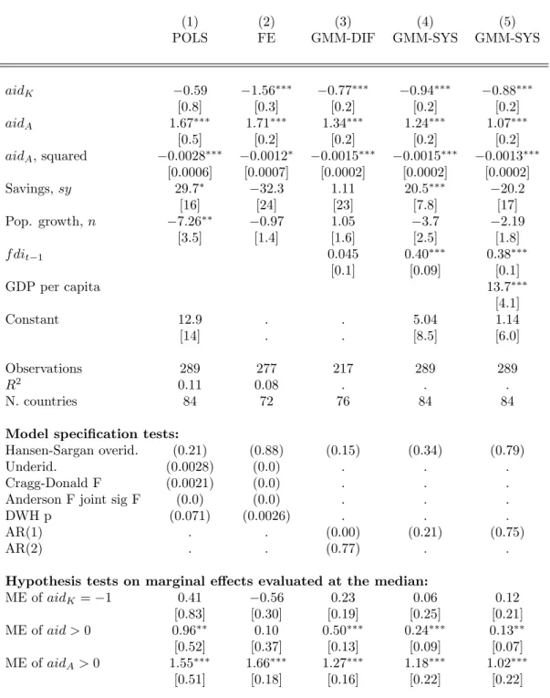
Table 1: FDI and Foreign Aid
(1) (2) (3) (4) (5)
POLS FE GMM-DIF GMM-SYS GMM-SYS
aidK 0:59 1:56 0:77 0:94 0:88 [0:8] [0:3] [0:2] [0:2] [0:2] aidA 1:67 1:71 1:34 1:24 1:07 [0:5] [0:2] [0:2] [0:2] [0:2] aidA, squared 0:0028 0:0012 0:0015 0:0015 0:0013 [0:0006] [0:0007] [0:0002] [0:0002] [0:0002] Savings,sy 29:7 32:3 1:11 20:5 20:2 [16] [24] [23] [7:8] [17] Pop. growth,n 7:26 0:97 1:05 3:7 2:19 [3:5] [1:4] [1:6] [2:5] [1:8] f dit 1 0:045 0:40 0:38 [0:1] [0:09] [0:1] GDP per capita 13:7 [4:1] Constant 12:9 : : 5:04 1:14 [14] : : [8:5] [6:0] Observations 289 277 217 289 289 R2 0:11 0:08 : : : N. countries 84 72 76 84 84
Model speci…cation tests:
Hansen-Sargan overid. (0:21) (0:88) (0:15) (0:34) (0:79)
Underid. (0:0028) (0:0) : : :
Cragg-Donald F (0:0021) (0:0) : : :
Anderson F joint sig F (0:0) (0:0) : : :
DWH p (0:071) (0:0026) : : :
AR(1) : : (0:00) (0:21) (0:75)
AR(2) : : (0:77) : :
Hypothesis tests on marginal e¤ects evaluated at the median:
ME ofaidK = 1 0:41 0:56 0:23 0:06 0:12 [0:83] [0:30] [0:19] [0:25] [0:21] ME ofaid >0 0:96 0:10 0:50 0:24 0:13 [0:52] [0:37] [0:13] [0:09] [0:07] ME ofaidA>0 1:55 1:66 1:27 1:18 1:02 [0:51] [0:18] [0:16] [0:22] [0:22]
Notes. *** p<0.01, ** p<0.05, * p<0.1. Robust standard errors in brackets, p-values in parentheses. The dependent variable is FDI per capita. All regressions include time dummies. Aid variables are instrumented with own lags, interactions with GDP per capita, log(pop) and a FRZ dummy.
and e¢ cient Arellano and Bond (1991) GMM estimator in our further analysis. When the time series are persistent, the …rst-di¤erence GMM (GMM-DIF) estimator is poorly behaved since under such conditions lagged levels of the variables are only weak instru-ments for subsequent …rst-di¤erences. We therefore rely on the system GMM (GMM-SYS) estimator suggested by Arellano and Bover (1995) and Blundell and Bond (1998). All variables are treated as endogenous, which means that instruments should be lagged two periods or more to be valid.
The results in column (4) in Table 1 show that, for a given domestic savings rate, one aid dollar invested in complementary factors draws in 1.24 dollars of FDI, both in per capita terms. The square of complementary aid is negative and signi…cant, suggesting that the "savings" e¤ect described in equation (9) dominates for su¢ ciently high levels of
aidA. Evaluated at the median of the sample, our results indicate that the marginal e¤ect
of aidA on f di is 1.18, and a Wald test con…rms it to be signi…cantly positive. Having
speci…ed a dynamic model, we can calculate the long run e¤ect of aidA by assuming a
that the level of FDI per capita is the same in every period. Evaluating at the median, we …nd that one additional aid dollar per capita invested in complementary factors draws in 1.97 (1.18/0.6) dollars of FDI per capita in the long run. We conclude from this that
aidA generates important short run as well as long run bene…ts for foreign investors.
The results also con…rm the crowding out e¤ect of aid invested in physical capital, since one aid dollar per capita invested in physical capital replaces 0.94 dollars of f di, which accumulate to 1.57 dollars in the long run (0.94/0.6).
The e¤ect of population growth is insigni…cant throughout the analysis. But, con-trary to the prediction from our model, we …nd a positive rather than a negative e¤ect of domestic savings on f di. A plausible explanation is that foreign investors look explicitly at data on national savings when making their investment decisions and interpret a high
s as a signal of sustained growth history and good economic prospects.6 To adjust for
this positive externality we include GDP per capita in column (5). Adjusting for the pur-chasing power of the population leaves savings insigni…cant and negative, which suggest that once we correct for the positive signalling e¤ect of a high saving rate, domestic and foreign capital are substitutes as suggested by the theoretical model.
Finally, we perform some tests of hypothesis and present the results at the bottom of the Table. We test the Caselli and Feyrer (2007) conjecture that aid invested in physical capital replaces FDI one for one. The Wald tests show that we cannot reject its validity in most of the cases. We also …nd that the combined e¤ect of aidA and aidK is signi…cantly
positive and between 0.21 and 0.24 (evaluated at the median of the sample), which implies that the substitution e¤ect ofaidK is more than outweighed by the positive e¤ects ofaidA
6This is in line with evidence showing that the households with the highest lifetime incomes are the
ones with highest lifetime saving rates (Carroll, 2000), and that higher growth rates lead to higher savings rates (Carroll, Overland and Weil, 2000; Loayza, Schmidt-Hebbel and Servén, 2000).
on f di in a typical country. If the marginal e¤ects are evaluated at the mean instead of the median, our conclusions remain the same.
6
Robustness
In light of the important policy implications arising from our results, it is necessary to ensure that these results are robust to correcting for possible misspeci…cations in the empirical relationship between FDI and aid. We carry out three basic checks for robustness of our empirical …ndings.
6.1
Technical Assistance
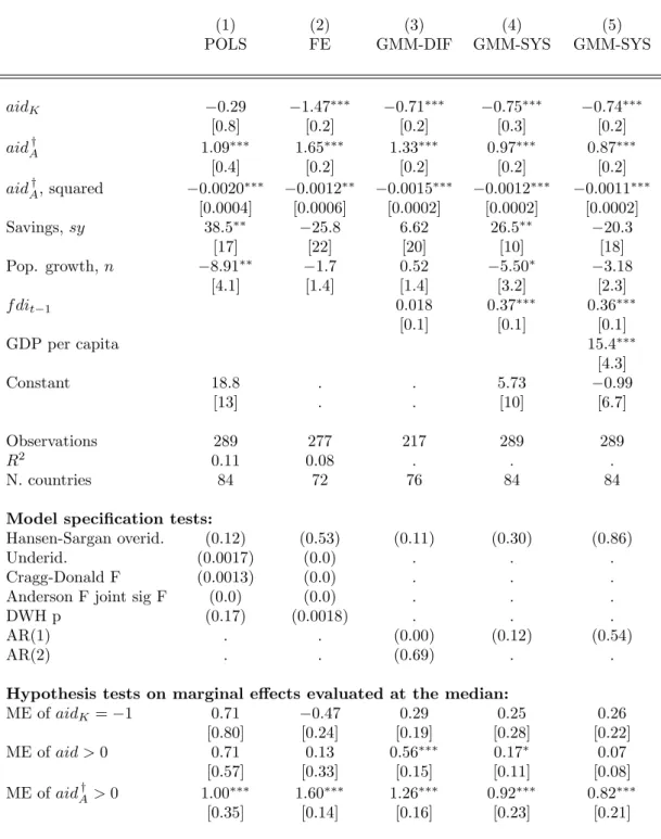
The grouping of aid variables could be questioned. In particular, aid in this paper does not include Technical Cooperation Grants (TCGs), which contribute to development primarily through education and training. Since TCGs consist of activities involving the supply of human resources or actions targeted on human resources (education, training, and advice) one could easily argue that TCGs would have the same impact as aid invested in complementary factors. In the Appendix (Table 4) we therefore replicate the speci…cations from Table 1 using an extended de…nition ofaidAthat includes also TCGs from the OECD
database. Although there is a slight drop in the size of the coe¢ cients, the results from Table 1 carry over.
6.2
Imperfect Capital Mobility
If mobility of capital is imperfect, MPK should be allowed to deviate from the gross world interest rate by a risk-premium, , that re‡ects idiosyncratic country characteristics. In this case, the …rst-order condition in (4) should read
r+ =MPK, (17)
and the capital stock in (5) should be rede…ned accordingly:
k = A
r+
1 1
. (18)
While this renders the e¤ect of aid invested in physical capital unchanged, the e¤ect of complementary aid becomes somewhat more complicated. The risk premium impact FDI directly through (18) but, given that
@k @aidA = @ @aidA A r+ 1 1 ! = 1 1 A r+ 1 L r+ , (19)
the marginal e¤ect of aidA will also depend on the risk premium and thus on
country-speci…c characteristics. To capture this econometrically, we include the risk premium level and its interaction with aidA, and estimate
f diit = t+ i+ 0+ 1nit+ 2Sit+ 3aid K it + 4aid A it+ 5 aid A it 2 (20) + 6 it+ 7 aidAit it +uit.
6 and 7 are expected to be negative because higher risk reduces countryi’s
attrac-tiveness as an investment location.
To capture the risk premium we include the overall International Country Risk Guide rating as well as its three subcategories of risk: political, …nancial and economic.7 All risk variables are treated as endogenous. In general, lower political risk is associated with higher levels of overall accountability, stability and institutional quality in the political process. In particular, from the ICRG rankings, political risk is lower (1) the higher the government stability, (2) the better the socioeconomic conditions and the investment pro…le, (3) the lower the number of internal con‡icts, external con‡icts and political corruption, (4) the lower the military is involved in politics, (5) the lower the religious and the ethnic tensions, (6) the higher the prevalence of law and order, and (7) the larger the degrees of democratic accountability and bureaucratic quality. Results from estimating (20) including these political risk measures are reported in Table 2.8
The political risk variable enters only signi…cantly in four cases. Relative absence of external con‡ict, low level of religious tensions and a high level of democratic account-ability suggest all a lower risk premium and tend to attract foreign investors. However, the prevalence of law and order shows a negative impact on FDI in‡ows (signi…cant only at the 10% level, though). This counter intuitive result might be due to the fact that we have already accounted for domestic savings, which will be highly correlated with this risk variable: countries characterised by law and order tend to have higher domestic saving.
The interactions between complementary aid and the political risk indicator are more often signi…cant, and the results suggest that government stability, favourable socioeco-nomic conditions, an attractive investment pro…le, low military interference in politics and better bureaucratic quality are all supportive of a high steady-state level of capital. Although the results shows a negative impact of the interaction between aidA and the
index for low degree of religious tensions, the net marginal e¤ect on FDI remains positive. Table 3 presents similar estimations taking into account di¤erent economic and …nan-cial risk measures. The economic risk variables re‡ect the macroeconomic situation and
7In order to detect signi…cant e¤ects of aid on FDI, Karakaplan et al. (2005) and Harms and Lutz
(2006) use aid interacted with the Kaufmann et al. (2005) governance indicators to capture di¤erences in government e¤ectiveness.
8For the results in Table 2, a high value of the di¤erent political-risk measures is associated a low
overall political risk, and hence, a high value of the di¤erent risk measures should have a positive e¤ect onf di.
T a b le 2 : F D I a n d F o re ig n A id — P o li ti ca l R is k P oli tical r is k Risk ICR G G o vt. So cio-e c. In v estm. In ternal Exter n al P oli tical Mil itar y Re ligio u s La w a n d Ethn ic D emo c. Bureau c. meas ure: inde x stab . cond it. p ro… le con‡ ic t con‡ ic t cor rup t. in p ol itics te nsions O rder tens ion s acc o u n t. q u al it y (1) (2) (3) (4) (5) (6) (7) (8) (9 ) (10) (11) (12) (13) ai dK 0 : 78 0 : 69 0 : 80 0 : 68 0 : 99 0 : 96 0 : 92 0 : 65 0 : 96 1 : 00 0 : 98 0 : 87 0 : 71 [0 : 3] [0 : 3] [0 : 2] [0 : 3] [0 : 2] [0 : 3] [0 : 3] [0 : 3] [0 : 2] [0 : 2] [0 : 3] [0 : 3] [0 : 3] ai dA 0 : 34 0 : 48 0 : 41 0 : 36 1 : 32 1 : 30 1 : 06 0 : 71 1 : 57 1 : 24 1 : 55 1 : 14 0 : 92 [0 : 7] [0 : 6] [0 : 2] [0 : 5] [0 : 2] [0 : 5] [0 : 6] [0 : 4] [0 : 2] [0 : 4] [0 : 3] [0 : 3] [0 : 4] ai dA , squared 0 : 0016 0 : 0015 0 : 0016 0 : 0015 0 : 0016 0 : 0015 0 : 0014 0 : 0015 0 : 0014 0 : 0016 0 : 0015 0 : 0014 0 : 0015 [0 : 0002] [0 : 0002] [0 : 0002] [0 : 0002] [0 : 0003] [0 : 0002] [0 : 0003] [0 : 0002] [0 : 0002] [0 : 0002] [0 : 0002] [0 : 0002] [0 : 0002] ai dA Risk 0 : 014 0 : 094 0 : 13 0 : 11 0 : 00088 0 : 0025 0 : 062 0 : 13 0 : 083 0 : 038 0 : 056 0 : 013 0 : 14 [0 : 009] [0 : 04] [0 : 02] [0 : 04] [0 : 03] [0 : 04] [0 : 2] [0 : 06] [0 : 02] [0 : 09] [0 : 05] [0 : 05] [0 : 06] Risk 0 : 1 4 : 56 0 : 6 0 : 6 2 : 01 4 : 77 0 : 83 4 : 59 5 : 94 10 : 9 0 : 8 8 : 58 4 : 21 [0 : 6] [4 : 0] [3 : 3] [3 : 6] [1 : 9] [2 : 6] [7 : 0] [3 : 5] [3 : 1] [5 : 7] [3 : 6] [4 : 2] [4 : 5] f d it 1 0 : 41 0 : 41 0 : 41 0 : 43 0 : 43 0 : 42 0 : 40 0 : 45 0 : 39 0 : 43 0 : 42 0 : 42 0 : 39 [0 : 10] [0 : 09] [0 : 10] [0 : 09] [0 : 09] [0 : 09] [0 : 1] [0 : 10] [0 : 1] [0 : 10] [0 : 10] [0 : 1] [0 : 09] Sa v ings, sy 16 : 3 21 : 7 21 : 2 20 : 4 24 : 0 18 : 2 22 : 0 19 : 5 26 : 0 26 : 7 22 : 1 21 : 2 22 : 2 [8 : 2] [7 : 9] [10] [7 : 4] [7 : 8] [8 : 0] [8 : 9] [7 : 9] [8 : 4] [8 : 4] [8 : 6] [6 : 5] [8 : 9] P o p . gr ., n 4 : 99 4 : 23 8 : 74 5 : 79 5 : 61 5 : 30 6 : 03 5 : 13 7 : 10 6 : 29 7 : 98 4 : 09 6 : 11 [2 : 8] [2 : 5] [3 : 1] [2 : 6] [2 : 8] [2 : 6] [2 : 9] [2 : 9] [2 : 8] [2 : 9] [3 : 0] [2 : 5] [2 : 7] Obse rv ations 233 231 231 231 231 231 231 231 231 231 231 231 231 N. Coun tries 72 72 72 72 72 72 72 72 72 72 72 72 72 Sargan tes t (1 : 00) (0 : 98) (0 : 97) (0 : 99) (0 : 98) (0 : 97) (0 : 99) (0 : 98) (0 : 97) (0 : 96) (0 : 98) (0 : 96) (0 : 99) AR(1 ) (0 : 91) (0 : 81) (0 : 53) (0 : 79) (0 : 69) (0 : 76) (0 : 70) (0 : 98) (0 : 43) (0 : 59) (0 : 59) (0 : 71) (0 : 91) Hyp othesi s tes ts o n mar ginal e¤ ects e v al u ated at the median: ME ai dK = 1 0 : 22 0 : 31 0 : 20 0 : 32 0 : 01 0 : 04 0 : 08 0 : 35 0 : 04 0 : 00 0 : 02 0 : 13 0 : 29 [0 : 26] [0 : 34] [0 : 20] [0 : 28] [0 : 23] [0 : 28] [0 : 28] [0 : 31] [0 : 23] [0 : 25] [0 : 25] [0 : 26] [0 : 34] ME of ai d > 0 0 : 35 0 : 48 0 : 22 0 : 29 0 : 27 0 : 26 0 : 26 0 : 40 0 : 14 0 : 29 0 : 28 0 : 25 0 : 43 [0 : 09] [0 : 14] [0 : 05] [0 : 06] [0 : 07] [0 : 14] [0 : 11] [0 : 12] [0 : 08] [0 : 11] [0 : 08] [0 : 08] [0 : 12] ME ai dA > 0 1 : 12 1 : 16 1 : 02 0 : 97 1 : 26 1 : 21 1 : 19 1 : 04 1 : 10 1 : 28 1 : 26 1 : 12 1 : 13 [0 : 22] [0 : 23] [0 : 21] [0 : 26] [0 : 23] [0 : 24] [0 : 25] [0 : 24] [0 : 25] [0 : 21] [0 : 25] [0 : 25] [0 : 26] Notes. Robu st stand ar d err ors in b rac k ets an d p -v alues in p a ren thes es. p < 0.0 1, ** p < 0.0 5, * p < 0.1 . Th e d ep ende n t v aria b le is FDI p er ca p ita. All regres sio n s inc lude a con stan t an d time d ummies . Ext er n al in str u men ts fo r the aid v ari ab le s are in te ractions wi th lo g(p opu la tion), G DP p er cap ita and a FRZ du mm y.
T a b le 3 : F D I a n d F o re ig n A id — E co n o m ic a n d F in a n ci a l R is k s Economic r is k F inancial r is k Risk G DP p er GD P In ‡ atio n Bud g et Curr . Acc . F oreign F or eign deb t Cu rr. A cc. Rese rv es to E x ch. rate meas ure: cap ita gr o wth rate b a lanc e balance d ebt to GDP servi ce to exp. to exp or ts imp . mon th s stabil it y (1) (2) (3) (4) (5) (6) (7) (8) (9) (10) ai dK 0 : 94 0 : 89 0 : 92 1 : 14 0 : 81 0 : 89 0 : 94 0 : 89 0 : 93 0 : 95 [0 : 2] [0 : 2] [0 : 3] [0 : 2] [0 : 3] [0 : 2] [0 : 3] [0 : 3] [0 : 2] [0 : 3] ai dA 1 : 14 1 : 06 1 : 25 1 : 32 1 : 17 1 : 52 1 : 28 1 : 20 1 : 09 1 : 29 [0 : 2] [0 : 2] [0 : 2] [0 : 2] [0 : 2] [0 : 3] [0 : 3] [0 : 2] [0 : 3] [0 : 2] ai dA , squared 0 : 0014 0 : 0014 0 : 0015 0 : 0015 0 : 0016 0 : 0015 0 : 0015 0 : 0015 0 : 0014 0 : 0015 [0 : 0002] [0 : 0002] [0 : 0002] [0 : 0001] [0 : 0002] [0 : 0002] [0 : 0002] [0 : 0002] [0 : 0002] [0 : 0002] ai dA Risk 0 : 019 0 : 028 0 : 23 2 : 53 0 : 027 0 : 39 0 : 0023 0 : 58 0 : 042 0 : 38 [0 : 03] [0 : 009] [0 : 2] [0 : 5] [0 : 01] [0 : 2] [0 : 005] [0 : 7] [0 : 04] [0 : 3] Risk 11 : 9 1 : 62 9 : 16 13 0 : 46 17 : 0 0 : 45 11 : 9 6 : 20 13 : 7 [4 : 5] [1 : 1] [7 : 7] [101] [0 : 6] [7 : 4] [0 : 4] [20] [1 : 3] [9 : 8] f d it 1 0 : 39 0 : 41 0 : 43 0 : 30 0 : 43 0 : 41 0 : 47 0 : 41 0 : 39 0 : 44 [0 : 1] [0 : 1] [0 : 10] [0 : 06] [0 : 1] [0 : 1] [0 : 1] [0 : 1] [0 : 1] [0 : 10] Sa vings, sy 17 : 3 24 : 2 19 : 8 18 : 2 19 : 8 22 : 8 14 : 5 20 : 7 27 : 7 19 : 0 [18] [8 : 9] [7 : 9] [8 : 1] [7 : 4] [9 : 0] [9 : 4] [8 : 2] [9 : 0] [7 : 5] P o p . gr ., n 4 : 28 6 : 72 5 : 72 7 : 85 6 : 71 9 : 21 4 : 85 6 : 11 7 : 38 5 : 18 [2 : 3] [2 : 6] [2 : 9] [2 : 8] [3 : 1] [3 : 3] [2 : 6] [2 : 9] [2 : 8] [2 : 8] Obse rv atio n s 233 2 33 229 203 223 229 219 223 218 233 N. Coun tries 72 72 71 65 72 70 70 72 70 72 Sargan tes t (0 : 00) (1 : 00) (1 : 00) (0 : 00) (1 : 00) (0 : 00) (1 : 00) (0 : 00) (1 : 00) (1 : 00) AR( 1) (0 : 51) (0 : 50) (0 : 90) (0 : 63) (0 : 88) (0 : 72) (0 : 84) (0 : 82) (0 : 73) (0 : 91) Hyp othesi s tes ts o n mar ginal e¤ ects ev al u ated at the median: ME ai dK = 1 0 : 06 0 : 11 0 : 08 0 : 14 0 : 19 0 : 11 0 : 06 0 : 11 0 : 07 0 : 05 [0 : 20] [0 : 22] [0 : 26] [0 : 16] [0 : 25] [0 : 22] [0 : 25] [0 : 26] [0 : 22] [0 : 26] ME of ai d > 0 0 : 15 0 : 21 0 : 25 0 : 17 0 : 37 0 : 34 0 : 32 0 : 32 0 : 25 0 : 24 [0 : 11] [0 : 05] [0 : 09] [0 : 06] [0 : 10] [0 : 07] [0 : 07] [0 : 10] [0 : 07] [0 : 09] ME of ai dA > 0 1 : 10 1 : 09 1 : 17 1 : 31 1 : 19 1 : 23 1 : 26 1 : 20 1 : 17 1 : 19 [0 : 19] [0 : 22] [0 : 21] [0 : 15] [0 : 20] [0 : 22] [0 : 23] [0 : 22] [0 : 20] [0 : 22] Notes. Robu st stand ar d err ors in b rac k ets an d p -v alues in p a ren thes es. *** p < 0.0 1, ** p < 0.0 5, * p < 0.1 . Th e d ep ende n t v a ria b le is FDI p er ca p it a. All regres sio n s inclu de a cons tan t and ti me du mmies. E x ternal ins trume n ts for the a id v ar iables ar e in teracti on s with log(p opulatio n ), GDP p er capita and a F RZ d umm y.
the economic advancement of the host country: GDP per capita, real GDP growth, in‡a-tion, the budget balance as a share of GDP and the current account as a share of GDP. The …nancial risk variables assess a country’s ability to …nance its o¢ cial, commercial and trade debt obligations: external debt as a share of GDP, debt service as a share of exports, the current account as a share of export, international liquidity as months of import cover and exchange rate stability (calculated here as the annual change in the real exchange rate).9 Results in Table 3 keep our overall conclusions unchanged. It is
interesting to note, however, that the political risk variables seem to be more important to foreign investors than the economic and …nancial risk variables.
6.3
Omitted Variables
Tables 2 and 3 show a positive impact from the savings rate on f di. We adjust for this in Tables 5 and 6 including the level of GDP per capita in the regressions. As in Table 1, the e¤ect of savings disappears and it is captured by the level of GDP per capita, which supports our results previously suggesting the existence of positive externalities from sto
f di.
However, it is important to notice that once we adjust for the risk of investing abroad by including various proxies for the risk premium, population growth turns out to have a signi…cantly negative impact on f di in both Tables 2 and 3. One explanation might be that a fast growing population is attractive for the e¢ ciency-seeking investor but that the quality of the abundant labour in some countries might be too poor to attract foreign investors. In this case, a fast growing population might instead cause social tensions and excessive burdens on the public system, which will tend to scare away foreign investors rather than draw in more investments.10 We therefore add the primary school enrolment
rate from the World Development Indicators (2005) in Tables 5 and 6, to take the quality of the labour force and the level of development into account.11 In many cases, the
adjustment for the quality of the labour force means that population growth no longer enters signi…cant and in the remaining cases it reduces the size of the initially negative e¤ect onf di. It is interesting noticing that the adjustment for the level of human capital reduces the size of the e¤ect ofaidAonf di. This means that theaidAvariable is picking
up the information that we intend, and thus substantiates our choice and de…nition of di¤erent types of aid.
9Similar to the case of the political risk indexes, all these di¤erent measures re‡ect lower overall levels
of economic and …nancial risk.
10This is in line with Mankiw, Romer and Weil’s (1992) point that a higher population growth rate
implies lower per capita human capital levels and thus lower MPK levels. This will have a negative impact on FDI.
11The data on school enrolment is highly unbalanced, so we interpolated within countries to …ll in
gaps, and extended the series with the …rst and the last values to complete the extremes. The correlation between the original and the transformed series is above 0.98 in both cases.
Finally, while our empirical speci…cation includes both variables predicted by our theoretical model as well as a rich speci…cation of idiosyncratic country characteristics, there might be additional variables that play a role in the allocation choice of foreign investors. To test for this, further regressions included measures of market potential (regional dummies, urban population and rural population), factor market characteristics (size of the labour force, average years of schooling) and market access (openness, number of vehicles, transportation network density, telephone lines and rail lines). None of them turned out signi…cant or to have a qualitative impact on our results. These results are available upon request.
7
Conclusion
Due to its potential to transfer knowledge and technology, create jobs, boost overall productivity, and enhance competitiveness and entrepreneurship, attracting FDI to de-veloping countries is essential to contribute to economic growth, development and poverty reduction. Given the emphasis on using ODA as a vehicle for creating a private sector enabling environment, the question of whether or not aid ‡ows induce signi…cantly more FDI in‡ows becomes an important and relevant question not only on its own right but also as an essential element in the aid e¤ectiveness debate.
The results strongly support the hypotheses that aid invested in inputs complementary to physical capital draws in foreign capital, while aid directly invested in physical capital crowds out private foreign investments. While the impact of the two types of aid together is positive, an important policy implication is that the composition of foreign aid matters and that more aid should be directed towards complementary inputs. Such investments improve the absorption capacity of the recipient country and increase MPK in the host country, which allows it to accumulate more foreign capital without experiencing a drop in domestic investments or a ‡ight of foreign capital.
References
[1] Arellano, M. and S. Bond (1991), ‘Some tests of speci…cation for panel data: Monte Carlo evidence and an application to employment equations’, The Review of Eco-nomic Studies, vol. 58, pp. 277-97.
[2] Arellano, M. and O. Bover (1995), ‘Another look at the Instrumental Variables esti-mation of Error-components models’, Journal of Econometrics, vol. 68, pp. 29-51. [3] Beladi H. and R. Oladi (2007), ‘Does foreign aid impede foreign investment?’, Ch. 4
[4] Blaise, S. (2005), ‘On the link between Japanese ODA and FDI in China: A micro-economic evaluation using Conditional Logit analysis’, Applied Economics, vol. 37, pp. 51-55.
[5] Blundell, R. and S. Bond (1998), ‘Initial conditions and moments restrictions in Dynamic Panel Data models’, Journal of Econometrics, vol. 87, pp. 115-43.
[6] Burnside and Dollar (2000), ‘Aid, policies and growth’,American Economic Review, vol. 90(4), pp. 847-68.
[7] Carroll, C. (2000), ‘Why do the rich save so much?’, in (Joel B. Slemrod, ed.), Does Atlas shrug?: The economic consequences of taxing the rich, Harvard University Press.
[8] Carroll, C., J. Overland and D. N. Weil (2000), ‘Saving and growth with habit formation’, American Economic Review, vol. 90(3), pp. 341-55.
[9] Caselli, F. and J. Feyrer (2007), ‘The marginal product of capital’,Quarterly Journal of Economics, vol. 122(2), pp. 535-68.
[10] Chatterjee, S., P. Giuliano and I. Kaya (2007), ‘Where has all the money gone? Foreign aid and the quest for growth’, IZA Working Paper No. 2858.
[11] Chatterjee, S., G. Sakoulis and S. J. Turnovsky (2003), ‘Unilateral capital transfers, public investment and economic growth’, European Economic Review, vol. 47, pp. 1077-1103.
[12] Clarida, R. H. (1993), ‘International capital mobility, public investment and economic growth’, NBER Working Paper 4506.
[13] Clemens, M., S. Radelet and R. Bhavnani (2004), ‘Counting chickens when they hatch: The short-term e¤ect of aid on growth’, Working Paper 44, Center for Global Development.
[14] Dalgaard, C. and H. Hansen (2001), ‘On aid, growth and good policies’, Journal of Development Studies, vol. 37(6), pp. 17-41.
[15] Dalgaard, C., H. Hansen and F. Tarp (2004), ‘On the empirics of foreign aid and growth’, Economic Journal, vol. 114, pp. 191-216.
[16] Dollar, D. and W. Easterly (1999), ‘The search for the key: Aid investment and policies in Africa’, Journal of African Economies, vol. 8(4), pp. 546-77.
[17] Hansen, H. and F. Tarp (2001), ‘Aid and growth regressions’,Journal of Development Economics, vol. 64, pp. 547-70.
[18] Hansen, H. and F. Tarp (2000), ‘Aid e¤ectiveness disputed’,Journal of International Development, vol. 12, pp. 375-98.
[19] Harms, P. and M. Lutz (2006), ‘Aid, governance and private foreign investment: Some puzzling …ndings for the 1990s’, Economic Journal, vol. 116, pp. 773-90. [20] Karakaplan, M. U., B. Neyapti and S. Sayek (2005), ‘Aid and foreign investment:
International evidence’, Departmental Working Paper, Bilkent University.
[21] Kaufmann, D., A. Kraay and M. Mastruzzi (2005), Governance matters IV: Gover-nance indicators for 1996-2004, The World Bank.
[22] Kimura, H. and Y. Todo (2007), ‘Is foreign aid a vanguard of FDI? A gravity equation approach’, RIETI Discussion Paper Series 07-E-007.
[23] Kosack S. and J. Tobin (2006), ‘Funding self-sustaining development: The role of aid, FDI and government in economic success’, International Organization, vol. 60, pp. 205-43.
[24] Loayza, N., K. Schmidt-Hebbel and L. Servén (2000), ‘What drives private saving across the world?’, Review of Economics and Statistics, vol. 82(2), pp. 165-81. [25] Mankiw, N. G., D. Romer and D. N. Weil (1992), ‘A contribution to the empirics of
economic growth’, Quarterly Journal of Economics, vol. 107(2), pp. 407-37.
[26] Odedokun, M. (2003), ‘Analysis of deviations and delays in aid disbursements’, Jour-nal of Economic Development, vol. 137(28), pp. 137-69.
[27] OECD (2004), OECD glossary of statistical terms, Organisation for Economic Co-operation and Development.
[28] Reinikka, R. and J. Svensson (2002), ‘Coping with poor public capital’, Journal of Development Economics, vol. 69, pp. 51-69.
[29] Sørensen, P. B. and H. J. Whitta-Jacobsen (2004), Introducing advanced macroeco-nomics: Growth and business cycles, MacGraw-Hill.
[30] Thiele, R., P. Nunnenkamp and A. Dreher (2006), ‘Sectoral aid priorities: Are donors really doing their best to achieve the Millennium Development Goals?’, Kiel Institute for World Economics Working Paper No. 1266.
[31] Turnovsky, S. J. (2000), ‘Growth in an open economy: Some recent developments’, National Bank of Belgium Working Paper No. 5.
[32] United Nations (2002), Report of the International Conference on Financing for Development, signed in Monterrey, Mexico, 18-22 March 2002.
Figure 1: FDI and Aid to Physical Capital (aidK) -400 -200 0 200 400 600 FDI p er ca pit a 0 100 200 300 400 aid_K
Figure 2: FDI and Aid to Complementary Factors (aidA)
-400 -200 0 200 400 600 FDI p er ca pit a 0 200 400 600 800 1000 aid_A
Table 4: FDI and Foreign Aid — Alternative De…nition ofaidA
(1) (2) (3) (4) (5)
POLS FE GMM-DIF GMM-SYS GMM-SYS
aidK 0:29 1:47 0:71 0:75 0:74 [0:8] [0:2] [0:2] [0:3] [0:2] aidAy 1:09 1:65 1:33 0:97 0:87 [0:4] [0:2] [0:2] [0:2] [0:2] aidAy, squared 0:0020 0:0012 0:0015 0:0012 0:0011 [0:0004] [0:0006] [0:0002] [0:0002] [0:0002] Savings,sy 38:5 25:8 6:62 26:5 20:3 [17] [22] [20] [10] [18] Pop. growth,n 8:91 1:7 0:52 5:50 3:18 [4:1] [1:4] [1:4] [3:2] [2:3] f dit 1 0:018 0:37 0:36 [0:1] [0:1] [0:1] GDP per capita 15:4 [4:3] Constant 18:8 : : 5:73 0:99 [13] : : [10] [6:7] Observations 289 277 217 289 289 R2 0:11 0:08 : : : N. countries 84 72 76 84 84
Model speci…cation tests:
Hansen-Sargan overid. (0:12) (0:53) (0:11) (0:30) (0:86)
Underid. (0:0017) (0:0) : : :
Cragg-Donald F (0:0013) (0:0) : : :
Anderson F joint sig F (0:0) (0:0) : : :
DWH p (0:17) (0:0018) : : :
AR(1) : : (0:00) (0:12) (0:54)
AR(2) : : (0:69) : :
Hypothesis tests on marginal e¤ects evaluated at the median:
ME ofaidK = 1 0:71 0:47 0:29 0:25 0:26 [0:80] [0:24] [0:19] [0:28] [0:22] ME ofaid >0 0:71 0:13 0:56 0:17 0:07 [0:57] [0:33] [0:15] [0:11] [0:08] ME ofaidAy >0 1:00 1:60 1:26 0:92 0:82 [0:35] [0:14] [0:16] [0:23] [0:21]
Notes. *** p<0.01, ** p<0.05, * p<0.1. Robust standard errors in brackets, p-values in parentheses. The dependent variable is FDI per capita. All regressions include time dummies. Aid variables are instrumented with own lags, interactions with GDP per capita, log(pop) and a FRZ dummy. aidAy is de…ned asaidA+technical cooperation grants.
T a b le 5 : F D I a n d F o re ig n A id — P o li ti ca l R is k (e x te n d ed m o d el ) P oli tical r is k Risk ICR G G o vt. So cio-e c. In v estm. In ternal Exter n al P oli tical Mil itar y Re ligio u s La w a n d Ethn ic D emo c. Bureau c. meas ure: inde x stab . cond it. p ro… le con‡ ic t con‡ ic t cor rup t. in p ol itics te nsions O rder tens ion s acc o u n t. q u al it y (1) (2) (3) (4) (5) (6) (7) (8) (9 ) (10) (11) (12) (13) ai dK 0 : 77 0 : 66 0 : 78 0 : 66 0 : 93 0 : 93 0 : 89 0 : 68 0 : 93 1 : 00 0 : 91 0 : 85 0 : 71 [0 : 2] [0 : 3] [0 : 1] [0 : 2] [0 : 2] [0 : 2] [0 : 2] [0 : 3] [0 : 2] [0 : 2] [0 : 2] [0 : 2] [0 : 3] ai dA 0 : 31 0 : 43 0 : 37 0 : 28 1 : 16 1 : 22 1 : 03 0 : 70 1 : 43 1 : 28 1 : 37 1 : 05 0 : 85 [0 : 6] [0 : 5] [0 : 2] [0 : 4] [0 : 2] [0 : 4] [0 : 6] [0 : 3] [0 : 2] [0 : 3] [0 : 3] [0 : 3] [0 : 3] ai dA , squared 0 : 0015 0 : 0014 0 : 0015 0 : 0014 0 : 0014 0 : 0014 0 : 0013 0 : 0014 0 : 0014 0 : 0015 0 : 0014 0 : 0014 0 : 0014 [0 : 0002] [0 : 0002] [0 : 0002] [0 : 0002] [0 : 0002] [0 : 0002] [0 : 0003] [0 : 0002] [0 : 0002] [0 : 0002] [0 : 0002] [0 : 0002] [0 : 0002] ai dA Risk 0 : 013 0 : 082 0 : 13 0 : 10 0 : 0028 0 : 0059 0 : 032 0 : 11 0 : 064 0 : 018 0 : 045 0 : 016 0 : 12 [0 : 009] [0 : 03] [0 : 02] [0 : 03] [0 : 03] [0 : 03] [0 : 2] [0 : 06] [0 : 02] [0 : 07] [0 : 04] [0 : 05] [0 : 06] Risk 0 : 25 4 : 02 0 : 22 1 : 81 3 : 19 2 : 5 1 : 06 6 : 69 2 : 43 10 : 9 6 : 71 5 : 48 7 : 14 [0 : 6] [3 : 2] [2 : 5] [3 : 1] [2 : 1] [2 : 4] [4 : 4] [3 : 3] [2 : 9] [4 : 4] [3 : 9] [3 : 4] [4 : 2] f d it 1 0 : 39 0 : 39 0 : 39 0 : 41 0 : 41 0 : 40 0 : 39 0 : 43 0 : 39 0 : 43 0 : 40 0 : 41 0 : 38 [0 : 1] [0 : 1] [0 : 1] [0 : 1] [0 : 1] [0 : 1] [0 : 1] [0 : 1] [0 : 1] [0 : 1] [0 : 1] [0 : 1] [0 : 1] Sa vings, sy 18 : 1 5 : 86 16 : 8 10 : 7 10 : 7 14 : 8 14 : 1 12 : 4 8 : 53 9 : 07 19 : 7 7 : 25 7 : 2 [18] [17] [20] [17] [17] [18] [19] [18] [20] [17] [18] [18] [19] P o p . gr ., n 3 : 8 3 : 37 8 : 15 4 : 85 4 : 05 5 : 30 4 : 58 4 : 71 6 : 15 5 : 99 6 : 33 4 : 54 5 : 02 [2 : 6] [2 : 5] [2 : 9] [2 : 6] [2 : 8] [2 : 9] [3 : 0] [2 : 9] [2 : 9] [3 : 0] [3 : 2] [2 : 5] [2 : 8] G DP p. cap . 11 : 8 8 : 75 12 : 1 10 : 3 11 : 7 11 : 6 11 : 7 11 : 3 10 : 9 12 : 5 15 : 2 9 : 53 9 : 81 [4 : 6] [4 : 1] [4 : 4] [4 : 2] [4 : 0] [4 : 3] [4 : 1] [5 : 0] [4 : 5] [4 : 0] [4 : 8] [4 : 4] [4 : 6] Prim. sc ho o l. 0 : 061 0 : 18 0 : 015 0 : 096 0 : 14 0 : 031 0 : 12 0 : 14 0 : 012 0 : 0003 0 : 085 0 : 037 0 : 18 [0 : 2] [0 : 2] [0 : 2] [0 : 2] [0 : 2] [0 : 2] [0 : 2] [0 : 2] [0 : 2] [0 : 2] [0 : 2] [0 : 2] [0 : 2] Obse rv atio n s 233 231 231 231 231 231 231 231 231 231 231 231 231 N. Coun tries 72 72 72 72 72 72 72 72 72 72 72 72 72 Sargan tes t (1 : 00) (1 : 00) (1 : 00) (1 : 00) (1 : 00) (1 : 00) (1 : 00) (0 : 67) (1 : 00) (0 : 00) (1 : 00) (1 : 00) (1 : 00) AR( 1) (0 : 36) (0 : 29) (0 : 44) (0 : 40) (0 : 73) (0 : 57) (0 : 62) (0 : 37) (0 : 88) (0 : 95) (0 : 81) (0 : 67) (0 : 49) Hyp othesi s tes ts on m a r ginal e¤ ects e v al u ated at the median: ME ai dK = 1 0 : 23 0 : 34 0 : 22 0 : 34 0 : 07 0 : 07 0 : 11 0 : 32 0 : 07 0 : 00 0 : 09 0 : 15 0 : 29 [0 : 21] [0 : 29] [0 : 15] [0 : 22] [0 : 19] [0 : 24] [0 : 25] [0 : 27] [0 : 20] [0 : 23] [0 : 21] [0 : 20] [0 : 28] ME of ai d > 0 0 : 27 0 : 37 0 : 15 0 : 21 0 : 19 0 : 17 0 : 17 0 : 29 0 : 12 0 : 17 0 : 22 0 : 20 0 : 32 [0 : 09] [0 : 12] [0 : 06] [0 : 06] [0 : 08] [0 : 12] [0 : 11] [0 : 13] [0 : 07] [0 : 10] [0 : 07] [0 : 07] [0 : 12] ME ai dA > 0 1 : 03 1 : 03 0 : 93 0 : 87 1 : 12 1 : 10 1 : 06 0 : 97 1 : 05 1 : 16 1 : 13 1 : 05 1 : 03 [0 : 19] [0 : 22] [0 : 19] [0 : 23] [0 : 21] [0 : 22] [0 : 22] [0 : 22] [0 : 23] [0 : 20] [0 : 22] [0 : 21] [0 : 24] Notes. Robu st stand ar d err ors in b rac k ets an d p -v alues in p a ren thes es. p < 0.0 1, ** p < 0.0 5, * p < 0.1 . Th e d ep ende n t v aria b le is FDI p er ca p ita. All regres sio n s inc lude a con stan t an d time d ummies . Ext er n al in str u men ts fo r the aid v ari ab le s are in te ractions wi th lo g(p opu la tion), G DP p er cap ita and a FRZ du mm y.
T a b le 6 : F D I a n d F o re ig n A id — E co n o m ic a n d F in a n ci a l R is k s (e x te n d ed m o d el ) Economic r is k F inan ci al r isk Risk G DP p er G DP In‡ a tion Bu dget Cu rr. A cc. F or eign F oreig n de bt Cu rr. Acc. Res erv es to E x ch. Rate meas ure: capit a gr o wt h rat e bal an ce balanc e deb t to G DP ser vice to ex p . to exp or ts imp. mon ths stabil it y (1) (2) (3) (4 ) (5) (6) (7) (8) (9) (10) ai dK 0 : 92 0 : 87 0 : 92 1 : 06 0 : 80 0 : 89 0 : 96 0 : 89 0 : 91 0 : 95 [0 : 2] [0 : 2] [0 : 2] [0 : 2] [0 : 2] [0 : 2] [0 : 2] [0 : 2] [0 : 2] [0 : 2] ai dA 1 : 10 1 : 00 1 : 17 1 : 18 1 : 07 1 : 37 1 : 24 1 : 11 1 : 02 1 : 18 [0 : 2] [0 : 2] [0 : 2] [0 : 2] [0 : 2] [0 : 2] [0 : 3] [0 : 2] [0 : 3] [0 : 2] ai dA , squared 0 : 0014 0 : 0013 0 : 0014 0 : 0014 0 : 0015 0 : 0014 0 : 0014 0 : 0014 0 : 0013 0 : 0014 [0 : 0002] [0 : 0002] [0 : 0002] [0 : 0001] [0 : 0002] [0 : 0002] [0 : 0002] [0 : 0002] [0 : 0002] [0 : 0002] ai dA Risk 0 : 021 0 : 016 0 : 34 1 : 81 0 : 029 0 : 32 0 : 0026 0 : 42 0 : 035 0 : 52 [0 : 03] [0 : 008] [0 : 2] [0 : 6] [0 : 01] [0 : 1] [0 : 005] [0 : 5] [0 : 04] [0 : 2] Risk 11 : 8 0 : 74 1 : 05 32 : 1 0 : 75 13 : 9 0 : 2 13 : 4 5 : 34 0 : 92 [4 : 3] [0 : 7] [5 : 9] [76] [0 : 5] [6 : 8] [0 : 3] [16] [1 : 2] [5 : 9] f d it 1 0 : 39 0 : 39 0 : 42 0 : 27 0 : 42 0 : 39 0 : 46 0 : 40 0 : 38 0 : 42 [0 : 1] [0 : 1] [0 : 1] [0 : 06] [0 : 1] [0 : 1] [0 : 1] [0 : 1] [0 : 1] [0 : 1] Sa vings, sy 17 : 2 19 : 3 19 : 4 18 : 8 21 : 1 11 : 6 16 : 9 18 : 8 6 : 7 21 : 5 [18] [18] [18] [18] [15] [19] [17] [17] [14] [17] P o p . gr ., n 4 : 19 4 : 90 3 : 92 5 : 74 4 : 32 7 : 85 5 : 51 4 : 18 5 : 07 4 : 13 [2 : 8] [2 : 6] [2 : 5] [2 : 6] [2 : 7] [3 : 2] [2 : 8] [2 : 6] [2 : 8] [2 : 5] G DP p er cap ita 13 : 9 12 : 8 11 : 2 13 : 0 11 : 9 12 : 5 12 : 8 10 : 8 13 : 3 [4 : 1] [4 : 3] [4 : 4] [3 : 6] [4 : 8] [3 : 8] [3 : 9] [3 : 2] [4 : 2] Prim. sc ho ol ing 0 : 036 0 : 0092 0 : 063 0 : 17 0 : 016 0 : 052 0 : 11 0 : 026 0 : 13 0 : 099 [0 : 2] [0 : 2] [0 : 1] [0 : 2] [0 : 2] [0 : 2] [0 : 2] [0 : 2] [0 : 2] [0 : 1] Obse rv atio n s 233 23 3 229 203 223 229 219 223 218 233 N. Coun tries 72 72 71 65 72 70 70 72 70 72 Sargan tes t (1 : 00) (1 : 00) (1 : 00) (0 : 00) (1 : 00) (1 : 00) (1 : 00) (1 : 00) (1 : 00) (1 : 00) AR( 1) (0 : 49) (0 : 66) (0 : 36) (0 : 95) (0 : 28) (0 : 62) (0 : 39) (0 : 48) (0 : 66) (0 : 35) Hyp othesi s tes ts o n mar ginal e¤ ects ev al u ated at the median: ME of ai dK = 1 0 : 08 0 : 13 0 : 08 0 : 06 0 : 20 0 : 11 0 : 04 0 : 11 0 : 09 0 : 06 [0 : 20] [0 : 18] [0 : 21] [0 : 16] [0 : 19] [0 : 18] [0 : 22] [0 : 21] [0 : 20] [0 : 21] ME of ai d > 0 0 : 14 0 : 13 0 : 16 0 : 11 0 : 29 0 : 24 0 : 17 0 : 21 0 : 16 0 : 13 [0 : 11] [0 : 05] [0 : 07] [0 : 06] [0 : 08] [0 : 08] [0 : 06] [0 : 07] [0 : 06] [0 : 07] ME of ai dA > 0 1 : 07 1 : 00 1 : 08 1 : 17 1 : 10 1 : 12 1 : 13 1 : 11 1 : 08 1 : 07 [0 : 19] [0 : 21] [0 : 20] [0 : 16] [0 : 18] [0 : 20] [0 : 22] [0 : 20] [0 : 20] [0 : 20] Notes. Robu st stand ar d err ors in b rac k ets an d p -v alues in p a ren thes es. *** p < 0.0 1, ** p < 0.0 5, * p < 0.1 . Th e d ep ende n t v a ria b le is FDI p er ca p it a. All regres sio n s inclu de a cons tan t and ti me du mmies. E x ternal ins trume n ts for the a id v ar iables ar e in teracti on s with log(p opulatio n ), GDP p er capita and a F RZ d umm y.
Table 7: Partial Correlations — Main Variables
f di aidK aidA aidAy n sy
f di 1 aidK 0:24 1 aidA 0:16 0:79 1 aidAy 0:15 0:78 0:99 1 n 0:24 0:03 0:05 0:02 1 sy 0:35 0:12 0:19 0:17 0:18 1
Table 8: Partial Correlations — Economic Risk Measures
GDP per GDP In‡ation Budget Curr. Acc. capita growth rate balance balance GDP per capita 1
GDP growth 0:08 1
In‡ation rate 0:14 0:23 1
Budget balance 0:12 0:18 0:20 1
Curr. Acc. balance 0:22 0:19 0:24 0:25 1
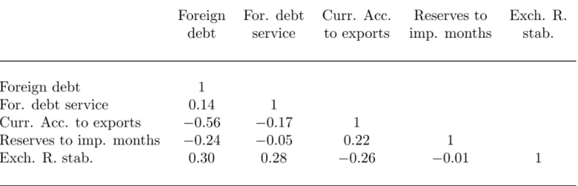
Table 9: Partial Correlations — Financial Risk Measures
Foreign For. debt Curr. Acc. Reserves to Exch. R. debt service to exports imp. months stab. Foreign debt 1
For. debt service 0:14 1
Curr. Acc. to exports 0:56 0:17 1
Reserves to imp. months 0:24 0:05 0:22 1
T a b le 1 0 : P a rt ia l C o rr el a ti o n s — P o li ti ca l R is k M ea su re s ICR G Go v t. So cio-e c. In v es tm . In ter n al E x te rnal P o liti cal M il itar y Religi ous La w and Ethn ic Demo c. B ureauc. ind ex stab. con dit. p ro… le con‡ ict con‡ ic t cor rup . in p oli tics tens ion s Order tens io n s acc o u n t. q u al it y ICR G inde x 1 Go v t. stab. 0 : 68 1 So cio-e c. cond it . 0 : 36 0 : 10 1 In v estm. pro… le 0 : 70 0 : 66 0 : 29 1 In te rn al con‡ ic t 0 : 72 0 : 51 0 : 25 0 : 48 1 External con‡ ict 0 : 53 0 : 35 0 : 03 0 : 32 0 : 46 1 P ol iti cal cor rup . 0 : 30 0 : 10 0 : 19 0 : 14 0 : 29 0 : 05 1 Milit ary in p oli tics 0 : 55 0 : 31 0 : 19 0 : 40 0 : 52 0 : 26 0 : 42 1 Religi ous ten sio n s 0 : 34 0 : 17 0 : 04 0 : 21 0 : 39 0 : 32 0 : 29 0 : 30 1 La w and Or d er 0 : 63 0 : 48 0 : 19 0 : 40 0 : 65 0 : 25 0 : 35 0 : 42 0 : 23 1 Eth nic ten sions 0 : 47 0 : 28 0 : 06 0 : 23 0 : 57 0 : 27 0 : 33 0 : 37 0 : 41 0 : 42 1 Demo c. acc o u n t. 0 : 33 0 : 18 0 : 05 0 : 25 0 : 21 0 : 28 0 : 35 0 : 44 0 : 14 0 : 16 0 : 20 1 Bureau c. quali ty 0 : 47 0 : 23 0 : 32 0 : 30 0 : 29 0 : 11 0 : 40 0 : 47 0 : 04 0 : 34 0 : 19 0 : 35 1
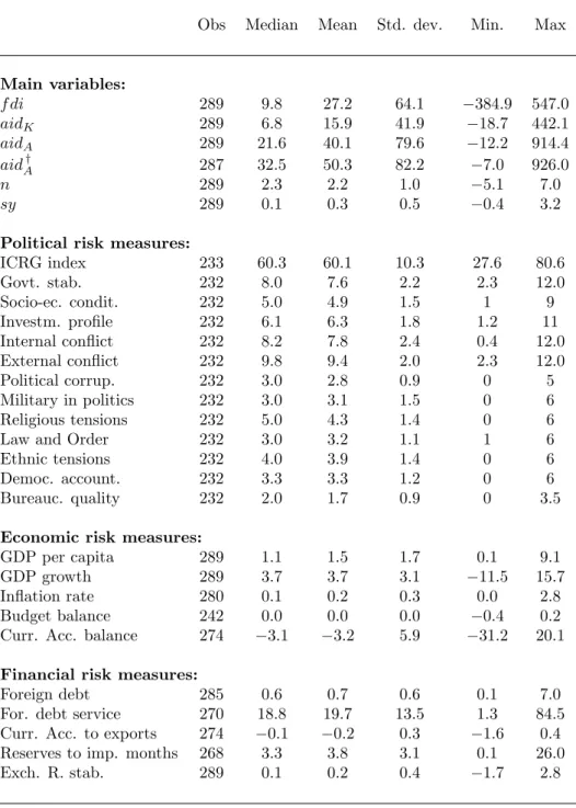
Table 11: Summary Statistics
Obs Median Mean Std. dev. Min. Max
Main variables: f di 289 9:8 27:2 64:1 384:9 547:0 aidK 289 6:8 15:9 41:9 18:7 442:1 aidA 289 21:6 40:1 79:6 12:2 914:4 aidAy 287 32:5 50:3 82:2 7:0 926:0 n 289 2:3 2:2 1:0 5:1 7:0 sy 289 0:1 0:3 0:5 0:4 3:2
Political risk measures:
ICRG index 233 60:3 60:1 10:3 27:6 80:6 Govt. stab. 232 8:0 7:6 2:2 2:3 12:0 Socio-ec. condit. 232 5:0 4:9 1:5 1 9 Investm. pro…le 232 6:1 6:3 1:8 1:2 11 Internal con‡ict 232 8:2 7:8 2:4 0:4 12:0 External con‡ict 232 9:8 9:4 2:0 2:3 12:0 Political corrup. 232 3:0 2:8 0:9 0 5 Military in politics 232 3:0 3:1 1:5 0 6 Religious tensions 232 5:0 4:3 1:4 0 6
Law and Order 232 3:0 3:2 1:1 1 6
Ethnic tensions 232 4:0 3:9 1:4 0 6
Democ. account. 232 3:3 3:3 1:2 0 6
Bureauc. quality 232 2:0 1:7 0:9 0 3:5
Economic risk measures:
GDP per capita 289 1:1 1:5 1:7 0:1 9:1
GDP growth 289 3:7 3:7 3:1 11:5 15:7
In‡ation rate 280 0:1 0:2 0:3 0:0 2:8
Budget balance 242 0:0 0:0 0:0 0:4 0:2
Curr. Acc. balance 274 3:1 3:2 5:9 31:2 20:1
Financial risk measures:
Foreign debt 285 0:6 0:7 0:6 0:1 7:0
For. debt service 270 18:8 19:7 13:5 1:3 84:5
Curr. Acc. to exports 274 0:1 0:2 0:3 1:6 0:4
Reserves to imp. months 268 3:3 3:8 3:1 0:1 26:0
T a b le 1 2 : S a m p le 7 5 -7 9 8 0 -8 4 8 5 -8 9 9 0 -9 4 9 5 -9 9 0 0 -0 1 7 5 -7 9 8 0 -8 4 8 5 -8 9 9 0 -9 4 9 5 -9 9 0 0 -0 1 A L B A lb a n ia M N G M o n g o li a A R G A r g e n t in a M O Z M o z a m b iq u e A R M A r m e n ia M R T M a u r it a n ia B D I B u r u n d i M U S M a u r it iu s B E N B e n in M W I M a la w i B F A B u r k in a F a s o M Y S M a la y s ia B G D B a n g la d e s h N A M N a m ib ia B G R B u lg a r ia N E R N ig e r B O L B o li v ia N G A N ig e r ia B R A B r a z il N IC N ic a r a g u a B W A B o t s w a n a N P L N e p a l C A F C e n t r a l A fr ic a n R e p . O M N O m a n C H L C h il e P A K P a k is t a n C H N C h in a P A N P a n a m a C IV C ô t e d ’I v o ir e P E R P e r u C M R C a m e r o o n P H L P h il ip p in e s C O G C o n g o , R e p . P R Y P a r a g u a y C O L C o lo m b ia R O M R o m a n ia C R I C o s t a R ic a R U S R u s s ia D O M D o m in ic a n R e p u b li c R W A R w a n d a D Z A A lg e r ia S A U S a u d i A r a b ia E C U E c u a d o r S D N S u d a n E G Y E g y p t S E N S e n e g a l E T H E t h io p ia S L V E l S a lv a d o r G H A G h a n a S Y R S y r ia G T M G u a t e m a la T C D C h a d H N D H o n d u r a s T G O T o g o H R V C r o a t ia T H A T h a il a n d H T I H a it i T J K T a ji k is t a n ID N In d o n e s ia T T O T r in id a d & T o b a g o IN D In d ia T U N T u n is ia IR N Ir a n T U R T u r k e y J A M J a m a ic a T Z A T a n z a n ia J O R J o r d a n U G A U g a n d a K A Z K a z a k s t a n U K R U k r a in e K E N K e n y a U R Y U r u g u a y K H M C a m b o d ia U Z B U z b e k is t a n L A O L a o s V E N V e n e z u e la L K A S r i L a n k a V N M V ie t N a m M A R M o r o c c o Y E M Y e m e n M E X M e x ic o Z A F S o u t h A fr ic a M L I M a li Z W E Z im b a b w e