Decision Support Systems

Data mining for credit card fraud: A comparative study

Siddhartha Bhattacharyya

⁎

_{, Sanjeev Jha}

_{, Kurian Tharakunnel}

_{, J. Christopher Westland}

Department of Information and Decision Sciences (MC 294), College of Business Administration, University of Illinois, Chicago, 601 South Morgan Street, Chicago, Illinois 60607-7124, USA b

Department of Decision Sciences, Whittemore School of Business and Economics, University of New Hampshire, McConnell Hall, Durham, New Hampshire 03824-3593, USA c_{Tabor School of Business, Millikin University, 1184 West Main Street, Decatur, IL 62522, USA}

d

Department of Information & Decision Sciences (MC 294), College of Business Administration, University of Illinois, Chicago, 601 S. Morgan Street, Chicago, IL 60607-7124, USA

a b s t r a c t

a r t i c l e i n f o

Available online 18 August 2010 Keywords:

Credit card fraud detection Data mining

Logistic regression

Credit card fraud is a serious and growing problem. While predictive models for credit card fraud detection are in active use in practice, reported studies on the use of data mining approaches for credit card fraud detection are relatively few, possibly due to the lack of available data for research. This paper evaluates two advanced data mining approaches, support vector machines and random forests, together with the well-known logistic regression, as part of an attempt to better detect (and thus control and prosecute) credit card fraud. The study is based on real-life data of transactions from an international credit card operation.

© 2010 Elsevier B.V. All rights reserved.

1. Introduction

Billions of dollars are lost annually due to credit card fraud[12,14]. The 10th annual online fraud report by CyberSource shows that although the percentage loss of revenues has been a steady 1.4% of online payments for the last three years (2006 to 2008), the actual amount has gone up due to growth in online sales[17]. The estimated loss due to online fraud is $4 billion for 2008, an increase of 11% on the 2007 loss of $3.6 billion [32]. With the growth in credit card transactions, as a share of the payment system, there has also been an increase in credit card fraud, and 70% of U.S. consumers are noted to be significantly concerned about identity fraud[35]. Additionally, credit card fraud has broader ramifications, as such fraud helps fund organized crime, international narcotics trafficking, and even terrorist

financing[20,35]. Over the years, along with the evolution of fraud detection methods, perpetrators of fraud have also been evolving their fraud practices to avoid detection[3]. Therefore, credit card fraud detection methods need constant innovation. In this study, we evaluate two advanced data mining approaches, support vector machines and random forests, together with the well-known logistic regression, as part of an attempt to better detect (and thus control and prosecute) credit card fraud. The study is based on real-life data of transactions from an international credit card operation.

Statistical fraud detection methods have been divided into two broad categories:supervised and unsupervised[3]. In supervised fraud detection methods, models are estimated based on the samples of

fraudulent and legitimate transactions, to classify new transactions as fraudulent or legitimate. In unsupervised fraud detection, outliers or unusual transactions are identi_fied as potential cases of fraudulent transactions. Both these fraud detection methods predict the probability of fraud in any given transaction.

Predictive models for credit card fraud detection are in active use in practice[21]. Considering the profusion of data mining techniques and applications in recent years, however, there have been relatively few reported studies of data mining for credit card fraud detection. Among these, most papers have examined neural networks [1,5,19,22], not surprising, given their popularity in the 1990s. A summary of these is given in[28], which reviews analytic techniques for general fraud detection, including credit card fraud. Other techniques reported for credit card fraud detection include case based reasoning[48]and more recently, hidden Markov models[45]. A recent paper[49]evaluates several techniques, including support vector machines and random forests for predicting credit card fraud. Their study focuses on the impact of aggregating transaction level data on fraud prediction performance. It examines aggregation over different time periods on two real-life datasets and finds that aggregation can be advantageous, with aggregation period length being an important factor. Aggregation was found to be especially effective with random forests. Random forests were noted to show better performance in relation to the other techniques, though logistic regression and support vector machines also performed well.

Support vector machines and random forests are sophisticated data mining techniques which have been noted in recent years to show superior performance across different applications [30,38,46,49]. The choice of these two techniques, together with logistic regression, for this study is based on their accessibility for practitioners, ease of use, and noted performance advantages in the literature. SVMs are statistical learning techniques, with strong ⁎ Corresponding author. Tel.: + 1 312 996 8794; fax: + 1 312 413 0385.

E-mail addresses:[email protected](S. Bhattacharyya),[email protected](S. Jha), [email protected](K. Tharakunnel),[email protected](J.C. Westland).

1

Tel.: + 1 603 862 0314; fax: + 1 603 862 3383. 2_{Tel.: + 1 312 996 2323; fax: + 1 312 413 0385.}

0167-9236/$–see front matter © 2010 Elsevier B.V. All rights reserved. doi:10.1016/j.dss.2010.08.008

Contents lists available atScienceDirect

Decision Support Systems

theoretical foundation and successful application in a range of problems [16]. They are closely related to neural networks, and through use of kernel functions, can be considered an alternate way to obtain neural network classifiers. Rather than minimizing empirical error on training data, SVMs seek to minimize an upper bound on the generalization error. As compared with techniques like neural networks which are prone to local minima, overfitting and noise, SVMs can obtain global solutions with good generalization error. They are more convenient in application, with model selection built into the optimization procedure, and have also been found to outperform neural networks in classification problems[34]. Appropriate param-eter selection is, however, important to obtain good results with SVM. Single decision tree models, though popular in data mining application for their simplicity and ease of use, can have instability and reliability issues. Ensemble methods provide a way to address such problems with individual classi_fiers and obtain good general-ization performance. Various ensemble techniques have been devel-oped, including mixture of experts, classifier combination, bagging, boosting, stacked generalization and stochastic gradient boosting (see [29]and[40]for a review for these). For decision trees, the random subspace method considers a subset of attributes at each node to obtain a set of trees. Random forests [6] combine the random subspace method with bagging to build an ensemble of decision trees. They are simple to use, with two easily set parameters, and with excellent reported performance noted as the ensemble method of choice for decision trees[18]. They are also computationally efficient and robust to noise. Various studies have found random forests to perform favorably in comparison with support vector machine and other current techniques[10,34].

The third technique included in this study is logistic regression. It is well-understood, easy to use, and remains one of the most commonly used for data-mining in practice. It thus provides a useful baseline for comparing performance of newer methods.

Supervised learning methods for fraud detection face two chal-lenges. The first is of unbalanced class sizes of legitimate and fraudulent transactions, with legitimate transactions far outnumber-ing fraudulent ones. For model development, some form of samploutnumber-ing among the two classes is typically used to obtain training data with reasonable class distributions. Various sampling approaches have been proposed in the literature, with random oversampling of minority class cases and random undersampling of majority class cases being the simplest and most common in use; others include directed sampling, sampling with generation of artificial examples of the minority class, and cluster-based sampling[13]. A recent experimental study of various sampling procedures used with different learning algorithms[25] found performance of sampling techniques to vary with learning algorithm used, and also with respect to performance measures. The paper also found that simpler techniques like random over and undersampling generally perform better, and noted very good overall performance of random undersampling. Random under-sampling is preferred to overunder-sampling, especially with large data. The extent of sampling for best performance needs to be experimentally determined. In this study, we vary the proportion of fraud to non-fraud cases in the training data using random undersampling, and examine its impact in relation to the three learning techniques and considering different performance measures.

The second problem in developing supervised models for fraud can arise from potentially undetected fraud transactions, leading to mislabeled cases in the data to be used for building the model. For the purpose of this study, fraudulent transactions are those specifi -cally identified by the institutional auditors as those that caused an unlawful transfer of funds from the bank sponsoring the credit cards. These transactions were observed to be fraudulent ex post. Our study is based on real-life data of transactions from an international credit card operation. The transaction data is aggregated to create various derived attributes.

The remainder of the paper is organized as follows.Section 2proves some background on credit card fraud. The next section describes the three data mining techniques employed in this study. InSection 4we discuss the dataset source, primary attributes, and creation of derived attributes using primary attributes. Subsequently, we discuss the experimental set up and performance measures used in our compar-ative study.Section 6presents our results and thefinal section contains a discussion onfindings and issues for further research.

2. Credit card fraud

Credit card fraud is essentially of two types: application and behavioral fraud[3]. Application fraud is where fraudsters obtaining new cards from issuing companies using false information or other people's information. Behavioral fraud can be of four types: mail theft, stolen/lost card, counterfeit card and_‘card holder not present_’fraud. Mail theft fraud occurs when fraudsters intercept credit cards in mail before they reach cardholders or pilfer personal information from bank and credit card statements[8]. Stolen/lost card fraud happens when fraudsters get hold of credit cards through theft of purse/wallet or gain access to lost cards. However, with the increase in usage of online transactions, there has been a significant rise in counterfeit card and‘card holder not present’fraud. In both of these two types of fraud, credit card details are obtained without the knowledge of card holders and then either counterfeit cards are made or the information is used to conduct‘card holder not present’transactions, i.e. through mail, phone, or the Internet. Card holders information is obtained through a variety of ways, such as employees stealing information through unauthorized_‘swipers_’,_‘phishing_’scams, or through intru-sion into company computer networks. In the case of‘card holder not present’ fraud, credit cards details are used remotely to conduct fraudulent transactions.

The evolution of credit card fraud over the years is chronicled in [50]. In the 1970s, stolen cards and forgery were the most prevalent type of credit card fraud, where physical cards were stolen and used. Later, mail-order/phone-order became common in the '80s and '90s. Online fraud has transferred more recently to the Internet, which provides the anonymity, reach, and speed to commit fraud across the world. It is no longer the case of a lone perpetrator taking advantage of technology, but of well-developed organized perpetrator communi-ties constantly evolving their techniques.

Boltan and Hand[4]note a dearth of published literature on credit card fraud detection, which makes exchange of ideas difficult and holds back potential innovation in fraud detection. On one hand academicians have dif_ficulty in getting credit card transactions datasets, thereby impeding research, while on the other hand, not much of the detection techniques get discussed in public lest fraudsters gain knowledge and evade detection. A good discussion on the issues and challenges in fraud detection research is provided in [4]and[42].

Credit card transaction databases usually have a mix of numerical and categorical attributes. Transaction amount is the typical numerical attribute, and categorical attributes are those like merchant code, merchant name, date of transaction etc. Some of these categorical variables can, depending on the dataset, have hundreds and thousands of categories. This mix of few numerical and large categorical attributes have spawned the use of a variety of statistical, machine learning, and data mining tools[4]. We faced the challenge of making intelligent use of numerical and categorical attributes in this study. Several new attributes were created by aggregating information in card holders' transactions over specific time periods. We discuss the creation of such derived attributes in more detail inSection 4of this paper.

Another issue, as noted by Provost[42], is that the value of fraud detection is a function of time. The quicker a fraud gets detected, the greater the avoidable loss. However, most fraud detection techniques need history of card holders' behavior for estimating models. Past

research suggests that fraudsters try to maximize spending within short periods before frauds get detected and cards are withdrawn[4]. Keeping this issue in mind we created _‘derived_’ attributes by aggregating transactions over different time periods to help capture change in spending behavior.

3. Data-mining techniques

As stated above, we investigated the performance of three techniques in predicting fraud: Logistic Regression (LR), Support Vector Machines (SVM), and Random Forest (RF). In the paragraphs below, we briefly describe the three techniques employed in this study.

3.1. Logistic regression

Qualitative response models are appropriate when dependent variable is categorical[36]. In this study, our dependent variablefraud

is binary, and logistic regression is a widely used technique in such problems [24]. Binary choice models have been used in studying fraud. For example,[26] used binary choice models in the case of insurance frauds to predict the likelihood of a claim being fraudulent. In case of insurance fraud, investigators use the estimated probabil-ities toflag individuals that are more likely to submit a fraudulent claim.

Prior work in related areas has estimated logit models of fraudulent claims in insurance, food stamp programs, and so forth [2,7,23,41]. It has been argued that identifying fraudulent claims is similar in nature to several other problems in real life including medical and epidemiological problems[11].

3.2. Support vector machines

Support vector machines (SVMs) are statistical learning techni-ques[47]that have been found to be very successful in a variety of classification tasks. Several unique features of these algorithms make them especially suitable for binary classification problems like fraud detection. SVMs are linear classifiers that work in a high-dimensional feature space that is a non-linear mapping of the input space of the problem at hand. An advantage of working in a high-dimensional feature space is that, in many problems the non-linear classification task in the original input space becomes a linear classification task in the dimensional feature space. SVMs work in the high-dimensional feature space without incorporating any additional computational complexity. The simplicity of a linear classifier and the capability to work in a feature-rich space make SVMs attractive for fraud detection tasks where highly unbalanced nature of the data (fraud and non-fraud cases) make extraction of meaningful features critical to the detection of fraudulent transactions is difficult to achieve. Applications of SVMs include bioinformatics, machine vision, text categorization, and time series analysis[16].

The strength of SVMs comes from two important properties they possess— kernel representation and margin optimization. In SVMs, mapping to a high-dimensional feature space and learning the classification task in that space without any additional computational complexity are achieved by the use of a kernel function. A kernel function[44]can represent the dot product of projections of two data points in a high-dimensional feature space. The high-dimensional space used depends on the selection of a speci_fic kernel function. The classification function used in SVMs can be written in terms of the dot products of the input data points. Thus, using a kernel function, the classification function can be expressed in terms of dot products of projections of input data points in a high-dimensional feature space. With kernel functions, no explicit mapping of data points to the higher-dimensional space happens while they give the SVMs the advantage of learning the classification task in that higher-dimen-sional space. The second property of SVMs is the way the best

classification function is arrived at. SVMs minimize the risk of overfitting the training data by determining the classification function (a hyper-plane) with maximal margin of separation between the two classes. This property provides SVMs very powerful generalization capability in classification.

In SVMs, the classi_fication function is a hyper-plane separating the different classes of data.

hw;xi+b= 0 ð1Þ

The notationhw;xirepresents the dot product of the coefficient vector w and the vector variable x.

The solution to a classification problem is then specified by the coefficient vector w. It can be shown thatwis a linear combination of data pointsxi⋅i= 1, 2,⋅⋅⋅,mi.e.,w=∑iaixi,ai≥0. The data pointsxi with non-zeroαiare called the support vectors.

A kernel functionk can be defined as k xð1;x2Þ=hΦð Þ;x1 Φð Þix2

whereΦ:X→His a mapping of points in the input space X into a higher-dimensional space H. As can be seen, the kernel function implicitly maps the input data points into a higher-dimensional space and return the dot product without actually performing the mapping or computing the dot product. There are several kernel functions suggested for SVMs. Some of the widely used kernel functions include, linear function, kðx1;x2Þ=hx1;x2i; Gaussian radial basis function

( R B F ) , kðx1;x2Þ=e−σtx1−x2t 2

a n d p o l y n o m i a l f u n c t i o n ,

kðx1;x2Þ=hx1;x2id. The selection of a specific kernel function for an

application depends on the nature of the classification task and the input data set. As can be inferred, the performance of SVMs is greatly depended on the specific kernel function used.

The classification function(1)has a dual representation as follows, whereyiare the classification labels of the input data points. ∑

i

aiγihxi;xi+b= 0

Using a kernel functionk, the dual classification function above in the high-dimensional space H can be written as

∑ i

aiγikðx1;xÞ+b= 0

As mentioned earlier, in SVMs, the best classification function is the hyper-plane that has the maximum margin separating the classes. The problem offinding the maximal margin hyper-plane can be formulat-ed as a quadratic programming problem. With the dual representation of the classification function above in the high-dimensional space H, the coefficients ai of the best classification function are found by solving the following (dual) quadratic programming problem.

maximize WðαÞ=∑m i= 1αi− 1 2∑ m i;j= 1αiαjγiγjkðxi;xjÞ subject to 0≤αi≤_mcði= 1;⋅⋅⋅;mÞ ∑m i= 1αiγi= 0

The parameter C in the above formulation is called thecost parameter

of the classification problem. The cost parameter represents the penalty value used in SVMs for misclassifying an input data point. A high value of C will result in a complex classification function with minimum misclassification of input data whereas a low value of C produces a classification function that is simpler. Thus, setting an appropriate value for C is critical to the performance of SVMs. The solution of the above quadratic programming problem is a computationally intensive task, which can be a limiting factor in using SVM with very large data.

However, iterative approaches like SMO[39]that can scale well to very large problems are used in SVM implementations.

3.3. Random forests

The popularity of decision tree models in data mining arises from their ease of use,flexibility in terms of handling various data attribute types, and interpretability. Single tree models, however, can be unstable and overly sensitive to specific training data. Ensemble methods seek to address this problem by developing a set of models and aggregating their predictions in determining the class label for a data point. A random forest[6]model is an ensemble of classification (or regression) trees. Ensembles perform well when individual members are dissimilar, and random forests obtain variation among individual trees using two sources for randomness:first, each tree is built on separate bootstrapped samples of the training data; secondly, only a randomly selected subset of data attributes is considered at each node in building the individual trees. Random forests thus combine the concepts of bagging, where individual models in an ensemble are developed through sampling with replacement from the training data, and the random subspace method, where each tree in an ensemble is built from a random subset of attributes.

Given a training data set of N cases described by B attributes, each tree in the ensemble is developed as follows:

- Obtain a bootstrap sample of N cases

- At each node, randomly select a subset of bbB attributes. Determine the best split at the node from this reduced set of b attributes

- Grow the full tree without pruning

Random forests are computationally ef_ficient since each tree is built independently of the others. With large number of trees in the ensemble, they are also noted to be robust to overfitting and noise in the data. The number of attributes, b, used at a node and total number of trees T in the ensemble are user-defined parameters. The error rate for a random forest has been noted to depend on the correlation between trees and the strength of each tree in the ensemble, with lower correlation and higher strength giving lower error. Lower values of b correspond to lower correlation, but also lead to lower strength of individual trees. An optimal value for b can be experimentally determined. Following[6]and as found to be a generally good setting for b in[27], we set b =_√B. Attribute selection at a node is based on the Gini index, though other selection measures may also be used. Predictions for new cases are obtained by aggregating the outputs from individual trees in the ensemble. For classification, majority voting can be used to determine the predicted class for a presented case.

Random forests have been popular in application in recent years. They are easy to use, with only two adjustable parameters, the number of trees (T) in the ensemble and the attribute subset size (b), with robust performance noted for typical parameter values[6]. They have been found to perform favorably in comparison with support vector machine and other current techniques[6,34]. Other studies comparing the performance of different learning algorithms over multiple datasets have found random forest to show good overall performance [9,10,27,31]. Random forests have been applied in recent years across varied domains from predicting customer churn[51], image classifi -cation, to various bio-medical problems. While many papers note their excellent classification performance in comparison with other tech-niques including SVM, a recent study[46]finds SVM to outperform random forests for gene expression micro-array data classification. The application of random forests to fraud detection is relatively new, with few reported studies. A recent paper[49]finds random forests to show superior performance in credit card fraud detection. Random forests have also been successfully applied to network intrusion detection [52], a problem that bears similarities to fraud detection.

4. Data

This section describes the real-life data on credit card transactions and how it is used in our study. It also describes the primary attributes in the data and the derived attributes created.

4.1. Datasets

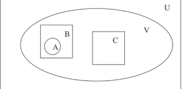
In this study we use the dataset of[37], which was obtained from an international credit card operation. The study in[37]used Artificial Neural Networks (ANN) tuned by Genetic Algorithms (GAs) to detect fraud. This dataset has 13 months, from January 2006 to January 2007, of about 50 million (49,858,600 transactions) credit card transactions on about one million (1,167,757 credit cards) credit cards from a single country. For the purpose of this study, we call this dataset of all transactions, dataset U (Fig. 1). A much smaller subset of this large dataset is dataset A, which has 2420 known fraudulent transactions with 506 credit cards.

One of the categorical attributes, transaction type, label transac-tions based on the kind of transaction, such as retail purchase, cash advance, transfer, etc. Suspecting fraud to be prevalent in only a few transaction types, we compared transaction types in the dataset A of observed fraudulent transactions with that in the full dataset U. We found that near 95% of observed fraudulent transactions (dataset A) were of retail purchase compared to less than 49% in dataset U (Table 1). Compared to dataset U, observed fraudulent transactions fell into only a few categories: retail types, non-directed payments, and check-item. Therefore, we partitioned the dataset U to include only the transaction types found in fraud dataset A. The reduced dataset U had 31,671,185 transactions and we call this reduced dataset as dataset V. To compare credit card fraud prediction using different techniques, we needed sets of transactions of both known fraudulent and undetected or observed legitimate transactions. Dataset A has cases of known fraudulent transactions, but we needed a comparable set of observed legitimate transactions. We decided to create a random sample of supposedly legitimate transactions from dataset V, excluding all transactions with the 506 fraudulent credit cards. Therefore, using dataset A and dataset V, wefirst created dataset B, which has all transactions in dataset V with these 506 credit cards. Dataset B has 37,280 transactions, of which the 2420 transactions in dataset A are the known fraudulent transactions. Next, we created dataset C, a random sample of observed legitimate transactions from dataset V minus the transactions in dataset B. The dataset C, observed legitimate transactions, has all transactions from 9645 randomly chosen credit cards. Dataset C has 340,589 credit card transactions.

The“Experimental Setup”section below details the creation of training and testing datasets using dataset A (observed fraudulent transactions) and dataset C (observed legitimate transactions).

4.2. Primary attributes

Primary attributes are attributes of credit card transactions available in the above datasets. We present these attributes inTable 2. Posting date attribute is the date of posting of transactions to the accounts. Account number attribute is the 16 digit credit card number of each transaction. Transaction type attribute categorizes transactions into types of transactions like cash advance, retail purchase, etc. Currency attribute provides the short code for the currency used to perform a transaction. Merchant code is the category code for the merchant for a given transaction. Foreign currency transaction, a binary attribute,flags a given transaction into whether a transaction is in foreign currency or not. Transaction date attribute is the date of a transaction. Merchant name, merchant city, and merchant country attributes describe the merchants of respective transactions. The acquirer reference code is a unique code for each transaction. E-commerceflag is a binary variable indicating if a transaction was an e-commerce transaction.

There are two quantitative attributes of credit card transactions in the dataset: foreign and local currency amount. Foreign currency amount is the amount of transaction made with a foreign merchant. Local currency amount is the amount of transaction in the local currency of the country where the card was issued.

We make a note here that although the dataset has transaction and posting dates of each transaction, there is no time stamp attribute available. In other words, in a given business day, we have no way to know the sequence of each transaction on a credit card. This is one of the limitations of the study and we discuss this again in sections below.

4.3. Derived attributes

As noted in[49], the high dimensionality and heterogeneity in credit card transactions make it impractical to use data on all transactions for a fraud detection system. They advocate employing a transaction aggregation strategy as a way to capture consumer spending behavior in the recent past. In this research, we employed a similar approach and created derived attributes from the primary attributes discussed in the previous section. The derived attributes provide aggregations on the transaction data. As mentioned in the above section, we have only two numerical attributes in our dataset: foreign currency amount and local currency amount. The other attributes were categorical. Hence, similar to[37], we created derived attributes for each transaction in the dataset to put each credit card transaction into the historical context of past shopping behavior. In essence, derived attributes provide information on card holders' buying behavior in the immediate past. For example, the practitioner literature suggests that consumer electronics category experience the highest fraud rate because it is easy to sell these products in electronic markets like eBay[32]. One of our derived attributes (Number merchant type over month) computes the number of transac-tions with a speci_fic merchant type over a month prior to a given transaction with a specific credit card. Now, for a given credit card

transaction, if there are a number of transactions with merchants in the consumer electronics category during the past month, then one may expect a higher likelihood of this transaction being fraudulent (based on practitioner literature), if it is to purchase consumer electronics. Similarly, we created other derived attributes for each transaction to aggregate immediate history of card holders' buying behavior. However, as mentioned above, since the data did not have specific time stamps for transactions, beyond the date of a transaction, the sequence of transactions with a credit card in a given day could not be determined. Hence, the derived attributes carried the same value for some of the attributes for transactions on a given day. For example, if a credit card has two transactions on a certain day, then without information on the sequence of these transactions, the derived attributes will have same value for both transactions since we do not know which of them took placefirst. Non-availability of time stamp data makes derived attributes less precise and this is a limitation of our study.Table 3lists the 16 derived attributes created and these are briefly described below:

Txn amount over month: average spending per transaction over a 30-day period on all transactions till this transaction. We computed the total amount spent with a credit card during the past 30 days prior to a transaction and divided it by the number of transactions to get the average amount spent.

Average over 3 months: average amount spent over the course of 1 week during the past 3 months. For this attribute, we computed the total amount spent with a credit card during the past 90 days prior to a transaction, and then divided it by 12 to get the average weekly spent over three months.

Dataset U: All transactions 49,858,600 transactions

Dataset A: Fraud Dataset 2,420 transactions

Dataset B: All transactions with Fraudulent Credit Cards 37,280 transactions Dataset V:All transactions with transaction types where fraud occurred 31,671,185 transactions Dataset C: Random sample of transactions from dataset V-B 340,589 transactions

U

V

B

A

C

Fig. 1.Dataset description.

Table 1

Percentage of credit card transactions by transaction types.

Transaction types Dataset U Dataset A

Retail purchase 48.65 94.67 Disputed transaction 15.58 0.00 Non-directed payment 14.15 0.50 Retail payment 8.85 0.00 Miscellaneous fees 4.11 0.00 Transaction code 3.91 0.00 Cash-Write-Off-Debt 1.30 0.00 Cash-Adv-Per-Fee 0.62 0.00 Check-Item 0.63 4.54 Retail-Adjust 0.01 0.00 Others 2.19 0.29 Total 100.00 100.00 Table 2

Primary attributes in datasets. Attribute name Description

Posting date Date when transaction was posted to the accounts Account number Credit Card number

Transaction type Transaction types, such as cash advance and retail purchase Currency Short code of the currency the transaction was originally

performed in

Merchant code Merchant Category Code

Foreign Txn Flagging whether this is a foreign currency transaction Transaction date Date when the transaction was actually performed Merchant name Name of merchant

Merchant city City of merchant Merchant country Country of merchant

Acquirer reference The reference code for the transactions E-commerce Flag if this was an Internet transaction

Foreign Txn Amt Foreign currency amount, the amount when transaction was made with a foreign merchant

Local Txn Amt The amount in the local currency of the country where the card is issued

Average daily over month: average spending per day over the past 30 days before this transaction. We calculated the total amount spent with a credit card during the past 30 days prior to a transaction and divided it by 30 to compute the average daily spent over a month prior to a transaction.

Amount merchant type over month: average spending per day on a merchant type over a 30-day period for each transaction. In this case, we_first computed the total amount spent with a credit card on a specific merchant type during the past 30 days prior to a transaction and then divided this sum by 30 to get the average money spent with a specific merchant type over a month prior to a transaction.

Number merchant type over month: total number of transactions with the same merchant over a period of 30 days before a given transaction. For this attribute, we computed the total number of transactions with a credit card with a specific merchant type during the past 30 days prior to a transaction.

Amount merchant type over3months: average weekly spending on a merchant type during the past 3 months before a given transaction. For this attribute, we computed the total amount spent with a credit card on a specific merchant type during the past 90 days prior to a transaction, and then divided it by 12 to get the average weekly amount spent over three months on that merchant type.

Amount same day: total amount spent with a credit card on the day of a given transaction. Here, for each transaction we computed the total amount spent in a day with that credit card.

Number same day: total number of transactions on the day of a given transaction. For this attribute, we computed the total number of transactions in a day with that credit card.

Amount same merchant: average amount per day spent over a 30 day period on all transactions up to this one on the same merchant as this transaction. In this case, we computed the total amount spent on the same merchant in the day of a given transaction with that credit card.

Number same merchant: total number of transactions with the same merchant during the last month. For this attribute, we computed the total number of transactions with the same merchant in the day of a given transaction with that credit card.

Amount currency type over month: average amount spent over a 30-day period on all transactions up to this transaction with the same currency. For this attribute, wefirst computed the total amount spent with a credit card on a specific currency type during past 30 days prior to a transaction and then divided this sum by 30 to get the average money spent with a speci_fic currency type over a month prior to a transaction.

Number currency type over month: total number of transactions with the same currency type during the past 30 days. For this attribute, we computed the total number of transactions with a credit card with a specific currency type during the past 30 days prior to a transaction.

Amount same country over month: average amount spent over a 30-day period on all transactions up to this transaction in the same country. For this attribute, wefirst computed the total amount spent with a credit card in a specific country during the past 30 days prior to a transaction and then divided this sum by 30 to get the average money spent in a specific country over a month prior to a transaction.

Number same country over month: total number of transactions in the same country during past 30 days before this transaction. In this case, we computed the total number of transactions with a credit card in a specific country during past 30 days prior to a transaction.

Amount merchant over3months: average amount spent over the course of 1 week during the past 3 months on the same merchant as this transaction. For this attribute, we computed the total amount spent with a credit card on a specific merchant during the past 90 days prior to a transaction, and then divided it by 12 to get the average weekly amount spent over three months on that merchant.

Number merchant over3months: total number of transactions with the same merchant during the past 3 months. For this attribute, we computed the total number of transactions with a credit card with a speci_fic merchant during the past 90 days prior to a transaction. 5. Experimental setup

The objective of this study is to examine the performance of two advanced data mining techniques, random forests and support vector machines, together with the well-known logistic regression, for credit card fraud identification. We also want to compare the effect of extent of data undersampling on the performance of these techniques. This section describes the data used for training and testing the models and performance measures used.

For our comparative evaluation, parameters for the techniques were set from what has been found generally useful in the literature and as determined from the preliminary tests on our data. No further

fine tuning of parameters was conducted. While fine tuning of

Table 3

Derived attributes used in models. Short Name Description Txn amount over

month

Average amount spent per transaction over a month on all transactions up to this transaction

Average over 3 months Average amount spent over the course of 1 week during past 3 months

Average daily over month

Average amount spent per day over the past 30 days Amount merchant type

over month

Average amount per day spent over a 30 day period on all transactions up to this one on the same merchant type as this transaction

Number merchant type over month

Total number of transactions with same merchant during past 30 days

Amount merchant type over 3 months

Average amount spent over the course of 1 week during the past 3 months on same merchant type as this transaction

Amount same day Total amount spent on the same day up to this transaction

Number same day Total number of transactions on the same day up to this transaction

Amount same merchant

Average amount per day spent over a 30 day period on all transactions up to this one on the same merchant as this transaction

Number same merchant

Total number of transactions with the same merchant during last month

Amount currency type over month

Average amount per day spent over a 30 day period on all transactions up to this one on the same currency type as this transaction

Number currency type over month

Total number of transactions in the same currency during the past 30 days

Amount same country over month

Average amount spent over a 30 day period on all transactions up to this one on the same country as this transaction

Number same country over month

Total number of transactions in the same country during the past 30 days before this transaction

Amount merchant over 3 months

Average amount spent over the course of 1 week during the past 3 months on same merchant as this transaction Number merchant over

3 months

Total number of transactions with the same merchant during the past 3 months

parameters to specific datasets can be beneficial, consideration of generally accepted settings is more typical in practice. The need for signi_ficant effort and time for parameter_fine tuning can often be a deterrent to practical use, and can also lead to issues of overfitting to specific data.

For SVM, we use Gaussian radial basis function as the kernel function which is a general-purpose kernel with good performance results. The cost parameter C and the kernel parameterσwere set to values 10 and 0.1 respectively. These values were selected after experimenting with different combinations of these values. For Random Forests, we set the number of attributes considered at a node, b =√B, where B is the total attributes in the data, and number of trees T = 200. Using T = 500 was found to result in slightly better performance, but at greater computationally cost.

5.1. Training and test data

Given the highly imbalanced data that is typical in such applications, data from the two classes are sampled at different rates to obtain training data with reasonable proportion of fraud to non-fraud cases. As noted earlier, random undersampling of the majority class has been found to be generally better than other sampling approaches[25]. We use random undersampling to obtain training datasets with varying proportions of fraud cases. We examine the performance of the different algorithms on four training datasets having 15%, 10%, 5% and 2% fraudulent transactions. These are labeled DF1, DF2, DF3, and DF4 in the results. Performance is observed on a separate Test dataset having 0.5% fraudulent transactions.

As described in the data section, dataset A has 2420 observed fraudulent transactions. We divided dataset A into two subsets of 1237 (51%) and 1183 (49%) transactions. We used thefirst set of 1237 fraudulent transactions in populating the four modeling datasets (DF1, DF2, DF3, and DF4) with fraudulent transactions and similarly the second set of 1183 transactions for populating the test dataset. We sampled legitimate transactions from dataset C to create varying fraud rates in the modeling and test datasets. In other words, we kept the same number of fraudulent transactions in the four modeling datasets, but varied the number of legitimate transactions from dataset C to create varying fraud rates. InTable 4, we show the composition of the modeling and test datasets. As shown inTable 4, the actual fraud rates in the four modeling datasets DF1, DF2, DF3, and DF4 were approximately 15%, 10%, 5%, and 2% respectively. Similarly, the actual fraud rates in the test dataset is 0.5%.

5.2. Performance measures

We use several measures of classification performance commonly noted in the literature. Overall accuracy is inadequate as a perfor-mance indicator where there is significant class imbalance in the data, since a default prediction of all cases into the majority class will show a high performance value. Sensitivity and specificity measure the accuracy on the positive (fraud) and negative (non-fraud) cases. A tradeoff between these true positives and true negatives is typically sought. The F-measure giving the harmonic mean of precision and recall, G-mean giving the geometric mean of fraud and non-fraud accuracies, and weighted-Accuracy provide summary performance indicators of such tradeoffs. The various performance measures are defined with respect to the confusion matrix below, where Positive corresponds to Fraud cases and Negative corresponds to non-fraud cases.

Predicted positive Predicted negative Actual positive True positives False negatives Actual negative False positives True negatives

Accuracy (TP + TN) / (TP + FP + TN + FN)

Sensitivity (or recall) TP / (TP + FN) gives the accuracy on the fraud cases.

Specificity TN / (FP + TN) gives the accuracy on the non-fraud cases. Precision TP / (TP + FP) gives the accuracy on cases predicted as

fraud.

F-measure 2 Precision Recall/(Precision + Recall). G-mean (Sensitivity Specificity)0.5_.

wtdAcc w Sensitivity + (1₋w) Speci_ficity; we use w = 0.7 to indicate higher weights for accuracy on the fraud cases. The above measures arising from the confusion matrix are based on a certain cutoff value for class-labeling, by default generally taken at 0.5. We also consider the AUC performance measure, which is often considered a better measure of overall performance [33]. AUC measures the area under the ROC curve, and is independent of specific classification cutoff values.

The traditional measures of classi_fication performance, however, may not adequately address performance requirements of specific applications. In fraud detection, cases predicted as potential fraud are taken up for investigation or some further action, which involves a cost. Accurate identification of fraud cases helps avoid costs arising from fraudulent activity, which are generally larger than the cost of investigating a potential fraudulent transaction. Such costs from undetected fraud will however be incurred for fraud cases that are not captured by the model. Fraud detection applications thus carry differential costs for false positives and false negatives. Performance measures like AUC, however, give equal consideration to false positives and false negatives and thus do not provide a practical performance measure for fraud detection[43]. Where cost informa-tion is available, these can be incorporated into a cost funcinforma-tion to help assess performance of different models[49].

We report on the multiple measures described above to help provide a broad perspective on performance, and since the impact of sampling can vary by technique and across performance measures [25]. Accuracy and AUC are among the most widely reported for classifier performance, though as noted above, not well suited for problems like fraud detection where significant class imbalance exists in the data. In evaluating credit card fraud detection, where non-fraud cases tend to dominate in the data, a high accuracy on the (minority class) fraud cases is typically sought. Accuracies on fraud and non-fraud cases are shown through sensitivity and specificity, and these, together with precision can indicate desired performance character-istics. The three summary measures indicate different tradeoffs amongst fraud and non-fraud accuracy. In implementation, a fraud detection model will be used to score transactions, with scores indicating a likelihood of fraud. Scored cases can be sorted in decreasing order, such that cases ranked towards the top have higher fraud likelihood. A well performing model here is one that ranks most fraud cases towards the top. With a predominance of non-fraud cases in the data, false positives are only to be expected. Model performance can be assessed by the prevalence of fraudulent cases among the cases ranked towards the top. The traditional measures described above do not directly address such performance concerns that are important in fraud management practice. We thus also consider the proportion of

Table 4

Training and testing datasets.

Training data Test data

Dataset DF1 Dataset DF2 Dataset DF3 Dataset DF4 Dataset T

Fraud 1237 1237 1237 1237 1183

Legitimate 6927 11,306 21,676 59,082 241,112 Total 8164 12,543 22,913 60,319 242,295 Fraud rate 15.2% 9.9% 5.4% 2.1% 0.5%

fraud cases among the top 1%, 5%, 10% and 30% of the total data set size. Results report the proportion of fraud cases among the top-K cases as ranked by the model scores, where K is the number of fraud cases in the data—a perfect model wouldfind all fraud cases among the top-K cases as ranked by model scores.

6. Results

This section presents results from our experiments comparing the performance of Logistic regression (LR), Random Forests (RF) and Support Vector Machines (SVM) model developed from training data carrying varying levels of fraud cases.

Wefirst present cross-validation results of the tree techniques on a training dataset having 10% fraud cases (DF2). Results are shown in Table 5for the traditional measures of classification performance. All differences are found to be signi_ficant (p_b0.01) except for Precision and F between LR and SVM, and for AUC between LR and RF. Wefind that RF shows overall better performance. LR does better than SVM on all measures other than specificity, precision and F. While these results help establish a basic and general comparison between the techniques, it is important to note that developed models in practice are to be applied to data with typically far lower fraud rates. We this next examine the performance of models developed using the different techniques on the separate test dataset.

The performance of LR, SVM and RF on traditional measures is shown inTable 6a,6b,6crespectively. For each technique, results are given for the four training datasets carrying different proportions of fraud. It is seen that Logistic Regression performs competitively with the more advanced techniques on certain measures, especially in comparison with SVM and where the class imbalance in training data is not large. It shows better performance than SVM on sensitivity except where the class imbalance in the training data becomes large (for DF4, with 2% fraud). The precision, F, G-mean and wtdAcc

measures show a similar comparison between LR and SVM. LR is also seen to exhibit consistent performance on AUC across the different training datasets. Random Forests show overall better performance than the other techniques on all performance measures.

The graphs in Fig. 2 highlight the comparison between the techniques across different training datasets, on various performance measures. Accuracy on the non-fraud cases, as given by specificity, is high, with RF showing an overall better performance. As may be expected, specificity increases with lower fraud rates in the training data, as more and more cases get classified into the majority class. As noted earlier, accuracy on the fraud cases is of greater importance for fraud detection applications, and sensitivity here is seen to decrease with lower fraud rates in the training data for all techniques; logistic regression, however, shows particularly low accuracy when the fraud rate in the training data is at the lowest level (DF4, 2% fraud). RF again shows the best performance, followed by LR and then SVM; for the training dataset with lowest fraud rate, however, SVM surpasses LR and performs comparably with RF. This pattern, with SVM matching the performance of RF when trained with the lowest proportion of fraud cases in the data, is also seen for the other measures. Precision increases with lower fraud rates in the training data; with fewer cases bring classi_fied as fraud, the accuracy of such fraud predictions improve. Here, again, RF shows highest performance; SVM and LR are similar, except for DF4, where SVM's performance approaches that of RF. On the F-measure, which incorporates a tradeoff between accuracy on fraud cases and precision in predicting fraud, RF shows markedly better performance; with the lowest fraud rate in the training data (DF4), SVM performs comparably with RF, with LR far lower. Performance on both the G-mean and wtdAcc measures, which take a combined consideration of accuracy on fraud and non-fraud cases, is similar to that for sensitivity.

The performance of LR is noteworthy on the AUC measure; while both RF and SVM show decreasing AUC with lower fraud rates in the

Table 5

Cross-validation performance of different techniques (training data M2 with 10% fraud rate).

acc Sensitivity Specificity Precision F AUC wtdAcc G-mean

LR 0.947 (0.004) 0.654 (0.053) 0.979 (0.004) 0.778 (0.027) 0.709 (0.029) 0.942 (0.014) 0.772 (0.039) 0.8 (0.032) SVM 0.938 (0.005) 0.524 (0.07) 0.984 (0.003) 0.782 (0.015) 0.624 (0.052) 0.908 (0.011) 0.678 (0.051) 0.716 (0.049) RF 0.962 (0.005) 0.727 (0.052) 0.987 (0.002) 0.86 (0.029) 0.787 (0.038) 0.953 (0.012) 0.818 (0.036) 0.847 (0.03) All differences significant (pb0.01) except for precision (LR, SVM), F(LR, SVM) and AUC (RF, SVM).

Table 6a

Performance of logistic regression across different fraud rates in training data.

LR acc Sensitivity Specificity Precision F WtdAcc G-Mean AUC

DF1: 15% fraud 0.966 0.740 0.967 0.100 0.177 0.808 0.846 0.925

DF2: 10% fraud 0.980 0.660 0.981 0.147 0.241 0.756 0.805 0.928

DF3: 5% fraud 0.987 0.527 0.989 0.188 0.277 0.666 0.722 0.928

DF4: 2% fraud 0.994 0.246 0.998 0.366 0.294 0.472 0.495 0.924

Table 6b

Performance of SVM across different fraud rates in training data.

SVM acc Sensitivity Specificity Precision F WtdAcc G-Mean AUC

DF1: 15% fraud 0.955 0.687 0.957 0.072 0.131 0.768 0.811 0.922

DF2: 10% fraud 0.980 0.593 0.982 0.139 0.226 0.710 0.763 0.922

DF3: 5% fraud 0.989 0.448 0.991 0.199 0.276 0.611 0.666 0.886

DF4: 2% fraud 0.996 0.430 0.998 0.567 0.489 0.601 0.655 0.818

Table 6c

Performance of random forest across different fraud rates in training data.

RF acc Sensitivity Specificity Precision F WtdAcc G-Mean AUC

DF1: 15% fraud 0.978 0.812 0.979 0.157 0.264 0.862 0.892 0.932

DF2: 10% fraud 0.987 0.747 0.988 0.233 0.355 0.819 0.859 0.934

DF3: 5% fraud 0.992 0.653 0.994 0.342 0.449 0.755 0.805 0.909

training data, LR is noticed to maintain a consistently good performance. AUC, unlike the other performance measures here, is independent of the classification threshold. Thus, where this threshold is irrelevant, LR models from different training data show similar AUC performance. Note that fraud cases across the different training datasets are the same, with only the non-fraud cases being sampled differentially in order to get different fraud rates in the training data. A consistently high value of AUC for LR across the training datasets indicates that the LR models maintain a similar ranking of cases, irrespective of the level of undersampling of non-fraud cases in the training data. This is also borne out by the non-fraud capture performance of LR given inTable 7a,7b,7c.

Table 7a,7breport performance with respect to the proportion of fraud cases captured at different data depths. Fig. 3 shows the proportion of fraud cases captured at 1%, 5%, 10% and 30% depths for

Fig. 2.Performance across different fraud rates in training data.

Table 7a

Proportion of fraud captured (logistic regression) in upperfile depths.

LR top-K 1% depth 5% depth 10% depth 30% depth M1: 15% fraud 0.298 0.456 0.806 0.886 0.964 M2: 10% fraud 0.313 0.473 0.804 0.880 0.975 M3: 5% fraud 0.305 0.464 0.798 0.883 0.977 M4: 2% fraud 0.308 0.461 0.798 0.876 0.967

models trained on the DF2 dataset (having 10% fraud rate). RF is seen to capture more of the fraud cases, with SVM and LR showing similar performance. With all techniques detecting greater number of fraud cases with increasing depth, the difference between RF and the other techniques gradually decreases. RF identifies around 90% of fraud cases in the test data at the 5% depth, while SVM and LR identify 80%. At 30% depth, most of the fraud cases are captured by all the techniques.

The graphs inFig. 4depict the proportion of fraud cases in the test data that are captured in the top-K, 1%, 5% and 30% depths. Recall that K here corresponds to the total fraud cases in the data; the top-K performance thus gives the proportion of fraud among the top-K cases as ranked by model scores. RF is clearly superior on this, capturing around 50% of the fraud cases in the top-K. The fraud capture performance in the top-K and top 1% depths shows an increasing trend for RF and SVM with smaller proportion of fraud in the training data. SVM, in particular, shows a marked increase in performance with smaller fraud rates in the training data. For LR, performance is consistent across the different fraud rates in training data.

At greater depths of 10% and 30%, where a large number of the fraud cases in the test data are captured, performance differences between the techniques is smaller. While RF still shows better performance at the 10% depth, this declines when the training data contains very low proportion of fraud cases (for DF4). Similar performance decline is also seen in SVM, for DF3 and DF4 training data. At the 30% depth, around 97% of the fraud cases are captured by all techniques; with lower fraud rates in the training data, however, the performance of RF and SVM decreases. LR, on the other hand, maintains consistent performance across the different training data, indicating, as noted above, that the LR models yield similar rankings among the cases, irrespective of the extent of undersampling of non-fraud cases in the training data.

7. Discussion

This paper examined the performance of two advanced data mining techniques, random forests and support vector machines, together with logistic regression, for credit card fraud detection. A real-life dataset on credit card transactions from the January 2006–

January 2007 period was used in our evaluation. Random forests and SVM are two approaches that have gained prominence in recent years with noted superior performance across a range of applications. Till date, their use for credit card fraud prediction has been limited. With the typically very low fraud cases in the data compared to legitimate transactions, some form of sampling is necessary to obtain a training dataset carrying an adequate proportion of fraud to non-fraud cases. We use data undersampling, a simple approach which has been noted to perform well [25], and examine the performance of the three

techniques with varying levels of data undersampling. The study provides a comparison of performance considering various traditional measures of classification performance and certain measures related to the implementation of such models in practice. For performance assessment, we use a test dataset with much lower fraud rate (0.5%) than in the training datasets with different levels of undersampling. This helps provide an indication of performance that may be expected when models are applied for fraud detection where the proportion of fraudulent transactions are typically low.

Encouragingly, all techniques showed adequate ability to model fraud in the considered data. Performance with different levels of undersampling was found to vary by technique and also on different performance measures. While sensitivity, G-mean and weighted-accuracy decreased with lower proportions of fraud in the training data, precision and specificity were found to show an opposite trend; on the F-measure and AUC, logistic regression maintained similar performance with varying proportions of fraud in the training data, while RF and SVM showed an decreasing trend on AUC and an increasing trend on F. Perhaps more informative from an application and practical standpoint is the fraud capture rate performance at different file depths. Here, random forests showed much higher performance at the upperfile depths. They thus capture more fraud cases, with fewer false positives, at the upper depths, an important consideration in real-life use of fraud detection models. Logistic regression maintained similar performance with different levels of undersampling, while SVM performance at the upper file depths tended to increase with lower proportion of fraud in the training data. Random forests demonstrated overall better performance across performance measures. Random forests, being computationally efficient and with only two adjustable parameter which can be set at commonly considered default values, are also attractive from a practical usage standpoint. Logistic regression has over the years been a standard technique in many real-life data mining applications. In our study, too, this relatively simple, well-understood and widely available technique displayed good performance, often surpassing that of the SVM models. As noted earlier, no deliberate attempts at optimizing the parameters of the techniques were made in this study. Parameter tuning can be important for SVM, and balanced sampling has been noted to be advantageous in using Random Forests on imbalanced data[15]. These carry the potential for better performance over that reported here and present useful issues for further investigation.

A factor contributing to the performance of logistic regression is possibly the carefully derived attributes used. Exploratory data analysis and variable selection is of course a time consuming step in the data mining process, and where such effort is in doubt, the performance of logistic regression may be uncertain. For ease of comparison, models from all techniques in our study were developed using the same derived attributes. Random forests and SVM carry natural variable selection ability and have been noted to perform well with high dimensional data. Their potential for improved perfor-mance when used on the wider set of available attributes is an interesting issue for further investigation.

Table 7b

Proportion of fraud captured (SVM) in upperfile depths.

SVM top-K 1% depth 5% depth 10% depth 30% depth M1: 15% fraud 0.244 0.363 0.697 0.855 0.970 M2: 10% fraud 0.269 0.437 0.802 0.857 0.970 M3: 5% fraud 0.326 0.439 0.620 0.771 0.930 M4: 2% fraud 0.474 0.606 0.786 0.795 0.810

Table 7c

Proportion of fraud captured (random forest) in upperfile depths.

RF top-K 1% depth 5% depth 10% depth 30% depth M1: 15% fraud 0.474 0.639 0.892 0.939 0.977 M2: 10% fraud 0.494 0.664 0.904 0.951 0.975 M3: 5% fraud 0.490 0.668 0.908 0.939 0.944 M4: 2% fraud 0.524 0.691 0.780 0.801 0.877

Future research can explore possibilities for creating ingenious derived attributes to help classify transactions more accurately. We created derived attributes based on past research, but future work can usefully undertake a broader study of attributes best suited for fraud modeling, including the issue of transaction aggregation[49]. Another interesting issue for investigation is how the fraudulent behavior of a card with multiple fraudulent transactions is different from a card with few fraudulent transactions. As mentioned above, a limitation in our data was the non-availability of exact time stamp data beyond the date of credit card transactions. Future study may focus on the difference in sequence of fraudulent and legitimate transactions before a credit card is withdrawn. Future research may also examine differences in fraudulent behavior among different types of fraud, say the difference in behavior between stolen and counterfeit cards.

Alternative means for dividing the data into training and test remains another issue for investigation. The random sampling of data into training and test as used in this study assumes that fraud patterns will remain essentially same over the anticipated time period of application of such patterns. Given the increasingly sophisticated mechanisms being applied by fraudsters and the potential for their varying such mechanisms over time to escape detection, such assumptions of stable patterns over time may not hold. Consideration of data drift issues can then become important. To better match how developed models may be used in real application, training and test data can be set up such that trained models are tested for their predictive ability in subsequent time periods. With availability of data covering a longer time period, it will be useful to examine the extent of concept drift and whether fraud patterns remain in effect over time.

References

[1] E. Aleskerov, B. Freisleben, B. Rao, CARDWATCH: a neural network based database mining system for credit card fraud detection, in computational intelligence for

financial engineering, Proceedings of the IEEE/IAFE, IEEE, Piscataway, NJ, 1998, pp. 220–226.

[2] M. Artis, M. Ayuso, M. Guillen, Detection of automobile insurance fraud with discrete choice models and misclassified claims, The Journal of Risk and Insurance 69 (3) (2002) 325–340.

[3] R.J. Bolton, D.J. Hand, Unsupervised profiling methods for fraud detection, Conference on Credit Scoring and Credit Control, Edinburgh, 2001.

[4] R.J. Bolton, D.J. Hand, Statistical fraud detection: a review, Statistical Science 17 (3) (2002) 235–249.

[5] R. Brause, T. Langsdorf, M. Hepp, Neural data mining for credit card fraud detection, Proceedings of the 11th IEEE International Conference on Tools with Artificial Intelligence, 1999, pp. 103–106.

[6] L. Breiman, Random forest, Machine Learning 45 (2001) 5–32.

[7] C.R. Bollinger, M.H. David, Modeling discrete choice with response error: food stamp participation, Journal of the American Statistical Association 92 (1997) 827–835.

[8] CapitalOne Identity theft guide for victims, retrieved January 10, 2009, from http: / / w w w . c a p i t a l o n e . c o m / f r a u d / I D T h e f t P a c k a g e V 0 1 2 1 7 2 0 0 4 W e . p d f ? linkid=WWW_Z_Z_Z_FRD_D1_01_T_FIDTP.

[9] R. Caruana, N. Karampatziakis, A. Yessenalina, An Empirical Evaluation of Supervised Learning in High Dimensions, in: Proceedings of the 25th international Conference on Machine Learning Helsinki, Finland, July, 2008.

[10] R. Caruana, A. Niculescu-Mizil, An Empirical Comparison of Supervised Learning Algorithms, in: Proceedings of the 23rd International Conference on Machine Learning, Pittsburgh, Pennsylvania, June, 2006.

[11] S.B. Caudill, M. Ayuso, M. Guillen, Fraud detection using a multinomial logit model with missing information, The Journal of Risk and Insurance 72 (4) (2005) 539–550.

[12] P.K. Chan, W. Fan, A.L. Prodromidis, S.J. Stolfo, Distributed Data Mining in Credit Card Fraud Detection, Data Mining, (November/December), 1999, pp. 67–74. [13] N.V. Chawla, N. Japkowicz, A. Kotcz, Editorial: special issue on learning from

imbalanced data sets, ACM SIGKDD Explorations Newsletter 6 (1) (2004). [14] R.C. Chen, T.S. Chen, C.C. Lin, A new binary support vector system for increasing

detection rate of credit card fraud, International Journal of Pattern Recognition 20 (2) (2006) 227–239.

[15] C. Chen, A. Liaw, L. Breiman, Using Random Forest to Learn Imbalanced Data, Technical Report 666, University of California at Berkeley, Statistics Department, 2004.

[16] N. Cristianini, J. Shawe-Taylor, An Introduction to Support Vector Machines and Other Kernel-based Learning Methods, Cambridge University Press, 2000. [17] CyberSource. Online fraud report: online payment, fraud trends, merchant practices,

and bench marks, retrieved January 8, 2009, from http://www.cybersource.com. [18] T.G. Dietterich, Ensemble learning, in: M.A. Arbib (Ed.), The Handbook of Brain

Theory and Neural Networks, Second edition, The MIT Press, Cambridge, MA, 2002. [19] J.R. Dorronsoro, F. Ginel, C. Sanchez, C. Santa Cruz, Neural fraud detection in credit

card operations, IEEE Transactions on Neural Networks 8 (1997) 827–834. [20] C. Everett, Credit Card Fraud Funds Terrorism, Computer Fraud and Security, May,

1, 2009.