MQ
I
TE WORKING PAPER SERIES
WP # 11-02
Does Stock Return Predictability Affect ESO Fair Value?
Does Stock Return Predictability Affect ESO Fair Value?
∗ Julio Carmona University of Alicante Angel Le´on University of Alicante Antoni Vaello-Sebasti`a† University of Illes Balears January 17, 2012Abstract
Executive Stock Options (ESOs) are modified American options that cannot be valued using standard methods. With a few exceptions, the literature has discussed the ESO fair value by assuming unpredictable stock returns which are not supported by the available empirical evidence. In this paper we obtain the fair value of American ESOs when stock returns are predictable and, specifically, driven by the trending Ornstein-Uhlenbeck process of Lo and Wang (1995). We solve the executive’s portfolio allocation problem for a simple buy-and-hold strategy when his wealth can be distributed between a risk-free asset and a market portfolio. This problem is jointly solved with the executive’s optimal exercise policy. We find that executives tend to wait longer the higher the predictability, independently of the composition of executive’s asset menu. We have also analyzed the implications under the FAS123R proposals for the ESO fair value and found that, even for low autocorrelations, there is a meaningful mispricing when unpredictable returns are erroneously assumed.
JEL Classification: G11, G13, G17, G35, M52
Keywords: Executive Stock Options, Risk Aversion, Undiversification, Predictability, FAS123R.
∗Angel Le´on and Antoni Vaello-Sebasti`a acknowledge the financial support from the Spanish Ministry for
Science and Innovation through the grants ECO2008-02599 and ECO2010-18567 respectively.
†Corresponding author: Antoni Vaello-Sebasti`a, Dpt. Economia de la Empresa, Universitat de les Illes
Balears, Palma de Mallorca, 07122, Illes Balears, Spain. Tel: +34 971 172024, fax: +34 971 172 389. E-mail: [email protected].
1
Introduction
Executive Stock Options (ESOs hereafter) are typically an important part of executive com-pensation packages. Hall and Murphy (2002) report that in 1999, 94% of S&P 500 companies granted ESOs to their top executives, and these grants accounted for 47% of total pay of S&P 500 CEOs. ESOs are American-style stock options modified for incentive reasons. Thus, ESOs cannot be sold or transferred, although partial hedge is possible by trading correlated assets. In addition, they can only be exercised after ending the vesting period. Consequently, standard methods for valuing American options are not directly applicable and a growing literature has been searching for a solution to the issue of ESO valuation.
A common assumption in this literature is that the stochastic process driving the dynamics of the underlying stock price can be represented as a geometric Brownian motion (GBM) process. Under this assumption, the stock returns turn out to be independent and identically distributed normal variates. However, there is by now a wide agreement in recognizing that this assumption does not fit well the empirical evidence concerning time series returns. As summarized, for instance, in Taylor (2005), there are three stylized facts characterizing the returns distribution at daily frequencies. First, the distribution of returns is not normal, it has typically fat tails with a high peak (leptokurtosis). Second, the autocorrelation of daily returns (predictability) is extremely low but statistically meaningful and third, there is positive dependence between squared returns. The impact on the ESO valuation of the last issue has been analyzed, among others, in Brown and Szimayer (2008), Le´on and Vaello-Sebasti`a (2009) and Yiang and Tian (2010). Nonetheless, to the best of our knowledge, modeling return autocorrelation in the stock price dynamics equation has been neglected in the literature of ESO valuation. There are two reasons for that. First, the constant drift term plays no role in the Black-Scholes (BS) formula according to the early result by Grundy (1991),1 who states that the BS formula still holds even though the underlying asset returns follow an Ornstein-Uhlenbeck (OU) process. Second, although the predictability of stock returns is now widely accepted by financial economists, there has been a long tradition in favor of the ”random walk” model for stock prices. Nonetheless, as we will show later, very low levels of autocorrelation generate significant biases in pricing ESOs.
1
Chapter 2 of Campbell et al. (1997) report autocorrelations for CRSP stock returns for both equally-weighted and value-weighted indexes. They find a statistically significant positive serial correlation at the first lag, which is robust across subsamples. The weekly and monthly return autocorrelations also exhibit a positive and statistically significant value at first lag over the entire sample and for all subsamples. Poterba and Summers (1988) also find negative autocorrelations for monthly CRSP data. Taylor (2005) surveys the evidence of predictability for several return series such as indexes, equities, futures and currencies for different time horizons and finds that these autocorrelations are very small but significant.2
For instance, more than 90% of the 600 autocorrelation estimates are between -0.05 and 0.05. These low but statistically significant autocorrelations imply that stock returns are predictable. Campbell and Yogo (2006) show more evidence of a predictable component in stock returns by building an efficient predictability test leading to valid inference regardless of the empirical evidence of high degree of persistence of the predictor variables (such as the dividend-price ratio, earnings-price ratio or measures of the interest rate).
This paper aims to analyze the effects of predictability in a restricted sense, namely, when return predictability comes only from their time series statistical properties. Therefore, we shall focus on univariate processes by following the same line of research as Lo and Wang (1995). They discuss the effect of predictability on the market value of European options by modeling initially a univariate trending Ornstein-Uhlenbeck (TOU) process, which is a continuous time AR(1) process. Under this setting, one can only model negative autocor-relations of returns. To model positive autocorautocor-relations, one has to resort to multivariate TOU processes already introduced by Lo and Wang (1995). Along these lines, in a constant volatility framework, they show that the autoregressive parameter has opposite effects on option prices, with negative (positive) autocorrelations increasing (decreasing) prices. This result is a peculiarity of the TOU process and does not hold in general.3
In any case, what Lo and Wang (1995) definitely show is that predictability of stock returns affects the prices of options written on those stocks. This is remarkable because in their set-up predictability is induced by the drift, which does not enter into the option pricing
2
More empirical references about the autocorrelation of returns can be seen in Taylor (2005).
3
For instance, Hafner and Herwartz (2001) show that there is no such asymmetry in discrete-time when the data generating probability measure follows an AR(1)-TGARCH(1,1) structure. Thus, the sign of the autoregressive parameter is irrelevant, all that matters is its size.
formula. The rationale is that, unlike the GBM process with a constant drift underlying the BS formula, the sample variance of discretely-sampled returns is not an appropriate estimator of the instantaneous variance when returns are predictable. Now, the estimation for the instantaneous variance is obtained as the sample variance adjusted by a factor that captures predictability depending on the first-order correlation coefficient of a discrete AR(1) process,4 which is the exact solution to the TOU process. Finally, observe that the closed-form option valuation they obtain corresponds, in our setting, to the firm’s cost of an European ESO for a risk-neutral executive.
Recent examples that can be found in the literature about the impact of stock returns predictability on the valuation of options are, among others, Liao and Chen (2006), Huang et al. (2009) and Paschke and Prokopczusk (2010). In the first paper, the stock return is modeled as a continuous-time MA(1)-type process. They show that the impact of autocor-related returns on European option prices is significant even when the MA(1) parameter is small. Contrary to the TOU process, the autocorrelated behavior of returns comes from the diffusion term. In the second paper, the authors propose an ARMA process for the stock return and model American options by using the local risk-neutralization principle of Duan (1995) and the Least squares Monte Carlo (LSM) approach by Longstaff and Schwartz (2001). They show that the AR effect is more significant than the MA effect in option pricing. Both papers refer to an earlier paper by Jokivuolle (1998), who values European options on au-tocorrelated indexes under a discrete-time framework. Finally, the third paper develops a continuous time factor model of commodity prices that allows for higher-order autoregressive and moving average components. In this set-up, they obtain closed-form pricing formulas for futures and options when the price dynamics are driven by a continuous autoregressive moving average (CARMA) process.5
Here, we are interested in the behavior of long-term American ESOs under predictability for returns driven by the TOU process and using the algorithm of Le´on and Vaello-Sebasti`a (2010), which is based on the LSM method, for the ESO valuation. As it is well known, we can distinguish among three possible ESO valuations depending on the restrictions faced by
4
See equations (11) and (12) below.
5
See Brockwell (2001) for a description of CARMA(p,q) models. Notice that the TOU process is, in fact, a CARMA(1,0) process.
the holder. The subjective value for the restricted executive, the objective value (the firm’s ESO cost) for the issuing firm, which is unrestricted but obliged to follow the executive’s exercise policy, and the market (risk-neutral) value for an unrestricted holder. This value is just the ESO objective value for a risk-neutral executive. Although we are only interested on the implications of predictability in stocks returns for the objective valuation of ESOs, we will also analyze the subjective valuation since this will allow us to infer the executive’s exercise policy required to obtain the objective value.
The rest of the paper is organized as follows. Section 2 presents the setting for ESO valuation. We distinguish between the case in which the ESO cost is driven by only the stock price, or the one state-variable (S1) model, which corresponds to the framework put forward initially by Hall and Murphy (2002), and the case in which the ESO cost is also affected by the availability of a market portfolio, or the two state-variable (S2) model, introduced by Cai and Vijh (2005). Section 3 presents our results concerning the S1 model. In this section we perform an extensive sensitivity analysis examining the size and sign of the bias that is incurred when the objective ESO value is obtained by assuming a GBM process for the stock price. In Section 4, we include a market portfolio as an additional investment for the executive’s wealth and show the differences in the results because of its introduction. In Section 5, we apply our framework to evaluate the bias induced by the computation of the firm’s ESO cost using the FAS123R method. Section 6 concludes. We have also included three appendices corresponding to Section 2. In Appendix A, we show the exact solution of the TOU process and its properties. Appendix B, we provide a detailed description of the algorithm mentioned above for valuing both, objective and subjective ESOs. Finally, Appendix C summarizes the optimization and numerical details to obtain the ESO subjective valuation.
2
Model description
To analyze how predictability affects the firm’s ESO cost, we need to obtain previously the executive’s exercise policy. This exercise policy is characterized, as usual, by a threshold price and it comes from solving the ESO subjective valuation problem. Then, by using the risk-neutral measure and the threshold price, the ESO objective value follows. See, for instance,
Kulatilaka and Marcus (1994), Hall and Murphy (2002) or Ingersoll (2006).
2.1 The set-up
We assume an environment in which the executive has an initial wealth, 𝑊0, of which a
proportion𝛼 is held in restricted stocks of the company that cannot be sold until the ESO maturity. The larger𝛼, the more related is the executive’s wealth to the firm’s market value and so, the higher the idiosyncratic risk supported. The remainder of the initial wealth, (1−𝛼)𝑊0, is distributed between the market portfolio and the risk-free asset in proportions
𝜂 and 1−𝜂 respectively. This composition is decided at time 0, the grant date, and held unchanged until the end of the planning period, given by the ESO maturity, at time 𝑇. In other words, we assume the executive follows a buy-and-hold strategy for both market asset and risk-free holdings. This is in line with Barberis (2000), who also incorporates the effects of predictability. Of course, a more realistic situation would allow𝜂 to vary across the investment horizon period. But, since we also need to find at the same time the executive’s exercise policy, such a strategy becomes hard to compute and the implementation of both situations are beyond the scope of our study.
Next, the executive is granted with an amount of𝑁 at-the-money ESOs with an exercise price of𝐾. Thus, the executive wealth at maturity is conditioned on the ESO exercise date. Let us denote by 𝑊𝑇∣𝑡 the executive’s wealth at maturity conditional on the ESO exercise at time 𝑡≤𝑇. Then, if the ESOs are not exercised until maturity, the executive’s terminal wealth is 𝑊𝑇∣𝑇 =𝛼𝑊0𝑒𝑞 𝑇¯ 𝑆𝑇 𝑆0 +( 1−𝛼) 𝑊0 ( 𝜂𝑀𝑇 𝑀0 +( 1−𝜂) 𝑒𝑟𝑓𝑇 ) +𝑁( 𝑆𝑇 −𝐾 )+ , (1)
where𝑆𝑇 and 𝑀𝑇 denote the firm’s stock and market portfolio prices at date𝑇. The yearly stock dividend yield, denoted as ¯𝑞, is assumed to be reinvested in restricted stocks.6 The
main point here is that the executive does not receive any payment from restricted stocks until𝑇. Finally, 𝑟𝑓 denotes the yearly risk-free rate.
Given our assumed buy-and-hold strategy for the executive’s portfolio, if the ESOs are
6
For simplicity, this model assumes that the investment in the market portfolio is done through an index fund, which does not pay dividends since it reinvests all dividend proceeds.
exercised at time 𝑡 < 𝑇, he will invest the ESO proceeds according to the same initial combination of market portfolio and risk-free asset. Thus,
𝑊𝑇∣𝑡 = 𝛼𝑊0𝑒𝑞 𝑇¯ 𝑆𝑇 𝑆0 +( 1−𝛼) 𝑊0 ( 𝜂𝑀𝑇 𝑀0 +( 1−𝜂) 𝑒𝑟𝑓𝑇 ) + + 𝑁( 𝑆𝑡−𝐾 )+ ( 𝜂𝑀𝑇 𝑀𝑡 +( 1−𝜂) 𝑒𝑟𝑓(𝑇−𝑡) ) . (2)
Notice that, despite the ESO exercise, the executive must maintain his restricted stocks until 𝑇. We shall assume that 𝑀𝑡 follows a GBM process driven by
𝑑𝑀𝑡=𝜇𝑀𝑀𝑡𝑑𝑡+𝜎𝑀𝑀𝑡𝑑𝑍𝑀,𝑡 , (3)
while𝑝𝑡≡ln𝑆𝑡 follows a trending Ornstein-Uhlenbeck (TOU) process:
𝑑𝑝𝑡= ( 𝜃−𝜅( 𝑝𝑡−𝜃𝑡 )) 𝑑𝑡+𝜎𝑑𝑍𝑆,𝑡 , (4)
where𝜅≥0 and 𝑑𝑍𝑆,𝑡𝑑𝑍𝑀,𝑡=𝜌𝑑𝑡. Notice that the TOU process includes the GBM process as a particular case when𝜅= 0. We can rewrite equation (4) as
𝑑(
𝑝𝑡−𝜃𝑡
)
=−𝜅(𝑝𝑡−𝜃𝑡)𝑑𝑡+𝜎𝑑𝑍𝑆,𝑡 . (5)
Note that, when𝑝𝑡 deviates from its trend𝜃𝑡, it is pulled back at a rate𝜅, the speed of mean reversion, proportional to its deviation.7
The executive is endowed with a standard power utility function defined over his terminal wealth: 𝑈( 𝑊𝑇 ) = ⎧ ⎨ ⎩ 𝑊𝑇1−𝛾 1−𝛾 if𝛾 ∕= 1 ln( 𝑊𝑇 ) if𝛾 = 1, (6)
where𝛾 >0 is the coefficient of relative risk-aversion.
The executive maximizes the expected utility of his terminal wealth allocating his outside wealth between the market portfolio and the risk-free asset to their optimal sizes, denoted as 𝜂∗ and 1−𝜂∗ respectively, and selecting his optimal ESO exercise date, 𝑡∗. Therefore, the
7
executive’s maximum expected utility is given by 𝑈∗ ≡max 𝜂,𝑡 E0 [ 𝑈( 𝑊𝑇∣𝑡 )] . (7)
In short, we assume an asset allocation framework for a buy-and-hold investor (the executive) regarding both risk-free and market asset holdings.
2.2 Model implementation
The methodology used to solve the program described by equation (7) is a modified version of the LSM algorithm of Longstaff and Schwartz (2001) for pricing path dependent derivatives. It consists on two stages. In the first stage, equation (7) is solved for a grid of values of𝜂. This yields the executive’s exercise policy, defined by a unique threshold price, for each𝜂 in the grid. Observe that we also obtain the corresponding expected exercise date,𝜏, for each 𝜂 in the grid. Appendix B provides a detailed description of how these values are obtained. Then, in a second stage, we select the corresponding values for both the market portfolio share and the threshold price denoted, respectively, as 𝜂∗ and 𝑆∗, yielding the maximum
executive’s expected utility. Finally, after finding 𝑆∗, we can solve for the ESO objective
value,𝑉𝑂𝐵𝐽, using the risk-neutral measure.
We next obtain the executive’s subjective valuation using the certainty-equivalence prin-ciple already introduced by Lambert et al. (1991). It identifies the subjective ESO value with the amount of cash that, delivered at the grant date and invested until ESO maturity, reports the same expected utility to the executive than holding the ESO. This is obtained as follows. Suppose that, at the grant date, a non-restricted amount of cashCEis delivered in place of each ESO. Then, the total executive’s wealth at maturity is
𝑊𝑇𝐶𝐸 =𝛼𝑊0𝑒𝑞 𝑇¯ 𝑆𝑇 𝑆0 +[( 1−𝛼) 𝑊0+𝑁 ⋅CE ] ( 𝜂𝑀𝑇 𝑀0 +( 1−𝜂) 𝑒𝑟𝑓𝑇 ) . (8)
Thus, to calculate the subjective value we only need to find the amount CE that provides the same expected utility than holding an amount𝑁 of ESOs. Therefore, as in Tian (2004)
,CEsolves the following equation: max 𝜂 E0 [ 𝑈( 𝑊𝑇𝐶𝐸 )] =𝑈∗. (9)
where𝑈∗ is given in equation (7). Notice that, for this maximization program, the optimal
market portfolio share in executive’s wealth will be, in general, different from that obtained when the executives chooses optimally the ESOs exercise date (𝑡∗) and the proportion of unrestricted wealth to be allocated into the market portfolio (𝜂∗). 8
Although the paper is not concerned with the properties of the executive’s subjective valuation under predictability of stock returns, we can illustrate some of them with the help of Figure 1. In this figure we have plotted the ratio of the executive’s subjective valuation when returns are predictable,CE𝑇 𝑂𝑈, with respect to the case of no predictability driven by a GBM process,CE𝐺𝐵𝑀. In both cases, the executive’s unrestricted wealth can be allocated only in the risk-free asset. Clearly, as one should expect, this ratio increases with the predictability of returns. Furthermore, the ratio is higher the higher the degree of risk-aversion or the higher the weight of restricted stocks on executive’s wealth.
2.3 Discrete-time return for the TOU process
To implement our model we use the exact time solution of equation (5). The discrete-time return at discrete-time𝑡for a time period of length ℎ is defined as
𝑟𝑡,ℎ ≡ln ( 𝑆𝑡 ) −ln( 𝑆𝑡−ℎ ) . (10)
Then, the mean of𝑟𝑡,ℎ equals𝜃ℎ. Whenℎ is measured as a fraction of a year,𝜃measures the annual mean of log-return. Similarly, the variance, 𝜎𝑟2, and the autocorrelation at lag one, 𝜌𝑟(1), of the discrete-time returns are related to the speed of mean reversion according to the following expressions:
8
We are indebted to an anonymous referee for pointing this to us. Further details about the optimization are explained in Appendix C.
Figure 1: Behavior of the subjective ESO value as a function of predictability, 𝜅. 0 0.05 0.1 0.25 0.5 0.75 1 1.5 2 2.5 3 3.5 4 4.5 5 κ CE TOU / CE GBM No vesting 0 0.05 0.1 0.25 0.5 0.75 1 1.5 2 2.5 3 3.5 4 4.5 5 κ Vesting = 3 years γ = 2, α = 1/2 γ = 2; α = 2/3 γ = 4; α = 1/2 γ = 4; α = 2/3
This figure plots the ratio between the subjective value when the stock price is driven by a TOU process, CE𝑇 𝑂𝑈, and the corresponding one when the stock price is driven by a GBM process, CE𝑇 𝑂𝑈, as a function
of the speed of adjustment parameter,𝜅. Other parameters used for the TOU process are𝜃 = 0.10 and
𝜎 = 0.30. The remaining parameters describing the executive environment are those detailed at the beginning of Section 3. 𝜎2𝑟 = 𝜎 2 𝜅 ( 1−𝑒−𝜅ℎ) , (11) 𝜌𝑟(1) = − 1 2 ( 1−𝑒−𝜅ℎ), (12)
where to simplify notation, the dependence of the former definitions onℎ has been omitted. Now, as equations (11) and (12) make clear, when𝜅increases,𝜎2𝑟decreases but𝜌𝑟(1) increases in absolute value. Finally, observe that the value𝜅= 0 nests the case of a GBM process for the stock price, for which autocorrelations of log-returns are zero at all lags.
3
The one state-variable framework
In this section we focus on𝑉𝑂𝐵𝐽, that is obtained by using the risk-neutral measure to value an American call option for which the threshold price is defined by the executive’s exercise policy. We proceed in two stages. At first, we assume executives will have no availability to a market portfolio to allocate their unrestricted wealth, so that, the parameter𝜂is restricted
to be equal to zero. We have denoted this framework as the𝑆1 model, since the stock price is the only state-variable to obtain 𝑉𝑂𝐵𝐽. We consider this simplified version of the model because the computational cost is much lower (we do not have to find𝜂∗) and the main results are also valid in the more general case. Nonetheless, in Section 4 we extend our framework to include the availability of the market portfolio, in addition to the risk-free asset and the firm’s stock, giving place to the S2 model to get𝑉𝑂𝐵𝐽.
Following the benchmark case by Hall and Murphy (2002), we consider a representative executive that owns five million dollars in initial wealth and is granted with 150,000 stock options issued at-the-money with𝐾 = $1. We maintain as the true data generating process (DGP) for the stock price the TOU process, as described in equation (5). We explore how 𝑉𝑂𝐵𝐽 changes as a result of changes in each of the three parameters characterizing the above process. Our benchmark (yearly) values for these parameters are: 𝜅 = 0.50 for the speed of adjustment, 𝜃 = 0.10 for the long-run drift coefficient, and 𝜎 = 0.30 for the diffusion coefficient. Other parameter values are𝑟𝑓 = 0.06 and ¯𝑞= 0.
According to equation (12) and for our benchmark value of 𝜅 = 0.50, 𝜌𝑟(1) is equal to −0.020 in monthly terms (ℎ= 1/12),−0.005 in weekly terms (ℎ= 1/52) and−0.001 in daily terms (ℎ= 1/360). This low value of𝜌𝑟(1) can be found in the empirical evidence, see Table 4.8 in Taylor (2005). Although it may seem low, it will help us to highlight, in a later section, the mispricing that can be incurred in the computation of𝑉𝑂𝐵𝐽 if a standard GBM process, that exhibits independent returns, is postulated erroneously as the true DGP for the stock price.
Now, we are mainly concerned with the consequences of the evidence of stock return predictability on 𝑉𝑂𝐵𝐽. A greater predictability is, in the present setting, a higher size of 𝜌𝑟(1). Since the autocorrelations for stock returns found in empirical studies are generally so low, the GBM process might be a good approximation for the DGP of stock prices. However, under the true DGP these small autocorrelations come from a mean reversion process such as the TOU process in equation (5).
All this suggests that we are interested in analyzing how changes in 𝜌𝑟(1), and hence changes in 𝜅, affect 𝑉𝑂𝐵𝐽. Therefore, to control for the change in the volatility of the discrete-time returns, 𝜎𝑟, resulting from a change in 𝜅, we have also adjusted the diffusion
coefficient, 𝜎, in order to keep 𝜎𝑟 unchanged. To be sure that nothing is lost by imposing this restriction, we have also examined the case in which𝜎 is not adjusted, so that changes in 𝜅 also modify 𝜎𝑟. It has turned out that the differences between both cases, in terms of objective valuation, average exercise dates and other features of interest, have not been significant. Thus, we focus on the case in which𝜎 is adjusted so as to keep𝜎𝑟 constant.
Considering the above adjustment, a higher𝜅implies only an increase in the size of𝜌𝑟(1). The range of values for 𝜅, between 0 and 1, implies a range of first-order autocorrelations between 0 and 0.04 in monthly terms, which are representative of the values found in the empirical literature cited previously. For the diffusion coefficient, 𝜎, the values range from 𝜎= 0.25 to𝜎 = 0.45, and for the long-run drift coefficient,𝜃, the values range from𝜃= 0.065 to𝜃= 0.15.
3.1 Discussion of results
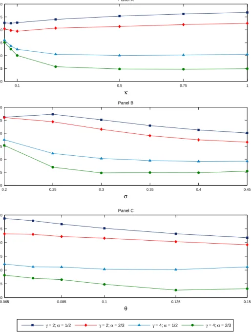
We study now the impact of changes in𝜅,𝜎 and𝜃in the ESO valuation. Figure 2 summarizes our main findings concerning the behavior of𝑉𝑂𝐵𝐽 as a function of these parameters. In all simulations we have considered the case of a 10-year ESO with a vesting period of 3 years, which is common in both practice and literature. The no vesting case is qualitatively similar and it is omitted to save space.
Several features can be observed in this figure. First, as 𝜅 increases, which means a higher predictability, 𝑉𝑂𝐵𝐽 seems to converge independently of the size for 𝛾 and 𝛼 (panel A). Second, an increase in either𝜎 (panel B) or𝜃(panel C) supposes a higher value of𝑉𝑂𝐵𝐽. Thus, as one would expect, the objective valuation increases with the diffusion coefficient,𝜎, and this is independent of the values considered for𝛾 and 𝛼. Clearly, a higher 𝜎 implies a higher𝜎𝑟, which leads to higher stock prices in relatively shorter periods of time.
However, the positive relationship between 𝜃 and 𝑉𝑂𝐵𝐽 may be somewhat surprising. According to the Black-Scholes model, the expected returns are irrelevant for option pricing. Nonetheless, in the present framework𝜃 affects the executive’s exercise behavior, and hence the ESO objective valuation. With greater expected returns, a higher 𝜃, it will be more profitable for the executive to hold the ESOs for a longer period. Then, higher expected returns could mitigate the executive’s suboptimal early exercise.
Figure 2: Behavior of the objective ESO value in the S1 framework. 0.1 0.5 0.75 1 −20 −15 −10 −5 0 5 10 Panel A κ Bias 1 0.2 0.25 0.3 0.35 0.4 0.45 −20 −15 −10 −5 0 5 10 Panel B σ Bias 1 0.065 0.085 0.1 0.125 0.15 −20 −15 −10 −5 0 5 10 Panel C θ Bias 1 γ = 2; α = 1/2 γ = 2; α = 2/3 γ = 4; α = 1/2 γ = 4; α = 2/3
We show the behavior of the objective ESO’s value for a 10-year ESO with a vesting period of 3 years,
𝑉𝑂𝐵𝐽, is represented as a function of the speed of adjustment,𝜅, in panel A; the diffusion coefficient,𝜎, in
panel B and the long-run drift,𝜃, in panel C. In each panel we have considered two values for the degree of relative risk-aversion,𝛾={2,4}, and for the degree of undiversification,𝛼={1/2,2/3}. The other values for the parameters of the TOU process in equation (5) are: 𝜃= 0.10 and𝜎= 0.30 for panel A;𝜅= 0.50 and𝜃= 0.10 for panel B, and𝜅= 0.50 and𝜎= 0.30 for panel C. In all cases, we have set𝑟𝑓 = 0.06 and
¯
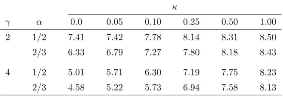
Table 1: Average exercise dates (in years) and predictability. 𝜅 𝛾 𝛼 0.0 0.05 0.10 0.25 0.50 1.00 2 1/2 7.41 7.42 7.78 8.14 8.31 8.50 2/3 6.33 6.79 7.27 7.80 8.18 8.43 4 1/2 5.01 5.71 6.30 7.19 7.75 8.23 2/3 4.58 5.22 5.73 6.94 7.58 8.13
This table collects the results concerning how the average exercise dates, 𝜏∗, of
our 10-year ESO are affected by different values of mean reversion,𝜅, which drives the autocorrelation of the TOU process in equation (5), respecting different levels of𝛾 and𝛼. The column for𝜅= 0 presents the values of𝜏∗for the corresponding
equivalent GBM process as described in Appendix A. For all cases, the risk-free rate, the dividend yield, the ESO maturity and the length of the vesting period have been set to their benchmark values, namely, 𝑟𝑓 = 0.06, ¯𝑞= 0,𝑇 = 10 and
𝜈= 3.
By definition,𝑉𝑂𝐵𝐽 depends on the executive’s exercise policy. This exercise policy can be described in terms of either the threshold price,𝑆∗, or the expected exercise time,𝜏∗. We
next examine the former results in connection with the obtained values for𝜏∗. The relevant
results are presented in Tables 1 and 2.
As Table 1 shows, higher values of 𝜅 imply higher values of 𝜏∗ for all considered com-binations of 𝛾 and 𝛼. Of course, either a higher 𝛾 or 𝛼 makes the executive to exercise comparatively earlier but, as𝜅 increases, these differences become smaller. Furthermore, the expected exercise time is comparatively lower for the equivalent GBM process,9 for which 𝜅= 0, in all cases.
To understand the role of predictability in the observed behavior for 𝑉𝑂𝐵𝐽 and 𝜏∗, we
examine Figure 3 in which we have plotted several simulated paths for the firm’s stock price under alternative values of𝜅.10 We have also plotted the long-run trend of the process by a
discontinuous line. As it can be observed, as𝜅increases from 0.05 to 1.00 (i.e. 𝜌𝑟(1) changes
9
This GBM process for stock prices has been constructed in such a way that the mean and variance of the discrete-time returns are the same than the corresponding ones for the true TOU process. More details are given in Appendix A.
10
To isolate the effects of predictability, the monthly volatility for discrete returns remains constant to 0.0866 in all cases and the four simulated paths in each panel are generated using the same random numbers. Then, the observed differences only depend on𝜅. The other relevant parameters have been set to𝜃 = 0.10 and𝜎= 0.30 in all simulations.
from −0.002 to −0.04), the simulated paths tend to revert faster to that long-run trend, avoiding the paths become very deep in-the-money. Then, as long as the time to maturity is kept fixed, the average values achieved by the TOU process are comparatively lower the higher𝜅. Hence, the executive tends to postpone the ESO exercise increasing, accordingly, the value of𝜏∗.
Therefore when prices are weakly mean reverting, so that they resemble closely a GBM process, the executive tends to exercise at relatively high prices. Meanwhile, as the pre-dictability of the process increases, through a higher𝜅, the executive waits longer on average (see Table 1) but the average value achieved by the firm’s stock price turns out to be compar-atively lower. This has the effect of reducing𝑉𝑂𝐵𝐽 for a relatively low risk-averse executive and increasing𝑉𝑂𝐵𝐽 for higher risk-averse executives. Of course, as one would expect, when 𝛾 and 𝛼 are relatively low, the executive tends to wait longer so as to get a higher threshold price which raises𝑉𝑂𝐵𝐽.
Table 2 exhibits the values of 𝜏∗ for different values of 𝜎 and 𝜃. This table also displays the case in which the stock price is driven by an equivalent GBM process. We can appreciate that𝜏∗ decreases regarding𝜎 but increases according to𝜃. Once again, the expected exercise
times are comparatively lower for the corresponding equivalent GBM processes. There is only one exception that takes place for a combination of high values of the drift parameter (𝜃= 0.15) and low values of both the degree of relative risk-aversion parameter (𝛾 = 2) and the proportion of restricted stocks in executive’s total wealth (𝛼 = 1/2). This fact can be explained as a result of the combination of a high value for the drift and absence of mean reversion that gives more upside potential and hence, more value to the call option for the executive. Nevertheless, this exception disappears when the degree of mean reversion is high enough (𝜅= 1.5).
As Table 2 shows, higher values of𝜎 lead to lower values for𝜏∗, for every value of𝛾 and
𝛼. This can be explained along the lines used to understand its positive impact on 𝑉𝑂𝐵𝐽. On the other hand, a higher long-run trend𝜃 of stock prices, makes executives to be willing to wait longer in the expectation of higher threshold prices for their ESOs.
Figure 3: Alternative paths for different TOU processes. 0 1 2 3 4 5 6 7 8 9 10 0 0.5 1 1.5 2 2.5 3 3.5 4 κ = 0.05; ρ r(1) = −0.00208 Years 0 1 2 3 4 5 6 7 8 9 10 0 0.5 1 1.5 2 2.5 3 3.5 4 κ = 0.10; ρ r(1) = −0.00415 Years 0 1 2 3 4 5 6 7 8 9 10 0 0.5 1 1.5 2 2.5 3 3.5 4 κ = 0.50; ρ r(1) = −0.02041 Years 0 1 2 3 4 5 6 7 8 9 10 0 0.5 1 1.5 2 2.5 3 3.5 4 κ = 1.00; ρ r(1) = −0.03998 Years
This figure plots alternative paths for the TOU process in equation (5) as a function of the speed of adjustment parameter, 𝜅. The diffusion coefficient, 𝜎, has been adjusted so as to keep constant the volatility of the discrete returns,𝜎𝑟, in all cases. The value for this volatility is 0.30 in yearly terms. The
long-run drift is equal to its benchmark value,𝜃= 10%. In the four panels the discontinuous line represents the long-run trend as given by𝜃𝑡+𝑝0𝑒−𝜅𝑡. As𝜅increases, the simulated paths tend to revert faster to
Table 2: Average exercise dates (in years). The effects of 𝜎 and 𝜃.
Panel A: Diffusion coefficient, 𝜎
(GBM) (TOU) 𝛾 𝛼 0.25 0.30 0.35 0.40 0.45 0.25 0.30 0.35 0.40 0.45 2 1/2 9.31 7.47 6.67 6.17 5.85 8.63 8.32 8.07 7.87 7.71 2/3 7.72 6.41 5.68 5.34 5.15 8.53 8.20 7.89 7.66 7.50 4 1/2 5.53 5.04 4.80 4.70 4.64 8.20 7.77 7.48 7.26 7.10 2/3 4.87 4.57 4.49 4.42 4.42 8.03 7.60 7.28 7.02 6.82
Panel B: Drift coefficient,𝜃
(GBM) (TOU) 0.065 0.075 0.10 0.125 0.15 0.065 0.075 0.10 0.125 0.15 2 1/2 6.71 6.90 7.63 8.31 9.43 7.69 7.87 8.40 8.70 9.00 2/3 5.77 5.95 6.57 6.94 7.58 7.52 7.72 8.28 8.60 8.91 4 1/2 4.95 4.95 5.07 5.10 5.20 7.24 7.39 7.85 8.16 8.48 2/3 4.58 4.58 4.61 4.76 5.40 7.02 7.18 7.69 8.03 8.39
The right panels collect the results about how the average exercise dates,𝜏∗, of our 10-year ESO are
affected by the volatility and the mean of returns of the TOU process in equation (5). For comparison purposes, the left panels present the values of𝜏∗for the corresponding equivalent GBM processes as
described in appendix A. For all cases, the risk-free rate, the dividend yield, the time to maturity of the ESO and the length of the vesting period have been set to their benchmark values, namely,
𝜅= 0.50,𝑟𝑓 = 0.06, ¯𝑞= 0,𝑇 = 10 and𝜈= 3.
𝜅.11 In particular, a value of 𝜅= 0.05 that makes TOU processes to resemble the equivalent GBM processes, produces more variability in both𝑉𝑂𝐵𝐽 and 𝜏∗ as a result of changes in 𝛾 and𝛼.
3.2 Cumulative probabilities
We have shown previously that as the predictability of stock returns increases, executives find optimal to wait longer for exercising the ESOs. This relationship has been inferred from the behavior of the expected exercise time, 𝜏∗. However, this expectation hides some
very interesting pieces of information concerning the probability of the ESO exercise. To complete our understanding of the executive behavior, we have computed the unconditional probability that ESOs will be exercised not later than some given date𝑡≤𝑇. This has been
11
done as follows. In our simulations for the sensitivity analysis, we have considered a monthly frequency for the ESO exercise dates. This means that, for a 10-year ESO, there is a total of 120 possible exercise dates. Thus, for each of these exercise dates and using a total number of 200,000 paths (including antithetics), we have computed the ratio
𝜋𝑠=
# of paths exercised at time step 𝑠 total # of paths ,
which shows the probability the ESO package will be exercised at time𝑠. Notice this is just a conditional probability because it is conditional on not being exercised earlier than at time step 𝑠. Then, the unconditional probability that ESOs will be exercised exactly at time 𝑡, denoted as Γ𝑡, is Γ𝑡=𝜋𝑡 𝑡−1 ∏ 𝑖=1 ( 1−𝜋𝑡−𝑖 ) .
Finally, the cumulative probability that the ESO exercise date will be lower than or equal to some given date 𝑡, denoted as 𝐹(
𝑡)
, is 𝐹(
𝑡)
= ∑𝑡
𝑗=1Γ𝑗. To smooth out the resulting probability distribution, we have replicated the former procedure a total of 50 times using 50 different seeds to generate the random numbers, so that the reported cumulative probabilities are the average of them.
The cumulative probability distributions, 𝐹(
𝑡)
, have been obtained for each of the re-levant parameters characterizing the TOU process. Finally, to compare those results with those obtained under no predictability, we have also computed the cumulative probabilities of early exercise for each of the corresponding equivalent GBM processes.
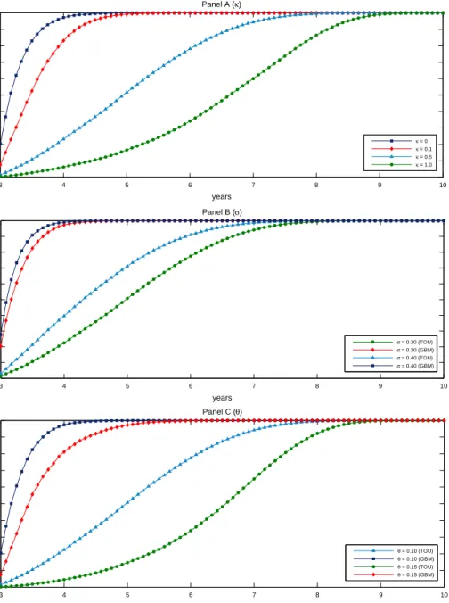
Panel A of Figure 4 represents 𝐹(𝑡) as a function of 𝜅. Clearly, as 𝜅 increases, this probability is lower for any date before the expiration date. Thus, in comparison with the GBM process, the executive always waits longer for exercising the ESO. Panel B depicts the case for different values of𝜎 when the stock price is driven by either a TOU or its equivalent GBM process. Generally, a higher volatility leads to earlier exercise (lower𝜏∗) and specifically when the level of predictability is low, as in a GBM process. A larger value of𝜎 means that i) the executive’s wealth becomes more volatile due to the ESOs but also because of the restricted stocks, and ii) the option may be deep in-the-money with a higher probability. Boths facts suppose an earlier exercise of the ESO, according to panel B findings. Finally,
Figure 4: Cumulative probabilities of early exercise. 3 4 5 6 7 8 9 10 0 0.1 0.2 0.3 0.4 0.5 0.6 0.7 0.8 0.9 1 years Cumulative probability Panel A (κ) 3 4 5 6 7 8 9 10 0 0.1 0.2 0.3 0.4 0.5 0.6 0.7 0.8 0.9 1 years Cumulative probability Panel B (σ) 3 4 5 6 7 8 9 10 0 0.1 0.2 0.3 0.4 0.5 0.6 0.7 0.8 0.9 1 years Cumulative probability Panel C (θ) κ = 0 κ = 0.1 κ = 0.5 κ = 1.0 σ = 0.30 (TOU) σ = 0.30 (GBM) σ = 0.40 (TOU) σ = 0.40 (GBM) θ = 0.10 (TOU) θ = 0.10 (GBM) θ = 0.15 (TOU) θ = 0.15 (GBM)
We plot the cumulative probabilities that the exercise time is not greater than some given date𝑡, 𝐹(
𝑡)
, for some values of 𝜅,𝜎 and 𝜃. Panel A shows the curves corresponding to 𝜅 = 0, 𝜅 = 0.10, 𝜅 = 0.50 and𝜅= 1.0. The remaining parameters have been set to𝜃= 0.10 and𝜎= 0.30. In panel B, the curves represent the cases𝜎 = 0.30 and𝜎 = 0.40, where the other parameters have been set to 𝜅= 0.50 and
𝜃= 0.10. Finally, in panel C the curves represent the cases𝜃= 0.10 and𝜃= 0.15 with the other parameters set to𝜅= 0.50 and𝜎= 0.30. For comparison purposes, we have also plotted the same probability for the corresponding equivalent GBM process described in Appendix A. The general finding is that, executives will tend to wait longer to exercise ESOs as the predictability of the process increases, that is, a higher value of
𝜌𝑟(1)
panel C shows the same situation for several values of 𝜃 and it does not deserve further comments.
3.3 The objective bias
In this subsection, we analyze the sign and size of the biases that can occur because of a misspecification of the underlying process for the stock price. As we have mentioned before, the literature has typically postulated a GBM process for the stock price. This assumption implies that the discrete-time returns will follow a white noise with drift. But, if the log-price were to follow a TOU process, as we have assumed in our computations, the discrete-time returns would follow an ARMA(1,1) process with trend. Thus, the firm’s cost𝑉𝑂𝐵𝐽 would be biased as a result of an erroneous choice for the stochastic process of the price dynamics. We designate this bias as12
𝐵𝑖𝑎𝑠1 =
𝑉𝑂𝐵𝐽
𝐹 −𝑉𝑂𝐵𝐽
𝑉𝑂𝐵𝐽 ×100 , (13)
where𝑉𝑂𝐵𝐽
𝐹 denotes the objective value computed under the false hypothesis that prices are driven by a GBM process. We maintain the notation 𝑉𝑂𝐵𝐽 to denote the objective value computed under the true process. We have calculated this bias for different values of𝜅 and the results are displayed in panel A of Figure 5. For 𝛾 = 2, the objective bias is generally positive and increasing with predictability. Note that the size of the bias is not high in this case, meanwhile for𝛾 = 4 the sign of the bias turns out to be negative and its size becomes quite substantial even for moderate degrees of undiversification.
The results of performing the same analysis but for different values of 𝜎 are depicted in panel B of Figure 5. We have found the same pattern described before, namely, when the executive has a low degree of relative risk-aversion and is well diversified, 𝑉𝑂𝐵𝐽
𝐹 tends to overstate the true cost but not much. As the degree of relative risk-aversion increases and the executive becomes worse diversified,𝑉𝑂𝐵𝐽
𝐹 understates the true cost in such a way that the size of the bias turns out to be above 10% for most values of𝜎.
We have also computed the objective bias for several alternative values of𝜃. The results
12
Notice that the objective value can be computed either using a conventional binomial model or, as we do, by using the LSM method. We illustrate the size of bias using this latter method, but the results should be similar with other methods of computing𝑉𝑂𝐵𝐽.
Figure 5: Objective ESO valuation bias under the S1 framework (S1),𝐵𝑖𝑎𝑠1 0.1 0.5 0.75 1 −20 −15 −10 −5 0 5 10 Panel A κ Bias 1 0.2 0.25 0.3 0.35 0.4 0.45 −20 −15 −10 −5 0 5 10 Panel B σ Bias 1 0.065 0.085 0.1 0.125 0.15 −20 −15 −10 −5 0 5 10 Panel C θ Bias 1 γ = 2; α = 1/2 γ = 2; α = 2/3 γ = 4; α = 1/2 γ = 4; α = 2/3
We plot the percentage bias in equation (13), which is incurred when the firm’s cost of a 10-year ESO with a vesting period of 3 years is evaluated using a GBM process for the stock price when the true one is a TOU process. Panels A to C depict this bias as a function of, respectively,𝜅,𝜎and𝜃, for four combinations of the relative degree of risk-aversion and the executive’s degree of undiversification. In all cases, we have set
are shown in panel C of Figure 5. Along the lines of the previous results, the sign of the bias is positive when the degree of risk-aversion is low and the executive is relatively well diversified. However, as the degree of risk-aversion increases and the executive becomes less well diversified, the sign of the bias becomes negative and its size is also well above 10% for almost all cases considered.
We can conclude that for high degrees of relative risk-aversion, the objective value assum-ing a GBM process can understate substantially the true firm’s ESO cost. Finally, the size of the bias does not appear to be significantly affected by the length of the vesting period and it has not been reported here.
4
The two state-variable framework
Here we explore how the executive’s exercise policy and hence, the ESO objective value is modified by including a market portfolio. This extended set-up is assumed to provide the true objective value,𝑉𝑂𝐵𝐽. We keep the benchmark values of the previous section for describing the environment of the representative executive as well as those describing the TOU process. The parameters characterizing the dynamics of the market portfolio are 𝜇𝑀 = 0.10 and 𝜎𝑀 = 0.20. The initial value of the market portfolio will be set to one and the correlation between the innovations in the stock and the market portfolio,𝜌, will be set to 0.50. Basically, to obtain𝑉𝑂𝐵𝐽
𝑆2 we solve the executive’s problem for a grid of values of 𝜂 in order to obtain
the value𝜂∗which maximizes the executive’s utility.13 This makes𝑆2 model more demanding in computational terms than the𝑆1 model, which doesn’t need finding𝜂∗.
The results are summarized in a ratio that measures the difference between the objective value in the one state-variable model,𝑉𝑂𝐵𝐽
𝑆1 , and the objective value in the two state-variable
model,𝑉𝑂𝐵𝐽
𝑆2 , as a percentage of the latter. Hence,
𝐵𝑖𝑎𝑠2 = 𝑉𝑂𝐵𝐽 𝑆1 −𝑉𝑆𝑂𝐵𝐽2 𝑉𝑂𝐵𝐽 𝑆2 ×100 . (14) Recall that𝑉𝑂𝐵𝐽
𝑆2 measures the true cost of ESOs for firms. Cai and Vijh (2005) have shown
that this ratio is positive when the stock price is driven by a GBM process. The reason is that,
13
Table 3: Predictability and ESO cost: S1 versus S2 models. 𝜅 𝜈 𝛼 0.05 0.10 0.25 0.50 1.00 0 1/2 13.34 8.16 1.41 -0.24 -0.62 2/3 19.93 13.29 3.11 0.46 -0.34 3 1/2 8.99 6.80 1.01 -0.07 -0.53 2/3 10.02 8.14 2.62 0.44 -0.31
We present here for𝛾 = 4 the percentage bias defined in equation (14), concerning the firm’s ESO cost when executives have available a market portfolio to allocate their unrestricted wealth (S2 model) against the case in which they have not (S1 model). As it is shown, the differences decrease as
𝜅increases to become negligible for relatively high values of this parameter. For the rest of the parameters see Table 2 and Section 4.
under model S1, executives can allocate their unrestricted wealth only in the risk-free asset whereas under model S2, they can also invest in the market portfolio. Since this alternative becomes more attractive, the average exercise times will be generally lower in the S2 model. Our results are presented in Table 3. We have restricted our attention on the impact of changes in predictability, so that we only report the results concerning changes in𝜅. In this regard, we have maintained our choice of adjusting𝜎 such that the volatility of discrete-time stock returns is not affected.
For the case of 𝛾 = 4,𝑉𝑂𝐵𝐽 increases with 𝜅 in both S1 and S2 models.14 For 𝜅≥0.25,
which implies a first order autocorrelation higher than 0.0103 in absolute value, the firm’s ESO cost for both models becomes indistinguishable. To get some intuition for this result, recall that the market portfolio is driven by a GBM process. Then, when executives observe a higher predictability in the firm’s stock returns, they do not see any advantage in exercising earlier to place the proceeds into the market portfolio. As a result, the average exercise time and the threshold price are essentially the same in both the S1 and the S2 models. This result becomes quite relevant to the extent that 𝑉𝑂𝐵𝐽
𝑆1 can be obtained at a lower computational
costs than𝑉𝑂𝐵𝐽 𝑆2 .
Finally, we have also studied how the share of the market portfolio is affected by changing
14
ESO cost for firms behaves differently when𝛾= 2. In the S1 model, 𝑉𝑂𝐵𝐽 decreases with𝜅. In the S2
model,𝑉𝑂𝐵𝐽 increases with𝜅. However the behavior of the percentage bias is completely analogous, namely,
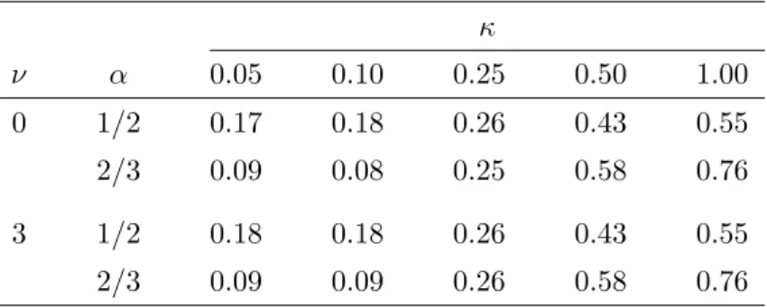
Table 4: Optimal share of market portfolio (𝜂∗). 𝜅 𝜈 𝛼 0.05 0.10 0.25 0.50 1.00 0 1/2 0.17 0.18 0.26 0.43 0.55 2/3 0.09 0.08 0.25 0.58 0.76 3 1/2 0.18 0.18 0.26 0.43 0.55 2/3 0.09 0.09 0.26 0.58 0.76
The table displays, for 𝛾 = 4, how 𝜂∗ is affected by a higher
pre-dictability of the firm’s stock returns. The volatility of stock returns in discrete-time is kept constant.
the predictability of the firm’s stock returns. The results are displayed in Table 4, which focuses on the impact of different values of 𝜅 and distinguishes between the 3-year vesting and the no vesting cases. It is shown that a greater predictability leads the executive to put more wealth in the market portfolio and less into the risk-free asset. In fact, the executive puts even more weight in the market portfolio for a higher undiversification level, 𝛼, when the predictability of the stock returns is above a specific threshold (see the last two columns in Table 4). Note that this pattern is independent of the vesting period length.
We have seen that a greater predictability in stock returns leads executives to hold a higher share of their unrestricted wealth in the market portfolio and also to wait longer for exercising the ESOs. From an intertemporal point of view, this means that executives are substituting their holdings of the risk-free asset by ESOs because of their higher expected return, which is subject to less uncertainty as predictability increases.
5
The FAS 123R bias
As a result of the increasing relevance of ESOs in managers’ compensation packages, the International Financial Reporting Standard (IFRS) and the Financial Accounting Standards Board (FASB) have issued several requirements for a fair valuation of those expenses. Both standards require to consider the same factors to obtain the fair value: the market price of the shares, the exercise price of the options, the risk-free interest rate, the expected volatility of stock prices, the expected dividend on stock and the number of years until options expire.
However, there are some differences between both standards. The main accountant dif-ference concerns the classification of the award as a liability or equity. Following FAS 123R, if there exists a possibility to settle the award in cash, it is always classified as a liability award, meanwhile IFRS 2 classification is based on the method of expected settlement (cash or shares), that is, the possibility of cash settlement does not imply a liability award. Other minor differences concern the definition of grant date and the vesting period effects. For instance, the IFRS 2 establishes the grant date when the agreement is reached, but under the FAS 123R the grant date is the earlier between the mutual understanding date and the date when employee begins to provide his services. As regards the vesting period, when account-ing for ESO plans with graded vestaccount-ing under the ”European” standard (IFRS 2), we must treat each tranche as a separate award while under the FAS 123R we can use a straight-line method for the entire award.
Notice that the above differences do affect accountant practice but not the concept of fair value. Thus, the fair value is the same under both standards, independently of which one is followed to account for the expense. Furthermore, both provide similar recommendations for computing the fair value and, as a matter of choice, we have selected FASB’s recommendations to compare our model with these suggestions.
In its Financial Accounting Standard Board (2004) No 123 revised statement (FAS 123R), the FASB requires firms to disclose the method used to estimate the grant-date fair value of their ESO compensation packages. Among the valuation techniques that the FAS 123R considers acceptable, it appears as candidates both the BS and binomial models. The BS formula is appealing because of its simplicity. However, there are some features of ESOs that are not well captured by using this formula. In particular, the BS model assumes European-style options whereas ESOs are typically American options that executives tend to exercise before maturity, see Bettis et al. (2005). To consider this fact, the FAS 123R (paragraph A26) explicitly requires computing this fair value by replacing the ESO expiration date,𝑇, with its expected exercise time, or expected life, 𝜏∗. Specifically, the ESO price should be
calculated as
𝑉𝐹 𝐴𝑆 =𝐵𝑆(
𝜏∗)
. (15)
two possibilities in this regard. First, the firm can use historical data about the executives’ exercise behavior. Alternatively, the early exercise can be described using some binomial model that, by capturing the executives’ exercise policy, determines the ESO’s expected life, the required input in the BS model.
Kulatilaka and Marcus (1994), argue that the FAS123 proposal may yield a biased es-timation of the firm’s ESO costs if historical data are used to estimate 𝜏∗, because these historical data are only one particular realization of stock prices. However, Carpenter (1998) compares the performance of three alternatives models, an utility-maximizing model, an ex-tended American option model, in which she introduces an exogenous stopping rate, and the FAS 123 proposal. She obtains that the three alternatives yield similar values for the ESO cost when the models are calibrated to yield the same executive’s exercise policy. Am-mann and Seiz (2004) also compare similar alternative models to compute the ESO fair value. They clearly show that the expected life of the ESO is the key variable underlying the models, and that pricing differences become negligible when the models are calibrated to the same expected life of the option.
In any case, and independently of the model used to obtain the executive’s exercise policy, our contention is simply that firms typically assume that stock prices are driven by a GBM process. If the true model is a TOU process, the resulting executive’s exercise policy is flawed and the implied average exercise date would be biased, leading also to a biased fair value.
Therefore, it is interesting to compare the firm’s ESO cost under the TOU process,𝑉𝑂𝐵𝐽, with the BS value obtained under the erroneous DGP that prices are driven by a GBM process, 𝐵𝑆(𝜏𝐹∗), where 𝜏𝐹∗ denotes its corresponding expected life. Specifically, we will analyze the following percentage bias:
𝐵𝑖𝑎𝑠3 =
𝐵𝑆(𝜏𝐹∗)−𝑉𝑂𝐵𝐽
𝑉𝑂𝐵𝐽 ×100. (16)
We have focused on the behavior of this bias for different values of the parameter 𝜅. We have taken as𝜏∗
𝐹 the value for the case of 𝜅 = 0, which is the equivalent GBM process for the stock price. Furthermore, the volatility of the discrete-time returns, 𝜎𝑟, has been kept constant by a suitable adjustment of the diffusion coefficient,𝜎, as in Section 3. As a result, the appropriate value of the firm’s stock return volatility to be plugged into the BS formula
Figure 6: FAS123 bias. The one state-variable framework. 0.1 0.25 0.5 0.75 1 −40 −35 −30 −25 −20 −15 −10 −5 No vesting κ Bias 3 0.1 0.25 0.5 0.75 1 −40 −35 −30 −25 −20 −15 −10 −5 Vesting = 3 years κ Bias 3 γ = 2; α = 1/2 γ = 2; α = 2/3 γ = 4; α = 1/2 γ = 4; α = 2/3
We plot the percentage bias defined in equation (16), which is incurred when the FAS123 procedure is used and the expected life of the ESO is computed using erroneously the GBM process instead of the TOU process for stock returns. Both TOU and GBM have been made comparable by equalizing their means and volatilities. The procedure is described in detail in Section 5. The values of the remaining parameters are: 𝑟𝑓 = 0.06, ¯𝑞= 0 and𝑇 = 10.
is 30% for all values of𝜅. In our analysis we have assumed a 10-year ESO for the cases of no vesting and a 3-year vesting period. The results are depicted in Figure 6 for the S1 model.
We can see that the bias is generally negative. Hence, the estimation of the ESO expected life using a GBM process for the stock price, when TOU is the true process, understates the true expected cost systematically. This result is related to the behavior of the expected exercise date already discussed in subsection 3.1. We have shown that executives tend to wait longer for exercising ESOs when predictability increases, so that the lowest 𝜏∗ is achieved when 𝜅 = 0. This, in turn, implies a low BS value for the ESO in comparison with the firm’s ESO cost under the TOU process. We show that the size of this bias increases with the predictability of the process for𝛾 = 2, but decreases for𝛾 = 4. This is explained by the different behavior of𝑉𝑂𝐵𝐽 for each value of the relative risk-aversion parameter.
We end this section by reporting briefly the results for the FAS bias when the S2 model is considered. By using a similar procedure to that described for the S1 model, we find that the inclusion of a market index only increases the undervaluation incurred when the FAS123 recommendations are used.
6
Conclusions
We have shown that predictability matters for valuing American ESOs from the firm’s per-spective. The objective value, or firm’s ESO cost, is biased if one assumes erroneously that stock prices are driven by a geometric Brownian motion (GBM) instead of the true process driven by a trending Ornstein-Uhlenbeck (TOU) process. This bias is significant even for rel-atively low values of the first order autocorrelations. The executive performs his ESO exercise under two alternative asset menu settings. One of them consists only of the risk-free asset and the other one is extended by including also the market portfolio. When predictability increases, the pricing differences between both approaches vanish. Moreover, independently of the executive’s wealth composition, he waits longer for the ESO exercise the higher the predictability. Finally, we examine the consequences of predictability for the FAS123 propos-als. When the erroneous GBM process is used for prices, it generates an undervaluation of the firm’s ESO cost, even for moderate low levels of predictability.
Some important extensions for future research are suggested next. First, it would be interesting to analyze the executive’s asset allocation problem, when there is the possibility of reallocating the market portfolio along the planning horizon (dynamic allocation) as in Barberis (2000), jointly with holding American ESOs. The quadratic approximation for the valuation of ESOs can be a good candidate to make easier its implementation. See, for instance, Kimura (2010). Finally, it would be also interesting to introduce the executive forfeiture and the case of perpetual options into our framework. See again Kimura (2010) and also, Jennergren and N¨aslund (1996) among others.
References
Ammann, M., Seiz, R., 2004. Valuing employee stock options. Does the model matter? Fi-nancial Analysts Journal 60 (5), 21–37.
Barberis, N. C., 2000. Investing for the long run when returns are predictable. The Journal of Finance 55 (1), 225–264.
Bergstrom, A. R., 1984. Handbook of Econometrics. Vol. 20. North Holland, Amsterdam, Ch. Continuous time stochastic models and issues of aggregation over time, pp. 1145–1212.
Bettis, J. C., Bizjak, J. M., Lemmon, M. L., 2005. Exercise behavior, valuation, and the incentive effects of employee stock options. Journal of Financial Economics 76 (2), 445– 470.
Bouchard, B., Warin, X., 2011. Monte-Carlo valorisation of american option: facts and new algorithms to improve existing methods. Numerical Methods in Finance, ed. R. Carmona, P. Del Moral, P. Hu and N. Oudjane,Springer Proceedings in Mathematics.
Brockwell, P., 2001. Handbook of Statistics. Elsevier Science, Amsterdam, Ch. Continuous-time ARMA processes.
Brown, P., Szimayer, A., 2008. Valuing executive stock options: Performance hurdles, early exercise and stochastic volatility. Accounting and Finance 48, 363–389.
Cai, J., Vijh, A. M., 2005. Executive stock and option valuation in a two state-variable framework. Journal of Derivatives 12 (3), 9–27.
Campbell, J. Y., Lo, A. W., Mackinlay, A., 1997. The Econometrics of Financial Markets. Princeton, Princeton University Press.
Campbell, J. Y., Yogo, M., 2006. Efficient tests of stock return predictability. Journal of Financial Economics 81, 27–60.
Carpenter, J. N., 1998. The exercise and valuation of executive stock options. Journal of Financial Economics 48 (2), 127–158.
Duan, J.-C., 1995. The GARCH option pricing model. Mathematical Finance 5, 13–32.
Financial Accounting Standard Board, 2004. Statement of financial accounting standards no 123 (revised 2004): Share-based payments. FASB.
Grundy, B. D., 1991. Option prices and the underlying asset’s return distribution. Journal of Finance 46, 1045–1069.
Hafner, C. M., Herwartz, H., 2001. Option pricing under linear autoregressive dynamics, heteroskedasticity, and conditional leptokurtosis. Journal of Empirical Finance 8, 1–34.
Hall, B. J., Murphy, K. J., 2002. Stock options for undiversified executives. Journal of Ac-counting and Economics 33 (1), 3–42.
Huang, Y.-C., Wu, C.-W., Wang, C.-W., 2009. Valuing American options under ARMA processes. International Research Journal of Finance and Economics 28, 152–159.
Ingersoll, J. E., 2006. The subjective and objective evaluation of incentive stock options. Journal of Business 79 (2), 453–487.
Jennergren, L. P., N¨aslund, B., 1996. A class of options with stochastic lives and an extension of the black-scholes formula. European Journal of Operational Research 91, 229–234.
Jokivuolle, E., 1998. Pricing European options on autocorrelated indexes. Journal of Deriva-tives 6, 39–52.
Kimura, T., 2010. Valuing executive stock options: A quadratic approximation. European Journal of Operational Research 207, 1368–1379.
Kulatilaka, N., Marcus, A. J., 1994. Valuing employee stock options. Financial Analysts Journal 50 (6), 46–56.
Lambert, R. A., Larcker, D. F., Verrecchia, R. E., 1991. Portfolio considerations in valuing executive compensation. Journal of Accounting Research 29 (1), 129–149.
Le´on, A., Vaello-Sebasti`a, A., 2009. American GARCH employee stock option valuation. Journal of Banking and Finance 33 (6), 1129–1143.
Le´on, A., Vaello-Sebasti`a, A., 2010. A simulation-based algorithm for American executive stock option valuation. Finance Research Letters 7, 14–23.
Liao, S.-L., Chen, C.-C., 2006. The valuation of European options when asset returns are autocorrelated. The Journal of Futures Markets 26 (1), 85–102.
Lo, A., Wang, J., 1995. Implementing option pricing models when returns are predictable. The Journal of Finance 50 (1), 87–129.
Longstaff, F., Schwartz, E., 2001. Valuing American options by simulation: A simple least-squares approach. Review of Financial Studies 14 (1), 113–147.
Moreno, M., Navas, J. F., 2003. On the robustness of least-squares Monte Carlo (LSM) for pricing American derivatives. Review of Derivatives Research 6 (2), 107–128.
Paschke, R., Prokopczusk, M., 2010. Commodity derivative valuation with autoregressive and moving average components in the price dynamics. Journal of Banking and Finance 34, 2742–2752.
Poterba, J. M., Summers, L. H., 1988. Mean reversion in stock prices. Journal of Financial Economics 22, 27–59.
Stentoft, L., 2004. Assessing the least squares Monte-Carlo approach to American option valuation. Review of Derivatives Research 7, 129–168.
Taylor, S. J., 2005. Asset Price Dynamics, Volatility and Prediction. Princeton University Press.
Tian, Y. S., 2004. Too much of a good incentive? the case of executive stock options. Journal of Banking and Finance 28, 1225–1245.
Yiang, G. J., Tian, Y. S., 2010. Forecasting volatility using long memory and comovements: An application to option valuation under SFAS 123R. Journal of Financial and Quantitative Analysis 45 (2), 503–533.
Appendix A.ARMA representation of exact discretization of TOU process.
We rewrite equation (5) in terms of the detrended process of𝑝𝑡:
𝑑𝑞𝑡=−𝜅𝑞𝑡𝑑𝑡+𝜎𝑑𝑍𝑆,𝑡, 𝜅 >0
where𝑞𝑡≡𝑝𝑡−𝜃𝑡and initial condition 𝑞0 =𝑝0 = ln𝑆0. The exact solution to this univariate
Ornstein Uhlenbeck (OU) process reverting to an unconditional mean of zero is, according to Bergstrom (1984), the following discrete-time process:
𝑞𝑡=𝑓ℎ𝑞𝑡−ℎ+𝜀𝑡, 𝜀𝑡∼ iid 𝑁(0, 𝜎2𝜀,ℎ ) where𝑓ℎ ≡ 𝑒−𝜅ℎ <1 and 𝜎2𝜀,ℎ = 𝜎2 2𝜅 ( 1−𝑒−2𝜅ℎ)
. Next, we obtain the equation for Δℎ𝑞𝑡 ≡ 𝑞𝑡−𝑞𝑡−ℎ and rewrite in terms of the stock return, 𝑟𝑡,ℎ, given in equation (10). Then,
𝑟𝑡,ℎ =𝜃ℎ
(
1−𝑓ℎ
)
+𝑓ℎ𝑟𝑡−ℎ,ℎ+𝜂𝑡, 𝜂𝑡=𝜀𝑡−𝜀𝑡−ℎ,
where𝜂𝑡 follows a MA(1) process verifying that
E[𝜂𝑡] = 0, Var(𝜂𝑡) = 2𝜎𝜀,ℎ2 and Cov(𝜂𝑡, 𝜂𝑡−𝑗ℎ) =
⎧ ⎨ ⎩ −𝜎2 𝜀,ℎ if𝑗= 1 0 if𝑗≥2
Hence, 𝑟𝑡,ℎ is described by a stationary discrete-time ARMA (1,1) process with an uncon-ditional mean of 𝜃ℎ, an unconditional variance 𝜎2𝑟 shown in equation (11) and a negative first-order autocorrelation 𝜌𝑟(1) exhibited in equation (12). Finally, the returns are nega-tively correlated at all lags. The higher order autocorrelation coefficients are easily obtained as𝜌𝑟(𝑗) =𝑓ℎ𝑗−1𝜌𝑟(1), ∀𝑗≥2.
The following table summarizes the moments of the continuously compounded returns, defined as in equation (10) under the two alternative processes.
TOU GBM Mean (¯𝑟) 𝜃ℎ ( ˜ 𝜇−𝜎˜2/2) ℎ Variance (𝜎𝑟,ℎ2 ) 𝜎 2 𝜅 ( 1−𝑒−𝜅ℎ) ˜ 𝜎2ℎ Autocorrelation at lag 1 −1 2 ( 1−𝑒−𝜅ℎ) 0 ˜
𝜇and ˜𝜎denote the trend and diffusion coefficients of the GBM process.
By matching both unconditional means and variances for the h-period returns under both processes, we obtain the following constraints in the parameters:
˜ 𝜇=𝜃+𝜎˜ 2 2 , 𝜎˜=𝜎 √ 1−𝑒−𝜅ℎ 𝜅ℎ .
In short, these parameter restrictions lead to a fair comparison across the paper when we aim to analyze exclusively the effects of predictability on the objective ESO valuation.
Appendix B.Subjective and objective ESO pricing algorithm.
The algorithm used to solve the executive’s problem in equation (7) is based on the popular LSM algorithm of Longstaff and Schwartz (2001) for valuing American options. The modification to consider a risk-averse option holder was introduced by Le´on and Vaello-Sebasti`a (2010). We really adapt this approach, summarized in steps 1 to 6 below, by changing the dynamics of the stock price process. Given𝑚 simulated paths, the algorithm consists on creating a vector𝑌 of length 𝑚with the expected utility for each path obtained from the optimal exercise of the ESOs. For the one state-variable case (𝑆1) the algorithm simplifies, since the executive only has to search the optimal exercise time,𝑡∗ (𝜂= 0). Then, we first explain the algorithm for the𝑆1 model and later, we will extend it for the 𝑆2 case.
Step 1: Given𝑚simulated paths of the state-variable (𝑆𝑡), the optimal exercise rule at maturity (𝑇) is obvious, to exercise all paths in-the-money. Vector𝑌𝑇 is obtained using equations (1) and (6) on all paths at 𝑇.
Step 2: At 𝑇 −1 the executive has to choose between exercising or continuing with the ESOs for one period. The utility at 𝑇 in case of exercise at 𝑇−1,𝑈(
𝑊𝑇∣𝑇−1)
using equations (2) and (6). Finally, to estimate the expected utility of exercise condi-tional on the current values of the state-variables,E𝑇−1
[ 𝑈( 𝑊𝑇∣𝑇−1 ) ∣𝑆𝑇−1 ] , we regress 𝑈( 𝑊𝑇∣𝑇−1 )
over some basis functions of the state-variable (𝑆𝑇−1). The projected
val-ues of that regression are ˆE𝑇−1
[ 𝑈( 𝑊𝑇∣𝑇−1 ) ∣𝑆𝑇−1 ] .
Step 3: Compute the expected utility in case of keeping the ESO one period ahead. We only have to regress the one period ahead utility, 𝑌𝑇, over basis functions of 𝑆𝑇−1. Then
ˆ
E𝑇−1[𝑌𝑇∣𝑆𝑇−1] is the projected value of the previous regression.
Step 4: Compare the expected utility when exercising and holding the ESOs and then, select the maximum. That is, we compare ˆE𝑇−1[𝑈(𝑊𝑇∣𝑇−1
)
∣𝑆𝑇−1](step 2) with ˆE𝑇−1[𝑌𝑇∣𝑆𝑇−1]
(step 3). For those 𝑦 paths where ˆE𝑇−1
[ 𝑈( 𝑊𝑇∣𝑇−1 ) ∣𝑆𝑇−1 ] > Eˆ𝑇−1[𝑌𝑇∣𝑆𝑇−1] the
ESOs are exercised and the𝑦elements of𝑌𝑇 are updated with ˆE𝑇−1
[ 𝑈( 𝑊𝑇∣𝑇−1 ) ∣𝑆𝑇−1 ] .
Step 5: Repeat steps 2 to 4 up to𝑡0, where𝑡0 can be either the grant date or the first time step
after the vesting period, and compute the expected utility as the mean of𝑌𝑇.
Step 6: Find the certainty-equivalence using equations (8) and (17).
To compute the expectations at steps 2 and 3 we must select the basis functions. We have noticed that the algorithm works better when using powers of log(𝑆𝑡) instead of powers of 𝑆𝑡, specifically we use log(𝑆𝑡), [log(𝑆𝑡)]2 and [log(𝑆𝑡)]3. Regarding the number of basis functions, adding higher order powers yields less stable results because the matrix of basis functions becomes close to singular. This yields less accurate results when computing the inverse.15
To obtain the firm’s ESO cost𝑉𝑂𝐵𝐽, we follow the approach of Hall and Murphy (2002), which is based on the exercise threshold. This threshold establishes a frontier where the executive is indifferent between holding or exercising the option. Thus, if the stock price is above (below) the frontier, the executive will exercise (hold) the ESO.
To compute the exercise threshold, at step 4 in the previous algorithm, we record the minimum value of𝑆𝑡 for which the executive decides to exercise the ESO. Once we have
ob-15
Moreno and Navas (2003) and Stentoft (2004) provide numerical details about the robustness of the LSM method. New Monte-Carlo type methods, based on either the Malliavin calculus or the regression based approaches, to improve the efficiency for the pricing of American options can be found in Bouchard and Warin (2011).