Optimising a Mining Portfolio Using CVaR
By
D. E. Allen, A. R. Kramadibrata, R. J. Powell and A. K. Singh
School of Accounting, Finance and Economics, Edith Cowan University
School of Accounting, Finance and Economics & FEMARC Working Paper Series Edith Cowan University
November 2011 Working Paper 1106
Correspondence author: Akhmad R. Kramadibrata
School of Accounting, Finance and Economics Faculty of Business and Law
Edith Cowan University Joondalup, WA 6027 Australia
Phone: +618 6304 5265 Fax: +618 6304 5271
ABSTRACT
The mining industry can be extremely volatile during times of economic downturn. We compare extreme risk in mining share portfolios from each of the world’s seven leading mining areas using Conditional Value at Risk (CVaR) which measures those risks beyond traditional Value at Risk (VaR) metrics. We also show how CVaR can be used to optimise portfolios and minimise extreme risk. We find significant differences between countries in CVaR as compared to standard deviation risk rankings, as well as differences in portfolios optimised using CVaR compared to portfolios using traditional variance methodology. This indicates that investors will not adequately minimise risk using traditional approaches.
Keywords: Value at risk; Conditional value at risk; Mining share portfolios
Acknowledgements: The authors would like to thank the Australian Research for funding support.
1
1. Introduction
The mining industry can be highly volatile in times of extreme economic downturn. Most metals & mineral commodities and share markets showed strong growth and relatively low volatility in the period from 2002 to 2006, leading up to the Global Financial Crisis (GFC). These commodities and share markets then entered a period of extreme volatility with very high growth during most of 2007, followed by sharp declines with prices falling by half between July 2008 and January 2009 (World Bank, 2011b). Thereafter a very sharp upward trend was resumed for the remainder of 2009, with many of these commodities regaining (and in many cases, surpassing) their pre-GFC prices. To distinguish between these two periods of distinctly different volatility, we will hereafter refer to the 2000-2006 period as the low volatility (LV) period, and to 2007-2009 as the high volatility (HV) period. Mining companies have been shown to have deteriorated further than most other industries during the Global Financial Crisis (GFC) in regards to both market and credit risk (Allen, Powell, & Singh, 2011; Powell & Allen, 2009). Given this scenario, it is important for investors to understand extreme risk in this sector in share portfolio allocation.
Conditional Value at Risk (CVaR) is a metric which measures extreme tail risk – that risk which lies beyond traditional standard deviation and Value at Risk (VaR) measures. Using CVaR, we compare share price volatility in the most mining intensive countries for the LV and HV periods to answer four research questions. First, which countries display the highest (lowest) extreme risk? Second, does relative risk between these countries change over the HV period as compared to the LV period? Third, is relative risk different using CVaR as compared to standard deviation? Fourth, we show how to optimise a mining portfolio using CVaR and determine whether this is significantly different to using a traditional Markowitz (1952) standard deviation approach.
We find that maximum returns are obtainable from South America during the LV period and China during the HV period. CVaR is minimised in both periods with high weightings in Australian, Chinese and Russian stocks. We also found that relative risk between countries is significantly different using CVaR as compared to standard deviation, leading to differences in optimal portfolio mix.
The next section of the paper provides a literature survey and background information on the mining industry, CVaR and portfolio optimisation. Section 3 deals with data and methodology. Section 4 covers the findings and discussion, with conclusions and implications provided in Section 5.
2. Background and Literature Review
2.1. The Global Resources Industry
The global mining industry is dominated by Australia, Canada, China, Russia, South Africa, South America (predominantly Chile) and the USA. Australia is one of the world’s largest metals and minerals producers, with substantial production of a wide range of commodities such as bauxite, iron ore, gold, lead nickel, silver,
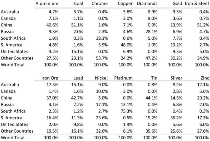
2 zinc and zircon. Canada has substantial production of a range of metals and minerals such as aluminium, diamonds, gold and nickel. China leads the world in the production of several commodities, producing more than 40% of the world’s aluminium, coal, iron & steel, lead and tin, as well as producing a wide range of other commodities. South Africa produces a wide range of metals and minerals, leading the world in chrome and platinum and has one of the world’s largest gold reserves. Chile leads the world’s copper production. Russia is one of the world’s largest producers of diamonds and also produces a significant portion of global crude oil, gold nickel, platinum and silver. The USA is a major producer of a wide range of commodities, including coal, gold and silver. Table 1 summarises the world market share of key resources.
Table 1. Global Mining Market Share
Sources: (British Geological Survey, 2011; International Energy Agency, 2011; MBendi Information Services, 2011; U.S. Geological Survey, 2011).
Strong growth in global demand for resources has been fuelled largely by demand from resource hungry China. who has experienced a rapidly expanding economy for three decades, with growth in GDP averaging 9.6% for this period(World Bank, 2011a). China consumes almost all their own resource production and is the world’s largest importer of minerals. Their demand includes two thirds of the worlds iron ore production, almost half of the world’s coal production, as well as a wide range of other metal and minerals (U.S. Geological Survey, 2011). China’s demand for resources is in turn being driven by factors such as world demand for
Aluminium Coal Chrome Copper Diamonds Gold Iron & Steel Australia 4.7% 5.7% 0.4% 5.6% 8.9% 9.3% 0.4% Canada 7.1% 1.1% 0.0% 3.0% 9.0% 3.6% 0.7% China 40.6% 51.1% 1.6% 7.1% 0.9% 13.9% 51.2% Russia 9.3% 2.0% 2.3% 4.6% 28.1% 6.9% 4.7% South Africa 1.9% 0.3% 38.1% 0.6% 5.0% 7.7% 0.4% S. America 4.8% 1.6% 3.9% 48.0% 1.0% 19.2% 2.7% United States 4.2% 15.1% 0.0% 6.9% 0.0% 9.3% 5.0% Other Countries 27.5% 23.1% 53.7% 24.2% 47.2% 30.2% 34.9% World Total 100.0% 100.0% 100.0% 100.0% 100.0% 100.0% 100.0% Iron Ore Lead Nickel Platinum Tin Silver Zinc Australia 17.3% 15.1% 9.0% 0.0% 0.8% 8.2% 12.1% Canada 1.4% 1.6% 10.0% 3.0% 0.0% 2.8% 5.6% China 37.0% 42.7% 5.0% 0.0% 44.1% 14.5% 29.2% Russia 4.1% 2.2% 17.1% 13.1% 0.4% 6.8% 2.0% South Africa 2.3% 1.2% 2.7% 75.3% 0.0% 0.4% 0.3% S. America 16.4% 11.3% 23.6% 0.5% 19.2% 36.2% 17.3% United States 2.0% 9.8% 0.0% 1.9% 0.0% 5.6% 6.0% Other Countries 19.5% 16.1% 32.6% 6.1% 35.6% 25.6% 27.6% World Total 100.0% 100.0% 100.0% 100.0% 100.0% 100.0% 100.0%
3 low cost Chinese manufacturing exports (Roberts & Rush, 2010) as well as internal factors such as consumption and investment (He & Zhang, 2010).
2.2. CVaR
Value at Risk (VaR) is a widely used metric for the measurement of market risk, measuring potential losses over a specified period at a specified confidence level. A key criticism of VaR is that it says nothing of the risks beyond the threshold measurement (for example, Samanta, Azarchs, & Hill, 2005). In addition, VaR has been found to be a non-coherent measure, having undesirable mathematical characteristics such lack of subadditivity (Artzner, Delbaen, Eber, & Heath, 1997, 1999) .
CVaR, on the other hand, measures risks beyond VaR, and has also been found to be a coherent measure, not having the undesirable characteristics of VaR (Pflug, 2000). If we are measuring VaR at a specified confidence level (β), then CVaR is the average of those risks beyond β, i.e. CVaR is the mean value of the worst (1- β)*100% losses. VaR is normally measured at high confidence intervals such as 95% or 99%. If, for example, we are measuring VaR at a 95% confidence level (β=0.95), CVaR is the average of the 5% worst losses.
2.3. Portfolio
Optimisation
The Markowitz (1952) portfolio optimisation approach generates a frontier (as per figure 1) which shows the most efficient combination of risk and return, with risk measured as the standard deviation (σ) of portfolio returns. As the frontier shows the maximum possible returns at each level of risk, σ-return combinations beyond the frontier are not possible and combinations below the frontier are inefficient. In order to capture extreme risk, our approach uses CVaR-return instead of σ-return as an optimisation tool. Use of CVaR as an optimiser in the literature is extremely limited with examples including credit portfolio optimisation (Andersson, Mausser, Rosen, & Uryasev, 2000) and Australian sectoral risk optimisation by the current authors (Allen & Powell, 2011).
3. Methodology
Using Datastream, we obtain ten years of daily price data to calculate CVaR and returns for individual mining companies in each of the key mining areas of Australia, Canada, China, Russia, South Africa, South America and the USA. We use a maximum of 30 mining companies in each area (the 30 largest by market capitalisation). These companies are identified from leading mining indices in each of the areas, including the Datastream and FTSE mining indices for each area as well as the S&P/ASX 300 Resources Index (Australia), S&P/TSX Comp Metals & Mining Index (Canada), FTSE Xinhua 600 Mining Index (China), FTSE/Russia Basic Materials Index (Russia, and the FTSE/JSE Resource Index (South Africa). This provides us with a total of 161 companies comprising the following number of companies in each area: Australia 30, Canada 30, China 30, Russia 7, South Africa 23, South America 11 and US 30.
4 There are a number of different techniques for measuring VaR and CVaR. We use a 95% historical approach which sorts historical returns from best to worst, with CVaR being the average of the worst 5% of returns. We divide our ten years of data into two periods, as discussed in the introduction, with Low Volatility (LV) being the years between 2000-2006 and High Volatility (HV) the years between 2007-2009. We calculate standard deviation, CVaR and returns for each entity for both periods. We then calculate country returns as the market capitalisation-weighted average returns of the individual companies in each country, and country CVaR being the weighted average of the individual company CVaRs. These are shown in Table 2.
To allow comparison between a traditional Markowitz variance-return approach and our CVaR-return approach, we calculate efficient frontiers based on both methods. To construct the σ-return frontier, we construct a variance-covariance matrix to account for correlation between our country returns, from which portfolio return and portfolio σ is calculated. The portfolio is then optimised to achieve the combination of assets yielding the minimum risk for each selected return level:
min ∑ ∑ (1)
Subject to
∑ 1 (2)
∑ IE (3)
0 (4)
where xi are portfolio weights, ri is the rate of return of industry sectors i and k, rp is the expected return on the portfolio and σik is the covariance between returns of industry sectors i and k (and similarly for all other industry sectors). Weighting for any portfolio cannot be negative, and can also be constrained to not exceed a specific weighting v (in order to ensure the portfolio is diversified).
For our CVaR-return frontier, we apply the same approach as above, except we use the standard deviation of the worst 5% of returns instead of the standard deviation of all returns. Our optimum σ-return (or CVaR-return) portfolio shows the combination of assets that yield the minimum portfolio σ (or CVaR) for each selected level of return. Our maximum return point is the highest return that can be generated by any country portfolio. The minimum return point is the return associated with the lowest possible σ (or CVaR). We select eight equidistant points between minimum and maximum returns (giving a total of 10 return points) and calculate the minimum portfolio σ or CVaR associated with each point. These
σ-return and CVaR-return combinations make up the efficient frontier, which we generate for the LV and HV periods.
5
3.1. Findings and Discussion
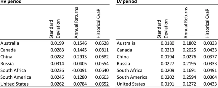
Table 2 shows the standard deviation and CVaR risk measures and the returns for each country’s mining portfolio. Rankings are shown in Table 4.
Table 2. Standard Deviation, Annual Returns and CVaR
Standard deviation and CVaR are daily average figures for the period. CVaR is the average of the worst 5% of returns as per the methodology section. The HV category is the 3 years from 2007-2009, while the LV is the 7 years from 2000 to 2006.
Both periods generally show positive returns, but different volatilities, especially using CVaR. Whilst the LV period was generally a period of sustained growth, the HV period was one of high growth, high decline, then high growth again. To better understand the HV period, a more comprehensive breakdown of returns during this time is shown in table 3. Most countries experienced strong growth in 2007, particularly China. The exception was South Africa with a small negative return. In 2009, Australia, Canada, South America and the US all gained more than they lost in 2008 in an impressive turnaround. Although China and Russia had exceptionally strong negative returns in 2008, they both showed an overall increase during HV due to the strong growth in 2007 and 2009.
HV period LV period St an d ar d De vi at io n A n nua l Re tu rn s Hi st o ri ca l Cv aR St an d ar d De vi at io n A n nua l Re tu rn s Hi st o ri ca l Cv aR Australia 0.0199 0.1546 0.0528 Australia 0.0180 0.1802 0.0333 Canada 0.0283 0.1445 0.0811 Canada 0.0213 0.2025 0.0433 China 0.0282 0.2913 0.0682 China 0.0194 ‐0.0276 0.0377 Russia 0.0314 0.0405 0.0554 Russia 0.0227 0.2195 0.0333 South Africa 0.0236 ‐0.0091 0.0640 South Africa 0.0209 0.1691 0.0491 South America 0.0245 0.1280 0.0603 South America 0.0202 0.2594 0.0364 United States 0.0262 0.0784 0.0652 United States 0.0191 0.1272 0.0433
6 2007 2008 2009 Average Australia 0.2999 ‐0.2770 0.4410 0.1546 Canada 0.3507 ‐0.2602 0.3429 0.1445 China 0.8880 ‐0.6285 0.6143 0.2913 Russia 0.2139 ‐0.8140 0.7216 0.0405 South Africa ‐0.0124 ‐0.4464 0.4316 ‐0.0091 South America 0.3553 ‐0.4877 0.5163 0.1280 United States 0.2040 ‐0.2648 0.2961 0.0784
Table 3. Global Annual Returns – Mining Industry: HV
The table above shows the annual returns for our sample of mining entities in each of the major mining countries during the HV period, with the final column being the average annual return for the 3 years.
Table 4. Rankings
The rankings are based on the figures in table 2 with 1 being the highest risk (or return) and 7 being the lowest. For example Russia has the highest risk based on standard deviation, whereas Australia has the lowest risk.
There are some key differences between LV and HV rankings. China’s annual returns are ranked 7th during the LV period and 1st during the HV period. South America’s returns show the reverse, going from 1st to 4th. There are also substantial differences between standard deviation and CVaR rankings for both the LV and HV periods. This is especially the case with Russia who was ranked highest risk on standard deviation in both periods but had a very low CVaR risk ranking. A Spearman rank correlation test shows no significant correlation at either the 99% or 95% level between standard deviation and CVaR rankings, meaning that a standard deviation risk measure fails to identify extreme risk.
HV period LV period St anda rd De vi at io n A nnua l Re tu rn s Hi st o ri ca l Cv aR St anda rd De vi at io n A nnua l Re tu rn s Hi st o ri ca l Cv aR Australia 7 2 7 Australia 7 4 6 Canada 2 3 1 Canada 2 3 2 China 3 1 2 China 5 7 4 Russia 1 6 6 Russia 1 2 7
South Africa 6 7 4 South Africa 3 5 1 South America 5 4 5 South America 4 1 5 United States 4 5 3 United States 6 6 3
7 Figure 1 shows the efficient frontier for both LV and HV periods based on CVaR and standard deviation.
Figure 1. Efficient Frontier
The upper graph is based on standard deviation, with the lower graph based on CVaR. The frontier moves to the right during the HV period, showing the increase in risk. The CVaR graph is substantially more to the right, demonstrating the extreme risk which is not captured in the standard deviation approach. Optimal portfolios are shown in Tables 5 and 6, firstly using standard deviation, then CVaR, to minimise risk.
0.00% 5.00% 10.00% 15.00% 20.00% 25.00% 30.00% 35.00% 0% 2% 4% 6% 8% An n u al Re tu rn % Risk (Standard Deviation) % LV period HV period 0.00% 5.00% 10.00% 15.00% 20.00% 25.00% 30.00% 35.00% 0% 2% 4% 6% 8% A n nua l Re tu rn % CVaR % LV period HV Period
8 Table 5. Optimal Portfolio using Standard Deviation
The optimal portfolio weightings are calculated as per the methodology section, whereby the portfolio is optimised to achieve the combination of assets yielding the minimum risk (as measured by the standard deviation) for each selected return level. For example, an investor seeking to maximise return at 25.94% in the LV period, would invest all their funds in South America, whereas an investor seeking to minimise risk, would achieve a return of 13.85% by allocating 24.78% of their investment to Australia, 10.68% to Canada and so on. The risk – return relationship from the above is then used to plot the Markowitz’s efficient frontier in Figure 1.
LV period
Aus Can Chi Rus Saf Sam US
25.94% 2.02% 0.00% 0.00% 0.00% 0.00% 0.00% 100.00% 0.00% 24.60% 1.64% 0.00% 9.62% 0.00% 19.97% 0.00% 70.41% 0.00% 23.25% 1.38% 12.19% 16.03% 0.00% 20.31% 0.00% 51.47% 0.00% 21.91% 1.22% 25.95% 20.92% 0.00% 19.71% 0.00% 33.42% 0.00% 20.57% 1.16% 29.51% 21.70% 3.07% 18.50% 2.03% 25.18% 0.00% 19.22% 1.11% 28.52% 20.54% 7.95% 17.32% 3.01% 22.30% 0.36% 17.88% 1.08% 27.59% 18.07% 11.96% 16.12% 3.85% 19.18% 3.24% 16.53% 1.05% 26.66% 15.59% 15.96% 14.92% 4.69% 16.06% 6.13% 15.19% 1.03% 25.72% 13.11% 19.96% 13.72% 5.53% 12.94% 9.02% 13.85% 1.03% 24.78% 10.68% 23.98% 12.53% 6.36% 9.81% 11.86% Weightings Returns StDev HV period
Aus Can Chi Rus Saf Sam US
29.13% 2.82% 0.00% 0.00% 100.00% 0.00% 0.00% 0.00% 0.00% 27.66% 2.54% 10.75% 0.00% 89.25% 0.00% 0.00% 0.00% 0.00% 26.19% 2.28% 19.12% 2.21% 78.67% 0.00% 0.00% 0.00% 0.00% 24.72% 2.04% 25.43% 6.34% 68.23% 0.00% 0.00% 0.00% 0.00% 23.25% 1.83% 30.07% 8.97% 58.21% 0.00% 0.00% 2.74% 0.00% 21.78% 1.65% 33.48% 10.50% 48.51% 0.00% 0.00% 7.51% 0.00% 20.32% 1.51% 36.88% 12.03% 38.81% 0.00% 0.00% 12.28% 0.00% 18.85% 1.43% 40.28% 13.56% 29.10% 0.00% 0.00% 17.06% 0.00% 17.38% 1.39% 40.48% 11.48% 23.83% 3.60% 0.00% 15.28% 5.33% 15.91% 1.39% 39.13% 8.89% 20.73% 5.52% 3.44% 12.01% 10.28% Weightings Returns StDev
9 Table 6. Optimal Portfolio using CVaR
This table uses the same methodology as table 5, except CVaR (as opposed to standard deviation) is used as the risk measure.
Highest returns are obtained by investing in South America in the LV period and China in the HV period. South Africa does not feature as an attractive investment in either period on either an σ-return or CVaR-return basis. Minimising risk using standard deviation sees Australia and China featuring strongly in both periods. Using CVaR sees Russia come strongly into play, with optimal portfolio share increasing four-fold from 5.5% on a standard deviation basis to 21.8% during the LV period, and with China and the US also showing small increases. These three countries take optimal share away from Australia and Canada in the main, who lose a quarter and two thirds of their optimal share respectively, and also some from South Africa and South America. Thus, whilst the shifts across the board may not be that startling, individual country weightings can change quite substantially due to the standard deviation approach not catering adequately for extreme risk.
LV period
Returns CVaR
Aus Can Chi Rus Saf Sam US
25.94% 3.64% 0.00% 0.00% 0.00% 0.00% 0.00% 100.00% 0.00% 24.80% 2.95% 0.00% 0.53% 0.00% 27.97% 0.00% 71.50% 0.00% 23.65% 2.53% 5.94% 9.24% 0.00% 32.47% 0.00% 52.35% 0.00% 22.51% 2.24% 17.96% 13.16% 0.00% 31.74% 0.00% 37.14% 0.00% 21.36% 2.10% 27.04% 16.05% 1.04% 30.85% 0.00% 25.03% 0.00% 20.21% 2.03% 26.74% 15.68% 5.38% 29.44% 0.00% 22.75% 0.00% 19.07% 1.97% 26.46% 15.31% 9.72% 28.04% 0.00% 20.47% 0.00% 17.92% 1.93% 26.17% 14.95% 14.05% 26.64% 0.00% 18.19% 0.00% 16.78% 1.90% 25.92% 13.86% 17.96% 25.27% 0.00% 15.78% 1.21% 15.63% 1.89% 25.71% 12.33% 21.54% 23.97% 0.00% 13.17% 3.28% Weightings HV Period Returns CVaR
Aus Can Chi Rus Saf Sam US
29.13% 6.82% 0.00% 0.00% 100.00% 0.00% 0.00% 0.00% 0.00% 27.50% 6.08% 11.89% 0.00% 88.11% 0.00% 0.00% 0.00% 0.00% 25.88% 5.41% 20.35% 3.18% 76.46% 0.00% 0.00% 0.00% 0.00% 24.26% 4.82% 25.87% 5.69% 65.36% 0.00% 0.00% 3.08% 0.00% 22.63% 4.32% 29.60% 6.87% 54.69% 0.00% 0.00% 8.85% 0.00% 21.01% 3.93% 33.32% 8.05% 44.01% 0.00% 0.00% 14.61% 0.00% 19.38% 3.68% 34.73% 8.84% 35.52% 3.28% 0.00% 17.63% 0.00% 17.76% 3.52% 33.29% 7.71% 30.42% 9.99% 0.00% 15.60% 2.98% 16.13% 3.42% 32.07% 5.42% 25.72% 15.89% 0.00% 12.44% 8.46% 14.51% 3.38% 30.85% 3.14% 21.02% 21.80% 0.00% 9.27% 13.92% Weightings
10
4. Conclusions and Implications
The study shows that optimal resource portfolio composition changes over different economic circumstances as measured by our HV period as compared to the LV period. The optimal portfolio is also found to be somewhat different when using CVaR as an optimiser as compared to the standard deviation. The latter is because CVaR measures extreme risk which is not captured by using traditional volatility measures such as standard deviation or VaR. This means that resources investors need re-evaluate portfolio mix as economic circumstances change and investors wishing to minimise extreme risk could consider CVaR as an optimisation tool.
11
References
Allen, D. E., & Powell, R. J. 2011. "Measuring and optimising extreme sectoral risk in Australia". In Press, Asia Pacific Journal of Economics and Business.
Allen, D. E., Powell, R. J., & Singh, A. K. 2011. "Beyond reasonable doubt: Multiple tail risk measures applied to European industries". Applied Economics Letters, vol. 19(7), pp. 671-676.
Andersson, F., Mausser, H., Rosen, D., & Uryasev, S. 2000. "Credit risk optimization with Conditional Value-at Risk criterion". Mathematical Programming, vol. 89(2), pp. 273-291.
Artzner, P., Delbaen, F., Eber, J., & Heath, D. 1997. "Thinking coherently". Risk, vol. 10, pp. 68-71.
Artzner, P., Delbaen, F., Eber, J., & Heath, D. 1999. "Coherent measures of risk". Mathematical Finance, vol. 9(3), pp. 203-228.
British Geological Survey. 2011. World mineral statistics. Retrieved 14 October,
2011. Available at
http://www.bgs.ac.uk/mineralsuk/statistics/worldStatistics.html
He, D., & Zhang, W. 2010. "How dependent is the Chinese economy on exports and in what sense has its growth been export-led?". Journal of Asian Economics
Letters, vol. 21 (1), pp. 87-104.
International Energy Agency. 2011. Key world energy statistics. Retrieved 14 October, 2011. Available at http://www.iea.org/publications
Markowitz, H. 1952. "Portfolio selection". The Journal of Finance, vol. 7(1), pp. 77-91.
MBendi Information Services. 2011. World mining. Retrieved 6 October, 2011. Available at http://www.mbendi.com/indy/ming/p0005.htm
Powell, R., & Allen, D. 2009. CVaR and credit risk management. Paper presented at the 18th World IMACS Congress and MODSIM09 International Congress on Modelling and Simulation. Modelling and Simulation Society of Australia and New Zealand and International Association for Mathematics and Computers in Simulation, Cairns.
Roberts, I., & Rush, A. 2010. Sources of Chinese demand for resource commodities. Reserve Bank of Australia Research Discussion Paper. RDP 2010-8
Samanta, P., Azarchs, T., & Hill, N. 2005. Chasing their tails: Banks look beyond Value-at-Risk, Standard & Poors, RatingsDirect.
U.S. Geological Survey. 2011. Mineral commodity summaries. Available at
http://minerals.usgs.gov/minerals/
World Bank. 2011a. China overview. Retrieved 14 October, 2011. Available at
http://www.worldbank.org/en/country/china/overview
World Bank. 2011b. Global commodity markets: Review and price forecast. Available at http://econ.worldbank.org