Detectability of Granger causality for subsampled
continuous-time neurophysiological processes
Article (Accepted Version)
http://sro.sussex.ac.uk
Barnett, Lionel and Seth, Anil (2017) Detectability of Granger causality for subsampled
continuous-time neurophysiological processes. Journal of Neuroscience Methods, 275. pp.
93-121. ISSN 0165-0270
This version is available from Sussex Research Online: http://sro.sussex.ac.uk/65204/
This document is made available in accordance with publisher policies and may differ from the
published version or from the version of record. If you wish to cite this item you are advised to
consult the publisher’s version. Please see the URL above for details on accessing the published
version.
Copyright and reuse:
Sussex Research Online is a digital repository of the research output of the University.
Copyright and all moral rights to the version of the paper presented here belong to the individual
author(s) and/or other copyright owners. To the extent reasonable and practicable, the material
made available in SRO has been checked for eligibility before being made available.
Copies of full text items generally can be reproduced, displayed or performed and given to third
parties in any format or medium for personal research or study, educational, or not-for-profit
purposes without prior permission or charge, provided that the authors, title and full bibliographic
details are credited, a hyperlink and/or URL is given for the original metadata page and the
content is not changed in any way.
Detectability of Granger causality for subsampled continuous-time neurophysiological
processes
Lionel Barnett∗, Anil K. Seth
Sackler Centre for Consciousness Science and School of Engineering and Informatics, University of Sussex, Brighton BN1 9QJ, UK
Abstract Background
Granger causality is well established within the neurosciences for inference of directed functional connectivity from neurophys-iological data. These data usually consist of time series which subsample a continuous-time biophysneurophys-iological process. While it is well known that subsampling can lead to imputation of spurious causal connections where none exist, less is known about the effects of subsampling on the ability to reliablydetectcausal connections whichdoexist.
New Method
We present a theoretical analysis of the effects of subsampling on Granger-causal inference. Neurophysiological processes typically
feature signal propagation delays on multiple time scales; accordingly, we base our analysis on a distributed-lag, continuous-time stochastic model, and consider Granger causality in continuous time at finite prediction horizons. Via exact analytical solutions, we identify relationships among sampling frequency, underlying causal time scales and detectability of causalities.
Results
We reveal complex interactions between the time scale(s) of neural signal propagation and sampling frequency. We demonstrate that detectability decays exponentially as the sample time interval increases beyond causal delay times, identify detectability “black spots” and “sweet spots”, and show that downsampling may potentially improve detectability. We also demonstrate that the in-variance of Granger causality under causal, invertible filtering fails at finite prediction horizons, with particular implications for inference of Granger causality from fMRI data.
Comparison with Existing Method(s)
Our analysis emphasises that sampling rates for causal analysis of neurophysiological time series should be informed by domain-specific time scales, and that state-space modelling should be preferred to purely autoregressive modelling.
Conclusions
On the basis of a very general model that captures the structure of neurophysiological processes, we are able to help identify confounds, and offer practical insights, for successful detection of causal connectivity from neurophysiological recordings. Keywords: Granger causality, subsampling, continuous-time process, distributed lags
1. Introduction
Neurophysiological recordings are generally obtained by sampling, at regular discrete time intervals, a continuous-time analogue signal associated with some underlying biophysi-ological processes. Thus, for example, electroencephalog-raphy (EEG) records electrical activity arising from ionic current flows in the brain, magnetoencephalography (MEG) records the weak magnetic fields produced by neuronal cur-rents, while functional magnetic resonance imaging (fMRI)
∗Corresponding author
Email addresses:[email protected](Lionel Barnett), [email protected](Anil K. Seth)
measures changes in blood oxygenation level associated with neural activity (Logothetis et al., 2001). Even spike train recordings are typically derived from a continuous analogue measurement of cellular membrane potentials.
Wiener-Granger causality (Wiener, 1956; Granger, 1963,
1969,1981; Geweke,1982)—henceforth just Granger causal-ity, or GC—is a popular technique for inferring directed func-tional connectivity of the underlying process in the neuro-sciences (Seth et al.,2015), from (discrete-time) subsampled1
1The term “subsample” refers throughout to sampling of a discrete- or
continuous-time process atregular intervals. We reserve the term
process. Granger causality is premised on a notion of causal-ity whereby cause (a) precedes effect, and (b) contains unique
information about effect. This idea is commonly (but not
ex-clusively) operationalised within a vector autoregressive (VAR) modelling framework. At this point, we recognise that the ascription of a “causal” interpretation to GC is clearly prob-lematic to some. Our view is that Granger causality repre-sents a rather thanthe notion of causality, an avowedly sta-tistical, as opposed, e.g., to “interventionist” notions (Pearl, 2009). As such, its strengths and limitations have been widely discussed [see e.g. Valdes-Sosa et al. (2011) for a review of the issues involved with regard to biophysical modelling; also
Chicharro and Panzeri (2014)], and we do not enter that de-bate here. We remark, however, that Granger causality also has a principled interpretation—through its intimate relationship (Barnett et al.,2009;Barnett and Bossomaier,2013) with the information-theoretictransfer entropy(Schreiber,2000;Paluˇs et al.,2001)—as a measure ofinformation transfer, and we
gen-erally prefer this interpretation (Lizier and Prokopenko,2010), particularly with regard to functional connectivity analysis.
Problems associated with Granger-causal inference from subsampled (or otherwise aggregated) time series have long been noted (Granger,1969;Sims,1971;Wei,1981;Marcellino,
1999;Breitung and Swanson,2002). Specifically, it has been observed that subsampling may distort GC values. This may be considered especially problematic in two distinct aspects:
i Spurious causality, where GC is absent at the finer time
scale, but non-zero for the subsampled process (Comte and Renault,1996;Renault et al.,1998;Breitung and Swan-son, 2002; McCrorie and Chambers, 2006; Solo, 2007,
2016), and
ii Undetectable causality, where GC is present at the finer
time scale, but zero (or too small to detect reliably) for the subsampled process (Barnett and Seth,2011;Seth et al.,
2013;Zhou et al.,2014).
Subsampling may, in addition, distort therelative strengthsof
causalities (Solo,2016).
Solo (2007, 2016), drawing on previous work by Caines
(1976), distinguishes between the conventional “weak” causal-ity and “strong” causalcausal-ity (see Section2.1), and concludes that only strong causality remains undistorted by subsampling.Seth et al. (2013) demonstrate that GC inference from fMRI data may be severely degraded by the sample rates, slow in compar-ison to underlying neural time scales, of fMRI recording tech-nologies. More recently,Zhou et al.(2014) report oscillations in estimated causalities with varying sampling frequency, with causal estimates almost vanishing at some frequencies, as well as inference of spurious causalities.
Although Granger himself was clearly concerned about the detectability problem—inGranger(1969) he notes that “[...] a simple causal mechanism can appear to be a feedback mecha-nism2 if the sampling period for the data is so long that details
2Here, by “feedback mechanism”, Granger refers tocontemporaneous
feed-of causality cannot be picked out”—subsequent studies have concentrated mostly on spurious causality. Here we investigate detectability: specifically, we examine how the relationship between the underlying time scale of causal mechanisms and the sampling time scale mediates the distortion of (non-zero) Granger causalities, and how this distortion impacts on statisti-cal inference of Granger causality from empiristatisti-cal data. We dis-cuss the implications of our results with regard to the successful inference of Granger causalities at the structural (neural) level, from neurophysiological recordings.
1.1. Contributions of this study
A significant feature of the neuronal systems underlying such measurements is the potential range of signal propaga-tion delays due to variapropaga-tion in biophysical parameters such as axonal length, diameter, conduction velocity and myelina-tion (Miller,1994;Budd and Kisv´arday,2012;Caminiti et al.,
2013). Here we model the underlying analogue signal as a stochastic linear autoregression in continuous time. Unlike pre-vailing continuous-time stochastic process models in the neu-rosciences, our model accommodates distributed lags on arbi-trary time scales, and is thus able to reflect variability of sig-nal propagation delays. This leads, via consideration of predic-tion atfinitetime horizons, to a novel and intuitive definition of
Granger causality at multiple time scales for continuous-time processes. In contrast to previous work on continuous-time Granger causality, in which various statistical (non)causality test criteria have been proposed, our definition isquantitative,
furnishing a Granger-Geweke measure with an information-theoretic interpretation.
Using discrete-time VAR modelling, we then analyse the properties of processes obtained by subsampling the temporally multiscale continuous-time process, and relate the spectral and causal properties of the subsampled process to those of the un-derlying time model. Having defined continuous-time, finite-horizon GC—which represents a target for statisti-cal analysis—we investigate the extent to which it may be in-ferred, and in particulardetected, by discrete-time VAR
analy-sis of the subsampled processes.
We focus on the practical questions of the feasibility and reli-ability of causal inference on sampling frequency and the (dom-inant) time scale of causal feedback in the generative process. We investigate in detail the relationship between sampling fre-quency and the quality of causal inference via a fully analytic solution of a minimal, but non-trivial, bivariate model in con-tinuous time, with finite causal delay.
On the basis of our theoretical and empirical analysis, we identify critical relationships between causal delay, sampling interval and detectability of Granger causality. These in-clude exponential decay of subsampled Granger causalities with increasing sampling interval, resonance between sampling frequency and causal delay frequency, potential detectability
back between time series [Geweke(1982) terms this “instantaneous feedback”], as opposed totime-delayedfeedback, which in his theory underpins “causal
“black spots”, and the existence of a non-zero optimal sam-pling interval (i.e., detectability may sometimes be improved by downsampling). We also discover a hitherto unremarked non-invariance of finite-horizon/multistep GC under causal,
invert-ible filtering (in contrast with the known invariance of single-step discrete-time GC).
Finally, we discuss the implications of our findings for Granger-causal inference of neural functional relationships from neurophysiological recordings under various technologies - including fMRI, which continues to generate controversy.
1.2. Organisation
The paper is organised as follows: in Section 2 we re-view essential aspects of the theory of VAR processes and Granger causality in discrete time. In Section3we introduce CTVAR (continuous-time vector autoregressive) processes as continuous-time, distributed-lag analogues of discrete-time VAR processes, and derive a principled extension of Granger causality to such processes, based on finite-temporal horizon prediction. We analyse discrete-time processes derived by sub-sampling a CTVAR process, and demonstrate the consistency of GC in the limit as the subsampling interval shrinks to zero. In Section4we present a detailed analytic solution of the sub-sampling problem for a non-trivial minimal bivariate CTVAR process with finite causal delay, and address the issue of statis-tical inference (detectability) for GC. Lastly, in Section 5 we discuss the implications of our results presented in the setting of analysis of neurophysiological data. Technical details, where they would detract from the narrative flow, are presented in Ap-pendices.
1.3. Notation and conventions
The principal objects of study in this paper are random vec-tors in a real Euclidean space Rn and vector stochastic
pro-cesses; i.e. sequences of random vectors in discrete or continu-ous time. Time sequences are generally written asx={xk|k∈
Z} (Z denotes the set of integers) and x = {x(t)|t ∈ R} in discrete and continuous time respectively, where the xkor x(t)
could be real or complex, random or deterministic scalars, vec-tors, matrices, etc.; note that when we refer to a sequence as a whole, we shall frequently drop the time index/variable.
Vec-tors inRn are generally written in bold type and random
vari-ables in upper case; thus, e.g., a vector stochastic process in dis-crete time is generally represented as{Xk|k∈Z}, and the entire process referred to simply asX. For avoidance of consideration of initial conditions, process time (discrete or continuous) is as-sumed to extend into the infinite past.
Time is assumed measured in a standard unit, which we take to be milliseconds (ms). For discrete-time sequences, we re-quire that a sample interval (time step) ∆be specified
[equiv-alently, a sampling frequency fs ≡1/∆, measured in kilohertz
(kHz)]. To emphasize the dependence of a quantity on sam-ple interval, ∆is included as a function argument. In
partic-ular, this study is concerned with the regular subsamplingof
continuous-time processes. If x = {x(t)|t ∈ R}is a (random or deterministic, scalar, vector, etc.) continuous-time sequence,
we writex(∆)≡ {x(k∆)|k∈ Z}for thediscrete-time sequence obtained by samplingxat regular intervals∆, which we refer to
as a∆-subsamplingofx.
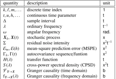
Much of the analysis presented here takes place naturally in the spectral domain. Ordinary frequencies are generally written
as−∞< λ <∞, measured in kHz. In discrete time with
sam-pling interval∆, spectral quantities are periodic inλwith period fs =1/∆, the sampling frequency; we shall sometime restrict
such quantities to the interval−1/(2∆) ≤ λ < 1/(2∆), where
1/(2∆) = fs/2 is theNyqvist frequency. For continuous-time
sequences, spectral quantities are not generally periodic. For discrete-time spectral quantities, it is sometimes convenient to work instead with theangular frequencyω ≡ 2π∆λ. We may
then consider spectral quantities as defined on the unit circle |z| = 1 in the complex planeC, withz = e−iω,
−π ≤ ω < π.
In continuous time we occasionally use a normalised frequency
ω≡2πλ, and spectral quantities may be considered defined on
the imaginary lineRe(ζ)=0 in the complex plane, withζ =iω,
−∞< ω <∞. In the time domain,zandζ may be interpreted
aslag (backshift) operatorsin discrete and continuous time
re-spectively.
The link between time and frequency domains is theFourier transform. Here, Fourier transforms are always defined in terms
of ordinary frequencyλand indicated with a hat symbol over
over the corresponding sequence specifier; e.g. ˆx(λ), or just ˆx
when the entire transform is referenced. In light of the prolif-eration of conventions, our definitions for Fourier transforms are set out inAppendix A; discrete-time transforms are scaled by the sample time step∆in order to ensure that dimensions
are always the same in discrete and continuous time, and that, in particular, limiting values for ∆-subsampled
continuous-time sequences tend to corresponding continuous-continuous-time values as ∆ → 0; see Appendix Afor details. Generally, we take
care to scale by sampling interval so that (almost) all measur-able quantities (Tmeasur-able1) have the same dimensions in discrete and continuous time, and comparisons of magnitudes are thus meaningful, in particular in the limit ∆ → 0. Although this
convention may appear cumbersome, particularly in our analy-sis of discrete-time processes (Section2), the payoffis a more
harmonious and intuitive tie-in with the continuous-time case and subsampling analysis (Section3).
Throughout, superscript “⊺” denotes matrix transpose, super-script “∗” matrix conjugate transpose and| · |the determinant of
a square matrix. A dot over a symbol denotes differentiation
with respect to a continuous time parameter.
2. Discrete VAR processes and Granger Causality
We briefly outline the VAR theory that we shall require; the reader is referred to standard texts (Hamilton,1994;L¨utkepohl,
2005) for details. LetX≡ {Xk|k∈Z}be a discrete-time, purely nondeterministic, zero-mean, wide-sense stationary vector pro-cess. With a view to Granger-causal analysis, we assume the same conditions on the process X as inGeweke (1982). By Wold’s Theorem (Wold,1938;L¨utkepohl,2005)Xhas avector
quantity description unit
k, ℓ,m, . . . discrete time index 1
t,u,h, . . . continuous time parameter t
∆ sample interval t
λ ordinary frequency t−1
ω angular frequency rad.
Xk,X(t) stochastic process x
Σ residual noise intensity x2t−1
Em,E(h) mean-square prediction error (MSPE) x2 Γk,Γ(t) autocovariance sequence/funtion x2
H(λ) transfer function t
S(λ) cross-power spectral density (CPSD) x2t
FY→X Granger causality (time domain) b
fY→X(λ) Granger causality (frequency domain) b Table 1: Notation and dimensions:tdenotes units of time (e.g., ms, so thatt−1is measured in kHz),xdenotes the units of the neural signal under consideration (e.g., volts, tesla, etc.) andbdenotes the unit of information (bits or nats, depending on whether base 2 or natural logarithms are used).
moving-average(VMA) representation
Xk= ∞
X ℓ=0
Bℓεk−ℓ (1)
with square-summable coefficient matricesBℓ(B0=I), andεa white-noise process. Consideringzas thelag operator z·Xk=
Xk−1, we can write (1) in compact form as
Xk= Ψ(z)·εk (2)
where the MA operator
Ψ(z)≡ ∞
X ℓ=0
Bℓzℓ (3)
has the minimum-phase property that|Ψ(z)|,0 for complexz
on the unit disc|z| ≤1. We shall require that the VMA
repre-sentation (1) may be inverted to yield avector autoregressive
(VAR) representation Xk= ∞ X ℓ=1 AℓXk−ℓ+εk (4)
with square-summable coefficient matricesAℓ.Geweke(1982) supplies a condition on the spectrum ofX(see below)—that it is bounded away from zero almost everywhere—which suffices
for invertibility of the VMA representation (Rozanov,1967). The condition (see Geweke,1982, eq. 2.4), which we assume here, also guarantees that any vectorsubprocess ofXhas a VAR representation. We may write the VAR (4) as
Φ(z)·Xk=εk (5) with Φ(z)≡I− ∞ X ℓ=1 Aℓzℓ (6)
Stability of the process requires that|Φ(z)|,0 on|z| ≤1, and
we haveΦ(z)= Ψ(z)−1on|z| ≤ 1. Henceforth, by “VAR
pro-cess” we mean a process satisfying all of the above conditions. In accordance with the conventions described in the Intro-duction, we assume a sample time step∆is always given, and
parametrise the magnitude of the residual noiseεby itsintensity
Σ≡∆−1cov(εk). This is consistent with the additivity of
vari-ance, and ensures that the dimensions ofΣare consistent with
the corresponding quantity in the continuous-time processes we shall encounter later (Section3).
Theautocovariance sequenceΓ≡ {Γk|k∈Z}is given by
Γk≡cov(Xk+ℓ,Xℓ) (7) (by stationarity, this does not depend onℓ) and satisfiesΓ−k = Γk⊺, and theYule-Walker equations
Γk= ∞
X ℓ=1
AℓΓk−ℓ+δk0∆Σ k≥0 (8)
In terms of the VMA coefficients, it is straightforward to show
that Γk= ∆ ∞ X ℓ=0 Bk+ℓΣBℓ⊺ k≥0 (9)
Thecross-power spectral density(CPSD)S forXis defined
for−∞< λ <∞by S(λ)≡ lim K→∞ 1 2K∆cov bXK(λ) (10)
where bXK(λ) ≡ ∆PkK=−KXke−2πi∆λk is the truncated Fourier
transform of the process X. The S(λ) are Hermitian
matri-ces and theWiener-Khintchine Theorem(Wiener,1930; Khint-chine,1934) states that:
S(λ)=bΓ(λ) (11)
at all frequencies; i.e. the CPSD is the Fourier transform of the autocovariance sequence.
The transfer functionfor the VAR (4) is defined to be the
Fourier transform of the MA coefficients:
H(λ)≡bB(λ)= ∆Ψe−2πi∆λ= ∆ ∞
X ℓ=0
Bℓe−2πi∆λℓ (12)
which may also be written as
H(λ)= ∆Φe−2πi∆λℓ−1= ∆ I− ∞ X ℓ=1 Aℓe−2πi∆λℓ −1 (13)
We then have thespectral factorisationformula (Masani,1966)
S(λ)=H(λ)ΣH(λ)* (14)
which holds for all λ. A classical result states that, given a
CPSD S(λ) satisfying certain regularity conditions (Masani, 1966;Wilson,1972), there exists a uniqueΨ(z) holomorphic
symmetric matrixΣ, such that settingH(λ)= ∆Ψ e−2iπ∆λ, (14)
is satisfied. In other words, for a class of CPSDs the spec-tral factorisation (14) isuniquely solvableforH(λ) andΣ, and
hence parameters for a VAR model with the given CPSD may be obtained. Although this result is not constructive—there is no known algorithm for analytic factorisation of an arbitrary CPSD—in specific cases, in particular forrationalspectral
den-sities (Kuˇcera,1991)], it is frequently feasible; see Section4.2
andAppendix Jfor a concrete, nontrivial example.
A VAR of the form (4) is equivalently specified by the VAR parameters (A,Σ), the autocovariance sequenceΓor the CPSD S. The Yule-Walker equations (8), Wiener-Khintchine
Theo-rem (11) and spectral factorisation formula (14) establish recip-rocal relationships between the respective representations. Bar-nett and Seth(2014) exploit these relationships to design effi
-cient computational pathways for the numerical computation of Granger causalities (Section 2.1below). Analytically, we are also free to choose the representation appropriate to the task at hand.
2.1. Granger Causality
Granger causality is most commonly framed in terms of
prediction. Usually, only 1-step-ahead prediction is
consid-ered. Here, for reasons that will become clear (Section 3.3), we consider Granger causality at arbitrary prediction horizons (L¨utkepohl,1993;Dufour and Renault,1998). The optimal (in the least-squares sense)m-step-ahead prediction (m=1,2,. . . )
of the stable VAR (4) based on all information contained in its own (infinite) past—i.e., the optimal prediction of Xk+mgiven the historyX−
k ≡ {. . . ,Xk−2,Xk−1,Xk}of the process up to and
including the kth step—is given by the orthogonal projection EhXk+m|X−kiof Xk+monto X−k. A standard result (Hamilton,
1994) states that EhXk+m| X− k i = ∞ X ℓ=m Bℓεk+m−ℓ (15)
It follows that themean-square prediction error(MSPE) at a
prediction horizon of timem∆into the future, is given by
Em≡cov EhXk+m| Xk−i−Xk+m= ∆ m−1 X ℓ=0 BℓΣBℓ⊺ (16)
In particular,E1is just the residual noise covariance∆Σ, while
from (9),Em → Γ0 as m → ∞; it also makes sense to define
E0≡0, as prediction at zero horizon is exact.
Our exposition of Granger causality follows in spirit the stan-dard formulation of Geweke (1982). Suppose that we have two jointly distributed discrete-time vector stochastic processes (“variables”)X,Yso that the joint process [X⊺Y⊺]⊺is a VAR of the form (4). By assumption, the subprocessesXandYalso have VAR representations. We may then, for a given predic-tion horizonm∆(m=1,2, . . .), compare the MSPEEm,xxof the
predictionEhXk+m| X−
k,Y−k
i
ofXk+mbased on thejointhistory
of XandY(the “full regression”), with the MSPEE′
m,xxof the
predictionEhXk+m| X−kiofXk+mbased only on theself-history
of the subprocessX (the “reduced regression”3). If inclusion of the historyY−
k improves the prediction ofXk+m, then we say
thatY (the “source” variable)Granger-causesX(the “target” variable) at prediction horizonm∆. Geweke (1982) proposed
that prediction be quantified bygeneralised variance4 (Wilks, 1932)—that is, the determinant of the MSPE—leading to the definition FY→X,m≡log E′m,xx Em,xx (17) FX→Y,mis defined symmetrically.
Ifm=1 (1-step prediction), we drop themsubscript. Note
thatE1,xx = ∆Σxx, whereΣxxis thexxcomponent of the noise
intensityΣof the joint process, whileE′1,xx= ∆Σ′xxwhereΣ′xxis
the noise intensity of the subprocessX, considered as a VAR. Thus we obtain the standard 1-step Geweke measure
FY→X≡ FY→X,1=log
Σ′xx
|Σxx|
(18)
FY→X,m ≥ 0 always, since inclusion of the history Y−k in
the full regression can only decrease the prediction error. It may be shown, furthermore (Sims,1972; Caines, 1976), that FY→X =0 iff Ψxy(z)≡0. But from (2) it follows thatΨxy(z)≡ 0 =⇒ Ψ′xx(z)= Ψxx(z), and, since all theBℓare lower block-triangular, from (16) we haveE′
m,xx=Em,xxfor anym. Thus we
may state:
FY→X=0 ⇐⇒ Ψxy(z)≡0 ⇐⇒ FY→X,m=0∀m>0
(19) That is,vanishing1-step GC implies vanishing GC atany pre-diction horizon. The converse does not hold, though:FY→X,m
may vanish form>1 even ifFY→X >0 (cf.Appendix C). In general,FY→X,mwill depend on the prediction horizon. Since
bothEm,xx andE′m,xx → Γ0,xx as m → ∞, FY→X,m → 0 as m → ∞, so that FY→X,m attains a maximum at some finite
value(s) ofm.
At this point we note, as alluded to in the Introduction (Section 1), that Granger causality has a clear information-theoretic interpretation: Barnett et al. (2009) show that for Gaussian processes, Granger causality is entirely equivalent to the non-parametric information-theoretic transfer entropy
measure (Schreiber,2000;Paluˇs et al.,2001), and for general Markovian processes (under a mild ergodicity assumption) the log-likelihood ratio statistic for the Markov model [cf. (D.3)]
converges in the large-sample limit to the corresponding trans-fer entropy (Barnett and Bossomaier, 2013). TE, as a con-ditional mutual information—and by extension GC—is natu-rally measured in units of bits (or nats, if natural logarithms are used).
Regarding Granger’s other requirement for causal effect, that
the information that Y contains about (the future of) X be
3We generally indicate quantities associated with the reduced, as opposed
to full regression, with a prime.
4For a discussion on the preferability of the generalised variance|Σ|over
thetotal variancetrace [Σ], seeBarrett et al.(2010); see also the maximum
unique, here we note just that the effect on Granger causalities
of other (accessible) variables jointly distributed with X and Ymay be discounted by including them in both the full and re-duced predictor sets5. This leads to the definition ofconditional Granger causality (Geweke,1984). While all Granger causali-ties discussed in this paper have conditional counterparts, here we restrict our attention to the unconditional case.
Geweke(1982) refers to the Granger causalityFY→Xas the “linear feedback” fromYtoX, and goes on to define the “in-stantaneous feedback” orinstantaneous causality:
FX·Y ≡log
|Σxx|Σyy
|Σ| (20)
which vanishes iff the residuals εx,k,εy,k are
contemporane-ously uncorrelated.Solo(2007) distinguishes “strong” Granger causality from the conventional (“weak”) variety, noting that only (the existence of) strong causality is strictly preserved un-der subsampling. In a VAR framework, strong causality from Y → X replaces the full (1-step) predictor set X−
k,Y−k with
the predictor set X−
k,Y−k+1 [cf. Geweke (1982, eq. 2.9)]; that is, the contemporaneous source term Yk+1 is included in the full predictor set (the reduced predictor set remains unaltered). The residual errors of the strong least-squares prediction are εx,k−ΣxyΣ−yy1εy,k(Geweke,1982), so that the MSPE is∆×the partialresidual noise intensity matrix
Σxx|y≡Σxx−ΣxyΣ−yy1Σyx (21)
This leads to the statistic
FYstrong→X ≡log Σ′ xx Σxx|y =FY→X+FX·Y (22)
(the last equality follows from block-decomposition of the de-terminant |Σ|). Strong GC, while invariant under subsampling
is, however, unsatisfactory as adirectionalmeasure, since it is
not generally possible to disentangle the directional and instan-taneous contributions.
Although not the focus of this paper, a significant feature of Granger-causal analysis is that (time domain) GC may be decomposed in a natural way by frequency. The resulting frequency-domain, or spectralGranger causality integrates to
the time-domain GC (18). For a full derivation and discussion we refer toGeweke(1982); here we just present the definition of the spectral GC fromYtoX:
fY→X(λ)≡log |
Sxx(λ)|
Sxx(λ)−Hxy(λ)Σyy|xHxy(λ)∗
(23)
whereΣyy|x≡Σyy−ΣyxΣ−xx1Σxy[cf.(21)]. fY→X(λ) is always non-negative, and Geweke’s fundamental spectral decomposition of
5Of course this is only possible foraccessiblevariables - inaccessible
(hid-den, latent) influences are in general problematic for causal analysis in a broader sense (Valdes-Sosa et al.,2011).
Granger causality applies6
FY→X= ∆ Z 1
2∆
−21∆
fY→X(λ)dλ (24)
The spectral GC (23) is, at any specific frequency λ, also
a quantity of information measured in bits or nats, and (24) presents time-domain GC as an average over all frequencies of spectral GC. We remark that a spectral counterpart forFX·Yhas been defined (Ding et al.,2006), but is somewhat unsatisfactory insofar as it may become negative at some frequencies and lacks a compelling physical interpretation.
It is known (Geweke, 1982;Barnett and Seth, 2011;Solo,
2016) that 1-step Granger causality, in both time and frequency domains, is invariant under (almost) arbitrary causal, invertible (stable, minimum-phase7) filtering; seeAppendix Bfor more detail. However, as demonstrated inAppendix C, invariance doesnotextend tom-step GC form > 1, unlessΨxy(z) ≡0
-equivalently,FY→X =0. In that case filter-invariance does hold for m ≥ 1; that is, causal, invertible filtering will not induce spuriousGranger causalities at any prediction horizon.
VAR modelling is particularly suited to data-driven ap-proaches to functional analysis (Appendix D) and its applica-bility quite general. By the Wold decomposition theorem ( Han-nan,1970), any covariance-stationary stochastic process in dis-crete time has a moving-average (MA) representation. Further spectral conditions may be imposed so that the Wold MA repre-sentation may be inverted to yield a stable VAR reprerepre-sentation (4) (Rozanov,1967). We assume that these conditions apply for all discrete stochastic processes encountered in this study. We note that if there is nonlinear (delayed) feedback in the gener-ative process, while this does not preclude VAR-based estima-tion of Granger causalities (provided the VAR representaestima-tion criteria mentioned above hold), a linear model will not be par-simonious and transfer entropy (or a suitable nonlinear model-based version of Granger causality) may be preferable ( Bar-nett and Bossomaier,2013). In general, though, VAR-based Granger causality has the advantages of simplicity, ease of es-timation, a known sampling distribution and a natural spectral decomposition.
More recently, a theory of Granger causality has been devel-oped forstate-spaceprocesses (Barnett and Seth,2015;Solo, 2016). The state-space approach offers some significant
advan-tages from modelling, estimation and computational perspec-tives. This, as well as estimation, statistical inference and de-tection of (discrete-time) Granger causality from empirical time series data, is discussed inAppendix D.
6Strictly speaking, equality in (24) holds provided the condition
Ayy(z)−ΣyxΣ−xx1Axy(z),0 is satisfied for allzon the unit disc|z| ≤1;
oth-erwise it should be replaced by≤. In practice, according toGeweke(1982), the equality condition is “almost always” satisfied.
7Minimum phase requires that the inverse filter also be stable; note that in Barnett and Seth(2011) this requirement is erroneously overlooked [thanks to Victor Solo (personal communication) for bringing this to our attention].
3. Distributed-lag vector autoregressive processes in con-tinuous time
Following the discussion in Section 1regarding the essen-tially continuous-time nature of biophysiological processes, in order to address the impact of subsampling we require appro-priate continuous-time generative processes for which Granger causality may be defined. Accordingly, we start with an un-derlying analogue neurophysiological process U(t) in contin-uous time8 t and an observation function ξ(·). The observed (multivariate) signal X(t) = ξ(U(t)) is then sampled at
regu-lar discrete time intervals. U(t) may be stochastic (endogenous
noise), as may be the observation function (exogneous, mea-surement noise), so that X(t) is considered a continuous-time
stochastic process. Our approach is to assume thatX(t) admits
a continuous-time linear autoregressive representation. The standard multivariate linear autoregressive model in con-tinuous time is the vector Ornstein-Uhlenbeck (VOU) process (Uhlenbeck and Ornstein,1930;Doob,1953) defined by a lin-ear stochastic differential equation (SDE)
dX(t)=AX(t)dt+dW(t) (25)
whereW(t) is a vector Wiener process. The process (25) must,
however, be considered implausible as a model for an observed neurophysiological processes, since it fails to model delayed feedback atfinitetime scales. To address this we generalise the
VOU process to the CTVAR (continuous-time vector autore-gressive) process described below.
Our construction closely mirrors that of the discrete-time VAR case (Section 2). Thus we assume that the continuous-time, wide-sense stationary, stable, minimum-phase (and zero-mean) vector process X ≡ {X(t)|t ∈ R} admits a moving-average representation (Caines and Chan,1975;Comte and Re-nault,1996)
X(t)=
Z ∞
u=0
B(u)dW(t−u) (26)
whereW(t) is again a vector Wiener process9, the MA kernel B(u) [with B(0) = I] is square-integrable and the integral is
to be interpreted as an It¯o integral(Øksendal,2003). In
con-tinuous time we define the lag operatorζ as follows: suppose
that a complex-valued functionL(ζ) may be written (uniquely)
as a Laplace transform L(ζ) = R0∞L(u)e−ζudu. Then for a
continuous-time processU(t), we define L(ζ)·U(t) as the It¯o
integralRu∞=0L(u)dU(t−u), and (26) may be written as
X(t)= Ψ(ζ)·W(t) (27) where Ψ(ζ)≡ Z ∞ 0 B(u)e−ζudu (28)
The minimum-phase property requires that|Ψ(ζ)| , 0 on the
right half-planeRe(ζ)≥0.
8The unit of time is taken to be the same as for discrete-time processes. 9This might be generalised to continuous-time white noise processes as
de-fined for the continuous-time Wold decomposition theorem (Rozanov,1967).
As in the discrete-time case, we assume that the MA repre-sentation (26) may be inverted to yield a continuous-time vector autoregressive (CTVAR) representation as a stochastic linear integro-differential equation (Comte and Renault,1996)
dX(t)= Z ∞ 0 A(u)X(t−u)du dt+dW(t) (29) or Φ(ζ)·X(t)=W(t) (30) with Φ(ζ)≡ζI− Z ∞ 0 A(u)e −ζu du (31)
To verify (30,31), note thatΦ(ζ) may be written as the Laplace
transform of ˙δ(u)I−A(u), where ˙δ(u) denotes the derivative, in
the generalised function sense, of the delta functionδ(u); (30)
then follows from the relationR∞
−∞δ˙(u)ϕ(t−u)du=ϕ˙(t) for any
functionϕ(u) (Friedlander and Joshi,1998). Stability requires
that|Φ(ζ)| , 0 on the right half-planeRe(ζ) ≥ 0, and in
Ap-pendix Ewe prove thatΨ(ζ) = Φ(ζ)−1 on the right half-plane
Re(ζ)≥0
The AR kernelA(u) specifies causal, time-lagged coupling
between nodes over a range of feedback delaysu, whiledW(t)
represents continuous-time white noise with (positive-definite) covariance matrixΣdt, so thatΣagain represents residual noise intensity. We assumeA(u) be besquare-integrable10and allow
it to be ageneralised function(Friedlander and Joshi,1998), so
it might, for example, include delta functions. The integral over
uin (29) is then taken to be a Lebesgue integral. Note that the
VOU process (25) is a special case of (29) withA(u)= Aδ(u)
a delta function at “infinitesimal lag”u=0. Analagous to the
discrete-time case, we also assume that any vectorsub-process
ofX(t) may be represented as a CTVAR11.
Stochastic integro-differential equations similar to (29) have
been studiedin abstracto, as models for various physical,
engi-neering and biological phenomena, and (more along the present lines) in the econometrics literature (Sims, 1971; Geweke,
1978;McCrorie and Chambers,2006). They have not however, as far as we are aware, been deployed previously in the neu-rosciences. Our approach most closely resembles the “CIMA” processes presented inComte and Renault(1996); our empha-sis, however, is more on the autoregressive and (as we shall see later)predictiveaspects of the model.
InAppendix Fwe show that the MA kernelB(u) satisfies
˙
B(u)=
Z u
0 A(s)B(u−s)ds u≥0 (32a)
B(0)=I (32b)
where ˙B(u) denotes differentiation from the right12with respect
tot.
10This condition may be unnecessarily restrictive; we require at least that the
CPSD ofX(t) (see below) exists (Lighthill,1958).
11It seems plausible, although we have not established this rigorously, that
this may follow from a similar boundedness condition on the CPSD to that described inGeweke(1982).
12We shall generally assume that appropriate derivatives exist wherever they
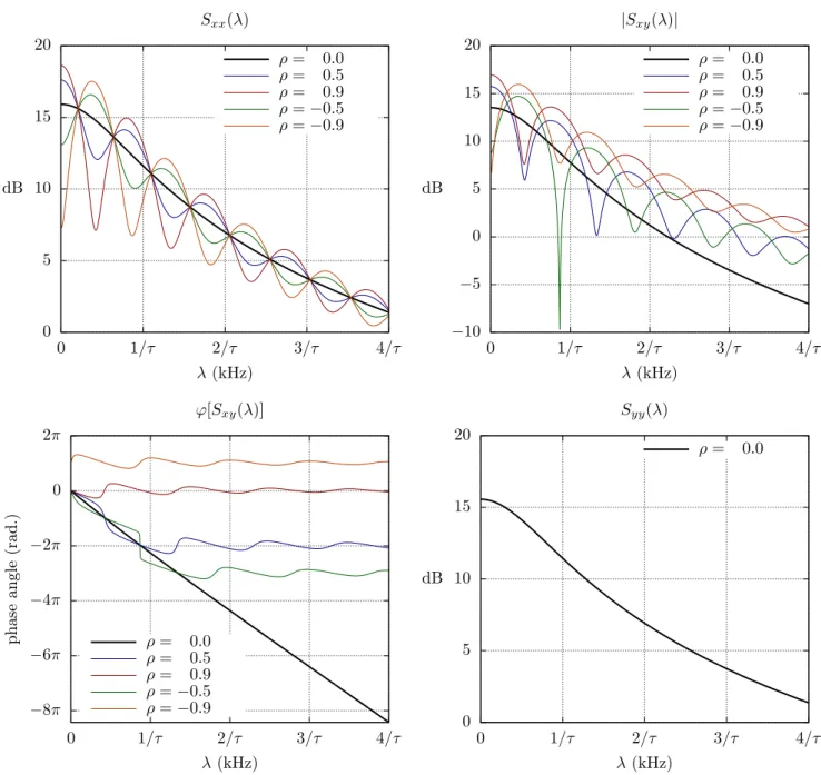
The autocovariance function of a stationary continuous-time vector stochastic process is defined as
Γ(t)≡cov(X(t+u),X(u)) (33)
which again, by stationarity, does not depend onu, andΓ(−t)= Γ(t)⊺. From the MA representation (27) an application of the
It¯o isometry(Øksendal,2003) yields
Γ(t)=
Z ∞
0
B(t+u)ΣB(u)⊺ du t
≥0 (34)
From (34) we may derive the continuous-time Yule-Walker equations for the process (29)
˙ Γ(t)= Z ∞ 0 A(u)Γ(t−u)du t>0 (35a) ˙ Γ(0)+Γ˙(0)⊺= −Σ (35b)
where ˙Γ(t) denotes differentiation from the right.
Analogous to the discrete-time case, the CPSD for the pro-cess is defined by S(λ)≡ lim T→∞ 1 2T cov bXT(λ) (36) on−∞< λ <∞, now withbXT(λ)≡RT −TX(t)e− 2πiλtdt[cf.(10)],
and the Wiener-Kintchine Theorem in continuous time again reads:
S(λ)=bΓ(λ) (37)
The continuous-time transfer function is again defined as
H(λ)≡bB(λ)= Ψ(2πiλ)=
Z ∞
0
B(u)e−2πiλudu (38)
which may also be written as
H(λ)= Φ(2πiλ)−1= 2πiλI− Z ∞ 0 A(u)e−2πiλudu !−1 (39)
and from (34) it is not hard to establish the continuous-time spectral factorisation13
S(λ)=H(λ)ΣH(λ)* (40)
We note thatH(λ) satisfies
lim |λ|→∞2πiλH(λ)=I (41) so that from (40) lim |λ|→∞4π 2λ2S(λ)= Σ (42)
i.e., S(λ) decays as λ−2, as |λ| → ∞. We conjecture
that, analagous to the discrete-time case, given a continuous-time CPSD S(λ) satisfying suitable regularity conditions,
there exists a unique Ψ(ζ) holomorphic on Re(ζ) ≥ 0 with lim|ω|→∞ iωΨ(iω) = I and positive-definiteΣ, such that (40) is satisfied forH(λ)= Ψ(2πiλ) on−∞< λ <∞.
13This follows from the continuous-time versions of the Wiener-Kintchine
and Convolution theorems, noting that (34) may be written asΓ(t)=(B∗B⊺)(t)
whereB(u)≡B(u)L, withLa matrix square root ofΣsatisfyingLL⊺= Σ(by
positive-definiteness, such anLexists).
3.1. Subsampling a CTVAR process
We next examine some properties of the discrete-time pro-cesses X(∆) obtained by subsampling a CTVAR processX at fixed time intervals ∆; i.e., Xk(∆) ≡ X(k∆). It is these ∆
-subsampled processes which stand as models for discretely-sampled neurophysiological recordings of an underlying bio-physiological process (Section1). A subtlety which we must address is that, while a∆-subsampling of a (stable,
minimum-phase) CTVAR is itself always stable, there is no guarantee that it will be minimum-phase for all ∆ - see e.g., Åstr¨om et al.
(1984). We thus assume that the minimum-phase condition for ∆-subsamplings holds as necessary [in worked examples
(cf.Section 4.2) it must be tested explicitly], and that in
par-ticular (cf.Section3.3below) it holds in the limit of fine
sub-sampling; that is, there exists a sampling interval∆0such that
for any∆-subsampling with 0 < ∆ ≤ ∆0, X(∆) is minimum
phase.
With a view to calculation of (multistep) Granger causalities (Section2.1), we require expressions for the transfer function, residual noise intensity, MA coefficients and CPSD of the ∆
-subsampled processes. The crucial observation is that the au-tocovariance sequenceΓ(∆) of the subsampled processX(∆) is
justΓk(∆)= Γ(k∆), whereΓis the autocovariance function of
the original continuous-time process - this follows immediately from (33) and (7). Recall that for calculation of time-domain multistep Granger causalities for a discrete-time process, we require the residual noise intensity matrices and the firstm−1
MA coefficients (wheremis the number of prediction steps) of
the process itself and also of subprocesses (16,17). In the fre-quency domain we need the transfer function, evaluated at the requisite frequencies (12,14,23). Analytically, while in princi-ple the∆-subsampled VAR parameters might be derived from
the autocovariance sequence via the discrete-time Yule-Walker equations (8) (cf.our remarks in Section2regarding the
multi-ple representations for a VAR process), in practice this is gen-erally intractable, and it is more convenient to calculate them from the discrete-time CPSD by spectral factorisation14.
Given a CTVAR specified by an autoregressive coefficients
kernel A(u) and residuals covariance matrix Σ, a procedure
for analytic calculation of multistep Granger causalities for the discrete-time∆-subsampled process is described in Table2. In
Section4.1below we follow precisely this procedure for a non-trivial analytic example.
InAppendix Gwe establish firstly an asymptotic expansion for the CPSD of the subsampled process in the limit∆→0
S(λ;∆)=S(λ)+121∆2Σ +7201 ∆4(Ω +12π2λ2Σ)+O∆5 (43)
where Ω ≡ ...Γ(0) + ...Γ(0)⊺, and also the scaling relations
14Solving forAk,Σfrom (8) involves a matrix deconvolution, which is
gener-ally difficult to perform analytically. In the frequency domain, the Convolution
Theorem—which underlies the spectral factorisation formula (14)—renders the deconvolution more tractable. In continuous time, however, the integro-differential Yule-Walker equations (35) may well be more tractable (cf.
1. Calculate the continuous-time MA kernelBby direct solution
of (32).
2. Calculate the continuous-time autocovariance functionΓas fol-lows: either
(a) Calculate the continuous-time transfer functionH(38).
(b) Calculate the continuous-time CPSDS(40).
(c) CalculateΓby inverse Fourier transform (37). or
(d) CalculateΓby integration (34). or
(e) Calculate Γ by direct solution of the continuous-time Yule-Walker equations (35).
3. Calculate the discrete-time subsampled process autocovariance sequenceΓ(∆) byΓk(∆)= Γ(k∆).
4. Calculate the subsampled process CPSDS(∆) by discrete-time Fourier transform ofΓ(∆) (11).
5. Calculate the subsampled process transfer function H(∆) and residuals intensityΣ(∆) by discrete-time spectral factorisation ofS(∆), for both full and (time-domain only) reduced models (14).
6. Time domain (1-step): calculate Granger causality from full and reduced subsampled residuals intensities (18).
7. Time domain (m-step):
(a) Calculate subsampled MA coefficients Bk(∆) up tok =
m−1 by inverse Fourier transform of the subsampled
transfer functionH(∆), for both full and reduced models (12).
(b) Calculate MSPEsEm(∆) from Σ(∆) and the Bk(∆), for
both full and reduced models (16).
(c) Calculate subsampledm-step Granger causality from the
full and reduced MSPEs (17).
8. Frequency domain: calculate frequency domain Granger causality from (full model)Σ(∆),S(∆) andH(∆) (23).
Table 2: Procedure for analytical calculation of multistep time-domain and/or spectral Granger causalities for a∆-subsampled CTVAR process from known CTVAR
parametersA(u),Σ.
(Zhou et al.,2014)
H(λ;∆)=H(λ)+O(∆) (44a) Σ(∆)= Σ +O(∆), (44b)
while from (9) and (34) we have:
Bk(∆)=B(k∆)+O(∆) (45)
3.2. Subsampling a VOU process
The special case of subsampling a vector Ornstein-Uhlenbeck process, i.e., where A(u) = Aδ(u), may be solved
exactly. The Yule-Walker equation (35a) becomes the ordinary differential equation ˙Γ(t)=AΓ(t), with solution
Γ(t)=eAtΓ(0) t≥0 (46)
and from the initial condition (35b), Γ(0) satisfies the
continuous-time Lyapunov equation
AΓ(0)+ Γ(0)A⊺=
−Σ (47)
The autocovariance sequence for the ∆-subsampled process is
thus
Γk(∆)=e∆AkΓ(0) (48)
Now it is easily calculated from the discrete-time Yule-Walker equations (8) that the discrete-time VAR(1) process Xk = AXk−1+εkhas autocovariance sequenceΓk =AkΓ0, whereΓ0
satisfies the discrete-time Lyapunov equationΓ0−AΓ0A⊺= ∆Σ.
Since a VAR process is uniquely identified by its autocovari-ance sequence, we thus find that the subsampled processX(∆)
is VAR(1) (which underlines the unsuitability of VOU pro-cesses as models for neurophysiological data). The (1-lag) co-efficient matrix and residual noise intensity are given
respec-tively by
A(∆)=e∆A (49a)
Σ(∆)= ∆−1hΓ(0)−e∆AΓ(0)e∆A⊺i (49b)
Note that in general a subprocess of a VOU process willnotbe
VOU, nor will a subsampled subprocess be VAR(1).
3.3. Granger causality for CTVAR processes
It is not immediately clear how we should define Granger
causality for continuous-time processes in general, and for CT-VAR processes (considered as natural continuous-time ana-logues of VAR processes) in particular. As we shall see, if we attempt to calculate Granger causality at an “infinitesimal” pre-diction horizon, then prepre-diction errors becomes negligible and, in particular, full and reduced prediction errors decay to zeroat the same rate(Renault and Szafarz,1991;Comte and Renault, 1996;Renault et al.,1998); thus Granger causality vanishes in the infinitesimal horizon limit. This suggests that we consider prediction atfinitetime horizons; that is, a Granger causality
measureFY→X(h) based on a prediction horizon a finite timeh into the future (Comte and Renault,1996;Florens and Foug`ere,
1996). We would also like continuous-time GC to be, in a pre-cise sense, the limiting case of discrete-time GC under increas-ingly fine subsampling.
We are thus lead to consider optimal prediction of X(t + h) given the history X−(t) ≡ {X(s)|s ≤ t} of the process
X up to and including time t. The orthogonal projection EX(t+h)| X−(t) may be expressed as the limiting case, as
∆ → 0, of the expectation of X(t +h) conditioned on a∆
-subsampling of the historyX−(t):
EX(t+h)|X−(t)=
lim ∆→0E[
X(t+h)| X(t),X(t−∆),X(t−2∆), . . .] (50)
Then, setting ∆ = h/m, this is just the limit as m → ∞ of
the optimal m-step prediction of theh/m-subsampled process
X(h/m)—recall that by assumption (Section3.1) it has a stable,
minimum-phase VAR representation, at least for large enough
m—and from (15) and (45) we obtain in the limit
EX(t+h)| X−(t)=
Z ∞
u=h
B(u)dW(t+h−u) (51)
An application of the It¯o isometry then yields the continuous-time MSPE E(h)≡cov EX(t+h)| X−(t)−X(t+h) = Z h 0 B(u)ΣB(u)⊺du, h ≥0 (52)
Alternatively, we might have defined the continuous-time MSPE at horizonhas the limit of its subsampled counterpart:
E(h)≡ lim
m→∞Em(h/m), h≥0 (53)
where Em(h/m) denotes the m-step MSPE of the h/m
-subsampled process. By (16), (44b) and (45) the definitions coincide. Note that convergence in (53) is from above: for fixed
m≥1 and any integerr >1,Erm(h/rm)≤ Em(h/m), since the
corresponding orthogonal projections predict the process at the same horizon (i.e., timehinto the future), but therm-step
pre-diction is based on a superset of the historic predictor set of the
m-step prediction. SinceEm(h/m)≥0 for anym≥1, the limit
(53) thus exists. From (52)E(h) satisfies the ordinary diff
eren-tial equations ˙
E(h)=B(h)ΣB(h)⊺ h
≥0 (54a)
E(0)=0 (54b)
For a joint CTVAR process [X⊺Y⊺]⊺, we now define Granger causality at horizonhin continuous time analagously
to the discrete-time case (17) as
FY→X(h)≡log|E ′ xx(h)| |Exx(h)| , h≥0 (55) whereE′
xx(h) denotes the continuous-time MSPE at horizonh
for the subprocessX(recall that by assumptionXhas a CTVAR representation). From (17) and (53) we have
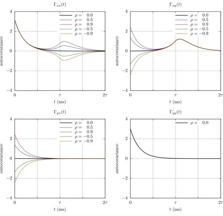
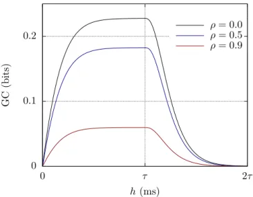
FY→X(h)= lim
m→∞FY(h/m)→X(h/m),m, h≥0 (56)
so that continuous-time GC may be defined as the limit of
discrete-time GC under progressively finer subsampling, whilst holding the prediction horizonhfixed (FIG.1).
Clearly FY→X(h) ≥ 0 always. We now show that FY→X(h)→0 linearly ash→0 [cf.Zhou et al.(2014)]. From (54) we haveE(0)=0 and ˙E(0)= Σ, so that from (55)
FY→X(h)=log hΣ′ xx+O h2 hΣxx+Oh2 (57)
ash→0. Now the CPSD ofXmay be written in two ways as
Sxx(λ)=H(λ)ΣH(λ)∗xx=H′xx(λ)Σxx′ H′xx(λ)∗ (58)
whereH′
xx(λ),Σ′xxdenote respectively the transfer function and
residual noise intensity associated with the reduced CTVAR. Multiplying through byλ2 and lettingλ → ∞, from (41) we
obtainΣ′
xx = Σxxand by (57) we see that [as noted byRenault and Szafarz(1991);Florens and Foug`ere(1996) andComte and Renault(1996)],FY→X(h)→0 ash→0.
Intuitively, this result may be thought of as follows: in-sofar as the transfer function H(λ) represents the input →
output response of the system, (41) indicates that on short timescales (λ→ ∞), the off-diagonal elements ofH(λ)
(cross-response) decay to zero faster than the on-diagonal elements (self-response). Thus at short predictive time scales, condi-tional on their past joint history, the variablesX,Yeffectively
decouple.
From (52) and (34), se see that both Exx(h) andE′xx(h) → Γxx(0) ash→ ∞, so thatFY→X(h)→0 ash→ ∞. Thus, unless identically zero,FY→X(h) will attain a maximum at some finite horizon 0<h<∞.
In contrast toFY→X(0), thezero-horizon Granger causality
rate15 RY→X ≡lim h→0 1 hFY→X(h)=∆lim→0 1 ∆FY(∆)→X(∆) (59)
[the last equality follows from (57) and (44b)] will generally be non-zero. Setting
D≡ 12E¨(0)= 12B˙(0)Σ + ΣB˙(0)⊺ (60)
[the last equality follows from differentiating (54a)], from (59)
and (55) and noting thatRY→X=F˙Y→X(0), we have16
RY→X=trace h
Σ−xx1 D′xx−Dxxi (61)
whereD′
xxdenotes the corresponding quantity for the reduced
CTVAR.RY→Xmay be considered an information transfer rate, measured in bits or nats per unit time.
While (as for the discrete-time, multistep case) we do not have a workable definition for spectral GC fY→X(λ;h) at finite
15The Granger-causal concept underlying this quantity has been described
in the econometrics literature as “local causality” or “instantaneous causality”. Here we do not use the former term, since “local” is more commonly associated withspatialrather thantemporalproximity, nor the latter, to avoid confusion
with whatGeweke(1982) terms “instantaneous feedback”, an entirely distinct concept.
16This follows from the standard formula for the derivative of the
log-determinant of a square matrix function: d
dtlog|M(t)|=trace
h
t t−h/m t−2h/m t−3h/m time predict t+h=t+m(h/m)
FIG. 1: Illustration of prediction underlying eq. (56):FY→X(h) is the limit of the subsampled discrete-timem-step GCFY(h/m)→X(h/m),mat fixed prediction horizon h =m(h/m) under progressively finer subsampling (m→ ∞). Note that the historic predictor set{X(s),Y(s)|s=t,t−h/m,t−2h/m,t−3h/m, . . .}becomes progressively more detailed asmincreases, approaching the continuous-time predictor set{X(s),Y(s)|s≤t}asm→ ∞.
prediction horizonh, we define at least the zero-horizon spectral
GC in continuous time (again measured in bits or nats) as
fY→X(λ; 0)≡log |
Sxx(λ)|
Sxx(λ)−Hxy(λ)Σyy|xHxy(λ)∗
(62)
In contrast to the time-domain GC, spectral GC does not gener-ally vanish at zero prediction horizon; for anyλ, the pointwise
limit as ∆ → 0 of the∆-subsampled spectral GC is equal to
fY→X(λ; 0):
lim
∆→0fY(∆)→X(∆)(λ)=fY→X(λ; 0) (63)
This follows from the discrete-time spectral GC definition (23) via (43), (44a) and (44b). From (24) we then obtain a spectral decomposition for the continuous-time zero-horizon GC rate:
RY→X= Z ∞
−∞
fY→X(λ; 0)dλ (64)
It is not quite obvious thatΨxy(ζ)≡0 =⇒ FY→X(h)=0 for allh>0. This may be seen as follows:Ψxy(ζ)≡0 implies that
the MA kernelB(u) and transfer functionH(λ) are lower
block-triangular. From (40) it follows that the CPSD ofXis given by
Sxx(λ)=[H(λ)ΣH(λ)∗]xx=Hxx(λ)ΣxxHxx(λ)∗, so that [cf.(58)] Σ′xx= Σxxand, since the MA kernel is the inverse Fourier
trans-form of the transfer function,B′xx(u) =Bxx(u). From (52) and
(55) it then follows thatFY→X(h)=0 for anyh, and thence that RY→X =0. By a result ofComte and Renault(1996, Prop. 17) the converse also holds; that is,RY→X=0 =⇒ Ψxy(ζ)≡0, so that we may state17
RY→X=0 ⇐⇒ Ψxy(ζ)≡0 ⇐⇒ FY→X(h)=0∀h>0 (65) This result may be considered a continuous-time analogue of (19). In contrast to the discrete-time case, where it is possible thatFY→X >0 butFY→X,m =0 for somem>1 (Section2.1
andAppendix C), it is not clear whether we may haveRY→X >
17R
Y→X =0 is equivalent to whatComte and Renault(1996) describe as “local noncausality”, whileFY→X(h)=0∀h>0 corresponds to “global non-causality”. The former is shown to be equivalent toΦxy(ζ)≡0; in the uncon-ditionalGC case considered here, this is equivalent toΨxy(ζ)≡0. We note
also thatCaines and Chan(1975), regarding some results which would seem to support this result (at least for rational transfer functions), remark that: “[. . . ] the definitions and results in this paper are also applicable to continuous time processes”, where by “continuous time processes” they refer explicitly to pro-cesses of the form (26).
0 but FY→X(h) = 0 for someh > 0 (we have not found any examples of such behaviour, either analytically or numerically). In general, there is no reason to suppose thatFY→X(h) ≡0 will imply the vanishing ofFY(∆)→X(∆) for a∆-subsampling; that is (Comte and Renault, 1996), subsampling a CTVAR may induce spurious Granger causality. We remark that it is
non-trivial to verify this phenomenon analytically by example (cf.Section4below). Indeed, it is not hard to see that spurious
causality cannot occur for a subsampled VOU process (Comte and Renault,1996, Prop. 21). In this case (Section 3.2), we haveΨxy(ζ)≡0 ⇐⇒ Axy =0, where the VOU AR kernel is A(u) =Aδ(u), and (49a) implies immediately that Axy(∆) =0
where A(∆) is the VAR(1) AR coefficient matrix for the ∆
-subsampled process, so thatFY(∆)→X(∆)=0 for any∆.
Further-more, the analysis of higher-order SDEs inComte and Renault
(1996, Sec. 3) would appear to imply that for a 2×1-dim (bivari-ate) CTVAR, spurious causality cannot arise (cf.Section4.2).
In general, it is possible thatFY(∆)→X(∆) >FY→X(∆) for some ∆values (cf.Section4.2, FIG.8).
Our discussion (Section 2.1) regarding filter-invariance of GC in discrete time suggests that, for h > 0, FY→X(h) will not in general be invariant under a continuous-time causal in-vertible filterG(ζ) =R0∞G(u)e−ζuduwith lim|ω|→∞G(iω)= I andGxy(ζ)≡0; this is indeed the case - see Section4.1below
for an example. As in the discrete-time case, filter-invariance does hold ifΨxy(z)≡0, so that again causal, invertible filtering
will not induce spurious causality at any prediction horizon. It may also be confirmed that filter invariance always holds at zero prediction horizon18; that is,
RY→Xand fY→X(λ; 0) are invariant under causal, invertible filtering.
3.4. Estimation and inference of Granger causalities for sub-sampled continuous-time data
In an empirical setting, given neural data in the form of a discrete subsampling of an underlying continuous-time neuro-physiological process, our standpoint is that the objective of GC-based functional analysis is to estimate as best we can (and perform statistical inference about) Granger causalities
for the underlying neurophysiological process. That is,
hav-ing access only to a∆-subsampling of a joint continuous-time
process [X⊺Y⊺]⊺, our aim is to estimate as well as possible
18The argument ofAppendix Bgoes through verbatim for f
Y→X(λ; 0); then (64) establishes invariance forRY→X. Alternatively, we may take the limiting case∆→0 in (59) under a suitable discretisation ofG(ζ).