Computing multiple-output regression quantile regions

Computing Multiple-Output Regression Quantile Regions

Davy Paindaveinea,∗, Miroslav ˇSimanb

a_{E.C.A.R.E.S. and D´epartement de Math´ematique, Universit´e Libre de Bruxelles, Av.} F.D. Roosevelt, 50, CP114, B-1050 Brussels, Belgium, Tel: +3226503845, Fax: +3226504475 b_{Institute of Information Theory and Automation of the ASCR, Pod Vod´arenskou vˇeˇz´ı 4,}

CZ-18208, Prague 8, Czech Republic

Abstract

Hallin, Paindaveine and ˇSiman (2010) introduced a new concept ofdirectional

regression quantiles extending to the multiple-output setup the traditional Koenker and Bassett regression quantiles. When considering all directions, these new quantiles generate regression quantile regions that, when the only regressor is the intercept, happen to coincide with the classical halfspace depth regions. These quantile regions are powerful data-analytical tools, but their computation is a very challenging problem. The present paper elegantly solves this problem by means of linear programming techniques. We describe in detail the algorithm solving the parametric programming problem involved, and illustrate the resulting procedure on simulated and real data. We also evaluate the efficiency of our Matlabimplementation of

∗_{Corresponding author.}

Email addresses: [email protected](Davy Paindaveine),[email protected] (Miroslav ˇSiman)

the algorithm through extensive simulations. To the best of our knowledge, our code is the first one that allows for computing halfspace depth regions beyond dimension two.

Keywords: Halfspace depth, multiple-output regression, parametric linear programming, quantile regression

2000 MSC: 65C60, 62J99

1. Introduction

Applications of Koenker and Bassett (Econometrica 1978)’s celebrated theory of quantile regression are without number, virtually in all quantitative fields, including economics and econometrics, biomedical studies and clinical trials, biostatistics, and environmental studies; see Koenker (2005) for an extensive presentation of the topic. Quantile regression techniques have been quickly extended to nonlinear and nonparametric regression, and modified for handling count, longitudinal, time series or censored data. Due to the lack of a satisfactory concept of multivariate quantile, however, these techniques have for long been restricted to single-output regression problems, which constitutes a severe limitation.

Various works tried to extend quantile regression to the multiple-output context; see, e.g., Chaudhuri (1996), Koltchinskii (1997), Chakraborty (2003), Wei (2008), or Kong and Mizera (2008). Here, we focus on the recent con-tribution of Hallin, Paindaveine and ˇSiman (2010), hereafter referred to as HPˇS10, which introduces multiple-output regression quantiles based on a directional version of the traditional (single-output) Koenker and Bassett re-gression quantiles. Through the rere-gression quantile regions they generate,

these new quantiles bring to the multiple-output regression context a pow-erful data-analytical tool. In the location case, the corresponding regions happen to coincide with the Tukey (1975) halfspace depth regions. The ob-jective of this paper is to develop a comprehensive and efficient solution to the crucial problem of computing the aforementioned (regression) quantile regions.

We start by quickly describing the regression quantiles introduced in HPˇS10. Consider a multiple-output problem where the m-variate response Y is to be regressed on the p-variate vector of regressors X = (1,W0)0, so that

{(w0,y0)0 : w ∈ _Rp−1_{,y ∈}

Rm} = Rp−1 × Rm is the natural space for considering fitted regression “objects”. Assume that we are given corre-sponding data points (xi,yi) ∈ Rp ×Rm, i = 1, . . . , n, and fix τ ∈ (0,1)

and u ∈ Sm−1 _{:= {y ∈}

Rm : kyk = 1}. In this empirical setup, the HPˇS10 regression (τu)-quantile of they_i’s with respect to the xi’s is defined as any

element of the collection Π(τnu) of hyperplanesπ(τnu):={(w0,y0)0 ∈Rp−1×Rm :

b b0_τuy−a_b0_τu(1,w0)0 = 0}, with (_ba0_τu,bb 0 τu) 0 _∈ arg min n X i=1 ρτ(eb 0 y_i−a_e0xi) subject to u0eb= 1, (1)

where ρτ(x) = x(τ −I(x < 0)) is the well-known τ-quantile check

func-tion. In other words, this regression (τu)-quantile simply is the traditional (single-output) Koenker and Basset regression quantile of order τ obtained when considering, in the m+p−1 Euclidean space, the oriented vectorial line bearing u as the “vertical” axis (that is, as the axis of the univariate response). In the single-output case m = 1, the regression (τu)-quantiles, for u = 1 and u = −1, reduce to the usual regression quantiles of order τ

and 1−τ, respectively.

Now, each optimal solution (a_b0_τu,bb 0

τu)0 to (1) can be associated with the

upper (τu)-quantile halfspace Hτ(nu)+ = {(w0,y0)0 ∈ Rp−1 × Rm : bb 0

τuy −

b

a0_τu(1,w0)0 ≥ 0}. For any τ ∈ (0,1), the sample τ-quantile region is then defined as R(n)(τ) := \ u∈Sm−1 \ H_τ(n_u)+ , (2) where T

Hτ(nu)+ stands for the intersection over all optimal solutions

cor-responding to fixed τ and u. In the location case p = 1, these regions were shown to coincide with the Tukey (1975) halfspace depth regions; see Theo-rem 4.2 of HPˇS10. In the general regression case p > 1, they form a family of nested polyhedral regions wrapping, up to the classical quantile cross-ings, a median or deepest regression hypertube. Hence, beyond extending the single-output Koenker and Bassett regression quantiles to the multiple-output context, this construction also leads to a concept of multiple-multiple-output regression halfspace depth (note that this depth concept, however, has the nature of a point regression depth, hence is distinct from the Rousseeuw and Hubert (1999) regression depth concept, which is a hyperplane depth con-cept). Most importantly, the quantile regions in (2) allow for a much richer regression analysis than any traditional multiple-output regression method can provide; see Section 7 of HPˇS10 for an illustration.

Computing these quantile regions, however, is a very challenging problem even when all the regression (τu)-quantiles are uniquely defined. Then each such regression quantile hyperplane (as any standard single-output Koenker and Basset regression quantile hyperplane in_Rm+p−1_{) must containm+p−1}

abso-lutely continuous with respect to the Lebesgue measure. This implies that the collection of all such regression quantiles is finite, and that the corresponding quantile regions could then be in principle computed exactly. Nevertheless, considering all (m+p−1)-tuples of data points is unfeasible for practical data sets, and so the problem of computing the quantile regions remains a very difficult one. It should be noted that this problem is delicate even in the location case, where the quantile regions coincide with the halfspace depth regions, the computation of which is notoriously difficult. Although there are some papers addressing the hard problem of computing the halfspace depth of a point in any dimension, we indeed are not aware1 of any exact imple-mentable algorithm for computing halfspace depthregions beyond dimension two, which is quite a different problem.

The main objective of this paper is to provide a solution to this prob-lem, by showing how to compute efficiently, for any fixed τ ∈ (0,1), the finite collection ofall regression (τu)-quantiles. Clearly, each individual up-per quantile halfspace Hτ(nu)+ can be computed in a straightforward way, by using standard single-output quantile regression techniques. Hence, the chal-lenge here is to solve the problem of aggregating, as efficiently as possible, the information associated with the various fixed-τ directional quantile half-spaces in order to compute all such upper halfhalf-spaces. In other words, the main issue lies in the proper identification of the finite set of upper quantile halfspaces Hτ(nu)+ characterizing R(n)(τ). As we show in this paper, which may be regarded as a companion paper of HPˇS10, this identification can be

1_{When stating this, we actually reproduce the information from recognized experts we}

performed efficiently via parametric linear programming techniques.

The present work has much in common with parametric programming and sensitivity analysis and is particularly close to Shi and Lukas (2005) and Lukas and Shi (2006) that deal with sensitivity of constrained linear L1

regression. Perturbations in rows and columns of the constraints matrix have been widely discussed in general linear programming context as well; see Kon-Popovska (2003), and references therein. It is remarkable that the very special form of our problem and the row and column permutations employed lead to surprisingly simple and neat results, which makes it possible to solve the problem for all u’s efficiently. Our contribution therefore confirms the trend that applications of parametric programming in computational geometry still grow in number; see Rakovi´c, Grieder, and Jones (2003) for another paper on this topic.

The outline of the paper is as follows. In Section 2, we describe in detail an algorithm2 _{that solves the parametric programming problem allowing for the}

computation of all fixed-τ directional quantiles, hence also of the quantile region of order τ. In Section 3, we provide some illustrations of quantile regions, both on simulated data (Section 3.1) and real data (Section 3.2). In Section 4, we then conduct some simulations to evaluate the efficiency of our implementation of the algorithm. Finally, some technical matters related to the proposed algorithm are discussed in the Appendix.

2_A

Matlab implementation of this algorithm can be downloaded from http:// homepages.ulb.ac.be/~dpaindav

2. Description of the algorithm

In this section, we describe how the problem in (1) with given fixed τ ∈

(0,1) can be solved forall u∈ Sm−1 _{by means of parametric linear}

program-ming. We assume throughout that the fixed data points (xi,yi)∈Rp×Rm,

i= 1, . . . , n, deprived of their first coordinate, come from a continuous distri-bution over_Rm+p−1_{. Under this assumption, the algorithm we describe below}

applies with probability one—problems can be expected only from very ex-ceptional data configurations, typically leading to degeneracy, unwanted zero coordinates or non-invertible matrices in the procedure.

In what follows, we rewrite the problem in (1) as a linear program in a convenient way and show that the assumption u ∈ Sm−1 _{can be relaxed}

without any harm intou∈_Rm _{(or more precisely, into}

Rm\{0}). We demon-strate that the resulting space_Rmof theu’s can be segmented into polyhedral cones, each corresponding to asingle (τu)-quantile halfspaceHτ(nu)+. Besides,

we describe the relation between any fixed (non-zero) u in each such cone and the corresponding quantile hyperplane coefficients, and explain, for any given non-zero vector u0, how to get the cone containing u0. Finally, we

describe the way how to find all neighbouring cones adjacent to a given one by means of simple simplex postoptimization, which paves the way for find-ing the whole conic segmentation and thus solves our problem completely. The description is very detailed because it closely follows the accompanying Matlab code and makes it easy to understand in that way.

First, let us introduce the following notation. Let0` be the`-dimensional

zero vector and 1` be the `-dimensional vector of ones. Denote by I`×`

respec-tively. The positive and negative parts of an `-vector v = (v1, . . . , v`)0 are

defined as v+ := (max(v1,0), . . . ,max(v`,0))0 and v− := (max(−v1,0), . . . ,

max(−v`,0))0, respectively. We writer = (r1, . . . , rn)0 for the vector of

resid-uals ri = ri(ae,eb) := eb 0

y_i−a_e0xi, i = 1, . . . , n. From the n×m (response)

matrix

Y:= (y1, . . . ,yn)

0

=: (yc₁, . . . ,yc_m) and the n×p (design) matrix

X:= (x1, . . . ,xn)0 =: (xc1, . . . ,x c p), we define Uy =Uyn×2m := (y c 1,−y c 1, . . . ,y c m,−y c m) and V x =_Vx_n×2p := (xc₁,−xc₁, . . . ,xc_p,−xc_p),

respectively. In the setup described in the Introduction, xc

1 = 1n. The

general notation is used here because sometimes it may be interesting to work with another xc

1 (for example, when multiple identical observations occur in

the sample, which may be relevant for resampling procedures) and because our algorithm does not require any special assumption on xc

1 at all. Finally,

we also interpret all vector inequalities coordinatewise and sometimes use basic _Matlab notation for submatrices and subvectors, possibly also with permuted rows or columns.

With this notation, the optimization problem (1), for anyu= (u1, . . . , um)0

∈ Sm−1_{, can be represented as the linear program}

min

zP

c0_PzP subject to APzP =bP, zP ≥0, (P)

with its dual twin brother max

(λ,µ0

P)0

where zP = (a0(a)e ,b 0 (eb),r0₊,r0₋)0 ∈R2p+2m+2n, a=a(a) = (_{e e}a1+,_ea1−, . . . ,_eap+,eap−) 0 _∈ R2p, b=b(eb) = (eb1+,eb1−, . . . ,ebm+,ebm−)0 ∈R2m, cP = (002p+2m, τ1 0 n,(1−τ)1 0 n) 0 _∈ R2p+2m+2n, bP = (1,00n) 0 _∈ Rn+1, AP =   A1P(1×(2p+2m+2n)) A2P(n×(2p+2m+2n))  =   00_2p ω0_2m 00_n 00_n −_Vx n×2p U y n×2m −In×n In×n  , ω2m = (u1,−u1, . . . , um,−um)0 ∈R2m,

and (λ,µ0_P)0 is the Lagrange multiplier vector corresponding to the equality constraints in (P).

Now let us consider someu0 such that there exists a solution (ab 0

τu0,bb

0

τu0)

0

to (1) with only non-zero entries, and denote by_bzP the corresponding optimal

solution to (P). We then define

• Ia(resp.,eI_a) as the vector containing indices of positive coordinates in

a(a_bτu0) (resp., a(−baτu0)), and bIa as the vector collecting the indices

from {1,2, . . . ,2p} contained neither in Ia nor in eI_a. We will denote

byp0the common dimension ofIaandeIaso thatbIahas dimension 2(p−

p0);

• Ib,eIbandIbb analogously toIa,eIaandbIa, but fromb(bb_τu0) andb(−bb_τu0).

We will denote by m0 the common dimension of Ib and eI_b so that Ib_b

• IZ, Ie and eI_e as the vectors containing indices of observations with

zero, positive, and negative residuals, respectively. Their dimensions—

ζ, π, and ν, say (satisfying ζ+π+ν =n)—of course are the numbers of zero, positive and negative residuals, respectively. For anyu0, there

can almost surely be found an optimal solution_bzP withζ =p+m−1.

We further assume that all the vectors Ia, eIa, Iba, Ib, Ieb, Ibb, IZ, Ie and eIe

are sorted in ascending order. Although we can find an optimal solution with non-zero entries (i.e., with m = m0, p = p0 and empty vectors bIa and bIb)

almost surely for any u0, we can meet the general case m0 < m and p0 < p

(but always with ζ =p0+m0−1, equivalently withp0+m0+π+ν =n+ 1) during the simplex postoptimization leading from the optimal basis for u0

to different optimal bases for other vectors u. This is the reason why we consider the general case here.

We will consider only the case π 6= 0 and ν 6= 0 below, but the other (simplier) cases can be handled analogously. Finally, we put

IB = (I0a,I 0 b,2(p+m)1 0 π+I 0 e,(2p+ 2m+n)1 0 ν+eI 0 e) 0 , IR = (I0Z,I 0 e,eI 0 e) 0 , and IC = (I0B,eI 0 a,eI 0 b,bI 0 a,Ib 0 b,2(p+m)1 0 ζ+I 0 Z,(2p+ 2m+n)1 0 ζ+I 0 Z, (2p+ 2m+n)10_π +I_e0,2(p+m)10_ν +Ie 0 e) 0_;

the vector IB then consists of all the indices of basic variables. Therefore,

it seems natural to permute the rows and columns of _AP according to IR

with the strictly equivalent problem min zN c0_NzN subject to ANzN =bN, zN ≥0, (N) where zN =zP(IC), cN =cP(IC), bN =bP, and AN =   A1N(1×(2p+2m+2n)) A2N(n×(2p+2m+2n))  =   A1P(IC) A2P(IR,IC)  

(the vector bP remains untouched by this change since itsn last components

are equal). Alternatively, we can write

zN =P0CzP, cN =P0CcP, bN = _{1 0}0 n 0n PR bP, and AN = _{1 0}0 n 0n PR APPC,

where _PR and PC are the row and column permutation matrices (so that

P0R =P −1 R and P 0 C =P −1

C ). One can easily check that

cN = (00p0, 00_m0, τ10_π, (1−τ)10_ν,

00_p0, 00_m0, 00_2(p−p0₎, 00_2(m−m0₎, τ10_ζ, (1−τ)10_ζ, (1−τ)10_π, τ10_ν)0

=: (c0₀, c0₁, c0₂, c₃0, _ec0₀, _ec0₁, _ec0₂, _ec0₃, _ec0₄, _ec0₅, _ec0₆, _ec0₇)0 =: (c0_(n+1)×1,_ec₍₂0 _{p+2m+n−1)×1})0

and that _AN is of the form AN = B(n+1)×(n+1) ...Be_(n+1)×(2p+2m+n−1) , with B=         00_p0 x0_m0 00_π 00_ν E1ζ×p0 F1_ζ×m0 O_ζ×π Oζ×ν E2π×p0 F2_π×m0 −Iπ×π Oπ×ν E3ν×p0 F3_ν×m0 O_ν×π Iν×ν        

and e B=         00_p0 −x0_m0 0_2(p−p0₎ x¯_2(m−m0₎ 00_ζ 00_ζ 00_π 00_ν −_E1 ζ×p0 −F1_ζ×m0 −E¯1_ζ×2(p−p0₎ −F¯1_ζ×2(m−m0₎ −Iζ×ζ Iζ×ζ Oζ×π Oζ×ν −_E2 π×p0 −F2_π×m0 −E¯2_π×2(p−p0₎ −F¯2_π×2(m−m0₎ Oπ×ζ Oπ×ζ Iπ×π Oπ×ν −_E3 ν×p0 −F3_ν×m0 −E¯3_ν×2(p−p0₎ −F¯3_ν×2(m−m0₎ Oν×ζ Oν×ζ Oν×π −Iν×ν         ,

where xm0 and ¯x_2(m−m0₎ are two disjunct subvectors of ω_2m and _Ei, _Fi, ¯_Ei,

and ¯_Fi, i = 1,2,3, are some known data-dependent matrices related to _Uy or _Vx_.

The columns of_Bcorrespond to the optimal basic variables of (N) so that

b

zN(n+ 2 : 2p+ 2m+ 2n) is zero and zbN(1 : n+ 1) = B −1_b

N = B−1(:,1),

where _B−1 can be easily computed thanks to the special blockwise structure of _B. We simply have B−1 =      C−11 O(ζ+1)×π O(ζ+1)×ν C2C−11 −Iπ×π Oπ×ν −_C3C−11 Oν×π Iν×ν      , where C1 =   00_p0 x0_m0 E1ζ×p0 F1_ζ×m0  , C2 = E2π×p0 ...F2_π×m0 , and _C3 = E3ν×p0 ...F3_ν×m0 .

Let us now focus on the standard case for which m = m0 and p = p0. Then AN =         00_p x0_m 00_π 00_ν 00_p −x0_m 00_ζ 00_ζ 00_π 00_ν E1ζ×p F1ζ×m Oζ×π Oζ×ν −E1ζ×p −F1ζ×m −Iζ×ζ Iζ×ζ Oζ×π Oζ×ν E2π×p F2π×m −Iπ×π Oπ×ν −E2π×p −F2π×m Oπ×ζ Oπ×ζ Iπ×π Oπ×ν E3ν×p F3ν×m Oν×π Iν×ν −E3ν×p −F3ν×m Oν×ζ Oν×ζ Oν×π −Iν×ν         ,

where ζ =p+m−1, and we can write C1 =   0 (00_p−1,x0_m) E1(:,1) Dζ×ζ  .

Writing xfor xm, blockwise inversion of C1 leads to

C−11 = 1 t(x) G0+ m X i=1 xiGi with t(x) = x0s(p:ζ),s=−_D−1 E1(:,1), G0 =   1 00_ζ s _Oζ×ζ  , and Gi =   0 −_D−1_{(p−1 +i,:)} 0ζ s(p−1 +i)D−1−sD−1(p−1 +i,:)  ,

i= 1, . . . , m; note that_Gi(p+i,:) =00m+p, i= 1, . . . , m. Here, it should be

stressed that b zN(1 : p+m) = 1 t(x) 1 s

depends on x (or u) only through t(x) and _B, which ensures that all non-zero u’s associated with the same optimal basis _B lead to a common upper halfspace Hτ(nu)+.

Now, the question is when _B = _B(u) ceases to be optimal. According to the theory of linear programming, _B is optimal if and only if x (or u) satisfies both primal and dual feasibility conditions (PF) and (DF):

z =_B−1(:,1) = 1 t(x)      G0(:,1) C2G0(:,1) −_C3G0(:,1)      ≥0n+1, (PF) d0 :=c0_B−1Be− e c0 ≤00_2p+2m+n−1. (DF)

Fortunately, as we now demonstrate, the 2p+ 2m+ 2n conditions in (PF) and (DF) may be reduced significantly in the special context considered here.

First, we have that (PF) is equivalent to the scalar inequality

t(x)≥0

(t(x) >0 almost surely) since (PF) must be satisfied at least for u0 by our

assumptions, z(1) = 1/t(x) and z changes with x only through t(x) (with the same constant matrix _B).

Then, let us focus on dand partition it according to _ec into

d= (d0₀,d0₁,d0₂,d0₃,d0₄,d0₅,d0₆,d0₇)0.

Simple algebra leads to d0 =0p0, d₁ =0_m0, d₆ = −τ1_π −(1−τ)1_π =−1_π,

and d7 = −(1−τ)1ν −τ1ν = −1ν, so that the corresponding inequalities

in (DF) are always satisfied. If further p = p0 and m = m0, then moreover d2 =d3 =∅, and (DF) thus becomes equivalent to

(d0₄,d0₅)0 ≤02ζ.

This last set of 2ζ inequalities can be rewritten as

Qxx≤02ζ, (3) where Qx =      q0₁ .. . q0_2ζ      =   −_Vx−τ1ζs(p:ζ)0 Vx−(1−τ)1ζs(p:ζ)0  =   −_Vmod Vmod−1ζs(p:ζ)0  , Vmod =Vx+τ1ζs(p:ζ)0, Vx = v1... · · · ...vm ,

vi =Gi(:,2 :m+p)0h, i= 1, . . . , m,

and

h= (h1, . . . , hm+p)0 =τC201π−(1−τ)C031ν.

Most importantly, (3) (equivalent to (DF)) entails

0≤ min i=1,...,ζ Vmod(i,:)x ≤ max i=1,...,ζ Vmod(i,:)x ≤s(p:ζ)0x=t(x), (4)

hence implies (PF). Consequently, the whole set of (2m+ 2p+ 2n) primal and dual feasibility conditions (PF) and (DF) is equivalent to (3).

Note that the vector µ0_N := (λ,µr0

ζ 0 ,µr+ π 0 ,µr− ν 0 ) = c0_B−1 hidden in (DF) solves the problem dual to (N) and contains the Lagrange multipliers corre-sponding to the equality constraints in (N). Clearly,

λ= 1 t(x) τ1 0 πC2G0(:,1)−(1−τ)10νC3G0(:,1) (=c0_NbzN =c0PzbP), µr0 = 1 t(x)Vxx, µ r+ _=−τ1 π, and µr−= (1−τ)1ν,

which, in view of (3), implies −τ1ζ ≤µr0 ≤(1−τ)1ζ.

The inequalities from (3), equivalent to primal and dual feasibility con-ditions (PF) and (DF), can be rewritten by means of u as

Quu ≤02ζ, (5)

where_Qu is defined throughQuu≡Qxxand differs fromQx at most by the

signs of some columns. If we remove the assumption u ∈ Sm−1_{, then all u’s}

satisfying (5) form a polyhedral cone, say Cu0. Such cones (corresponding

to various u0’s) span the whole space Rm and our goal is to find them all,

Let us assume that we have identified all non-redundant constraints in (5) and facets of Cu0. Each such facet must be shared with another (adjacent)

cone. That is why we may simply pass through all the cones Cu

counter-clockwise when m = 2. In general, it is possible to use the breadth-first search algorithm and always consider all such Cu’s that are adjacent to a

cone treated in the previous step and that have not been considered yet. It remains to clarify the process leading to the adjacent cone from a facet of Cu0. This facet, say, corresponds to thej-th row of Qu and has an interior

pointuf. This point is still certain to meet primal feasibility conditions (PF)

and therefore we may proceed with the simplex algorithm (that preserves primal feasibility and looks for dual feasibility) until the optimal basis of the adjacent cone is found.

Let us describe this process in detail. The IC(n+ 1 +p0+m0+j)-th

original variable will be the first to enter the basis. Then we should compute the auxiliary vector

%:=_B−1Be(:, p0+m0+j),

find the index i satisfying

zi %i = min zh %h :%h >0, h= 1, . . . , n+ 1 ,

and displace the IC(i)-th original basic variable to get a new primal feasible

basis, say_B1. Note thatBe(:, m0+p0+j) contains only one non-zero coordinate

if j >2(p−p0) + 2(m−m0). Basis _B1 is optimal if and only if

d2345 = (d02,d 0 3,d 0 4,d 0 5) 0 _≤ 02(p+m−1), where d0 =d0_B1 =c_B0_1B−1₁ Be₁ −_ec 0

B1. Although the blockwise structure of B

−1 1

can be employed again, _C−1₁ should be computed directly this time, with x corresponding to uf.

If _B1 fails this optimality test or ζ 6= p+m−1, then we have to find

an index j such that d2345(j) ≥ 0 and repeat the previous steps until the

optimal basis of the adjacent cone with ζ =p+m−1 is found. Of course, the choice of j must not lead to the situation for which the new original variable to enter is the same as the one just removed.

3. Illustrations

This section presents some illustrative examples of quantile regions ob-tained from our Matlab implementation of the procedure described above. What we plot for each quantile region is its boundary, called the quantile contour. We consider both simulated and real data.

3.1. Simulated data

Bivariate location case. We start with the bivariate location case obtained with m = 2 and p = 1. We independently generated data points y_i, i = 1, . . . , n = 2499, from the uniform distribution over the unit square [0,1]2_.

Figure 1(a) plots the resulting quantile contours forτ = 0.01, 0.05, 0.10, 0.15, 0.20, 0.25, 0.30, 0.35, 0.40, and 0.45. These contours match very well their population counterparts, namely the population halfspace depth contours; see Rousseeuw and Ruts (1999). As announced, our code can deal with weighted observations (which in particular allows for multiple observations): if weights ωi > 0, i = 1, . . . , n (summing up to one or not) are given, the

ωiyi and xωi :=ωixi, i = 1, . . . , n, for the yi’s and xi’s in (1). Figure 1(b)

reports, for the same τ’s as in Figure 1(a), the quantile contours associated with weighted data points y_ωi := ωiyi, i = 1, . . . , n, where the weights are

given by

ωi =

( ₂₄₉₉

20 for i= 1, . . . ,10

1 for i= 11, . . . , n= 2499

and the original data points y_i are the same as in Figure 1(a). The ten red points are the original data points y_i, i = 1, . . . ,10 that receive the larger weight.

Trivariate location case. Figure 2(a) illustrates the trivariate location case withm= 3 and p= 1. The sample considered there consists of n= 249 data points obtained independently from the uniform distribution over the unit cube [0,1]3. The figure reports the resulting quantile contours—that is, the sample halfspace depth contours—for τ = 0.05, 0.15, and 0.25. Again, to the best of our knowledge, there is no exact implementable algorithm for computing halfspace depth regions beyond dimension two. Our procedure clearly brings a practical solution to this problem.

Regression setup with two responses and one random covariate. We con-sider the simple heteroscedastic regression model

Y = (W, W)0+

√ W ε,

where the random covariate W is uniformly distributed over [0,1] and the random vector ε (which is independent of W) is uniformly distributed over the unit square [0,1]2_{. From this model, we independently generated data}

points (x0_i,y0_i)0 = (1, wi,y0i)

0 _∈

(a) (b)

Figure 1: In Subfigure (a), quantile contours of orderτ = 0.01, 0.05, 0.10, 0.15, 0.20, 0.25, 0.30, 0.35, 0.40, and 0.45 are plotted from a sample ofn= 2499 independent observations drawn from the uniform distribution over [0,1]2. Subfigure (b) reports the corresponding contours after the weights of the first ten data points (plotted in red) were changed from 1 to 2499/20.

Figure 2(b) displays the resulting (trivariate, since they are objects of the (w,y)-space) regression quantile contours for τ = 0.05, 0.15, 0.30, and 0.45. Of course, such regression contours are often hard to plot and to interpret, so that it is usually better to consider (a finite collection of) cuts obtained as the intersections of the regression contours under study with hyperplanes of the form w = w0, where w0 is some fixed value of the random covariate;

see Section 7 of HPˇS10 for an illustration. We also adopt a similar strategy for the real data considered in Section 3.2 below.

3.2. Real data

In order to show how quantile regression contours might look like in prac-tice, we considered a real data set, namely the Statistics of Poverty and In-equality dataset described in Rouncefield (1995). This dataset contains some development and demographic characteristics for different countries. The motivation was to apply our technique for a preliminary exploratory analysis of the dependence of both male life expectancy at birth (Y1) and death rate

(Y2) on GNP per capita (Z).

We used the responses Y1 and Y2 and the regressorsX1 = 1, X2 = logZ,

and X3 = (logZ)2. Therefore m = 2 and p = 3. We computed various

regression quantile contours for the 91 countries whose records do not contain any missing value. These contours are objects in_R4_{, hence cannot be plotted.}

However, parallel to the artificial regression illustration in Section 3.1, we can here consider cuts of these contours associated with various fixed values of the covariate Z. In the present setup, cuts are not obtained by intersecting the quantile contours with some hyperplanes, but rather with some vectorial

(a) (b)

Figure 2: In Subfigure (a), quantile contours of orderτ= 0.05, 0.15, and 0.25 are plotted from a sample of n= 249 independent observations drawn from the uniform distribution over [0,1]3. Subfigure (b) reports the quantile regions of order τ = 0.05, 0.15, 0.30, and 0.45 for n= 249 independent observations drawn independently from the regression model described in Section 3.1 (to which we refer for details).

spaces of dimension two in _R4_{; fixing the value of Z to some z}

0, say, indeed

fixes the value ofX2andX3. The resulting cuts live inR2 and can be plotted

easily.

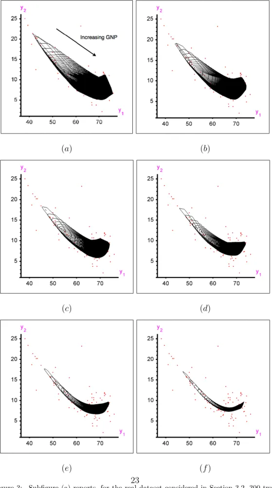
Figure 3(a) reports, in a single two-dimensional picture, the 300 cuts of the (τ = 0.10)-quantile regression contour that are associated withz0 = 100,

200, 300, . . . ,29900,and 30000. Figures 3(b)-(f) show the corresponding cuts computed from the quantile regions with orderτ = 0.15, 0.20, 0.25, 0.30, and 0.35, respectively. Clearly, these cuts provide interesting information about the trend (for high values of τ) and about the shape (for low values of τ).

4. Simulations

We now present some empirical results that quantify the speed (and show the possibilities) of our Matlabimplementation of the procedure described in this paper. We used an Apple computer with Intel Core Duo 1.83GHz, 512MB RAM, Win XPSP2 and Matlab 7.3.0.267. Of course, other hard-ware or initial settings (see the Appendix) may lead to different results.

4.1. Speed comparison

In the location case (p = 1), the quantile regions provided by our code coincide with the halfspace depth contours. As already mentioned, there is no exact implementable algorithm that could be used as a competitor to our code for m > 2. For the bivariate case (m = 2), however, we can compare our _Matlab code with that coauthored and kindly provided to us by Ivan Mizera that we chose for a benchmark.

In order to do so, we generated n i.i.d. bivariate observations (i) from the bivariate standard normal distibution N(0,1)2 _{(S = 1) and (ii) from the}

(a) (b)

(c) (d)

(e) (f)

Figure 3: Subfigure (a) reports, for the real dataset considered in Section 3.2, 300 two-dimensional cuts (each associated with one fixed value of GNP per capita) of the (four-dimensional) quantile regions of orderτ = 0.10. Subfigure (b)-(f) show the corresponding plots for τ = 0.15, 0.20, 0.25, 0.30, and 0.35, respectively; we refer to Section 3.2 for

centered bivariate uniform distribution over the unit square U([−0.5,0.5])2

(S = 2). For any combination ofτ ={0.010, 0.025, 0.050, 0.100, 0.200, 0.300, 0.400} and n ∈ {50,100,150,200,250,300,500,1000,2000,5000,10000,

20000}, we ran the computation ten times for each scenario S3. Average execution times in seconds are reported in Table 1 and show that the com-putation hardly takes more than 2 minutes even for n= 10000.

We should point out that the comparison with the benchmark should be interpreted with care as each program leads to different output. Our code produces halfspaces whose intersection equals the sample halfspace depth region. Therefore they can be used straightforwardly for identifying points inside, on, or outside the contours. On the other hand, the benchmark leads to the vertices of the halfspace depth region and identifies its inner points (we do not know the details). Both representations may be useful but a vertex-facet or vertex-facet-vertex enumeration method has to be used for converting one into the other. Besides, it should be kept in mind that our code provides enough material for computing two neighbouring contours at once (see the comments below the proofs of Theorem 4.2 in HPˇS10) while the benchmark does not.

3_{Actually, with the following changes to the default settings of our code:}

CTechST.InCheckI = 0, CTechST.ReportI = 0, CTechST.TestModeI = 0, and CTechST.OutSaveI = 0. This suppresses checking the input for correctness, detailed output on the screen, computing some auxiliary technical statistics and storing the output on the disk, all that to make our code faster and possible to use in an extensive simulation. Note that the output form= 2 andn≤10000 is usually small enough to be kept in the internal memory; so the last option does not affect the results too much here.

It should also be noted that our study does not compare the algorithms but only their implementations. The benchmark has originally been devel-oped only for auxiliary validation, with no speed optimization in mind. On the other hand, our search for the first optimal solution is not likely to be the fastest possible as well.

Despite the limitations of this comparison, the results seem to demon-strate high stability and superiority of our code because it was always ob-served faster than the benchmark, sometimes even more than 16 times. It excells especially when applied to medium-sized data sets and not too ex-treme values of τ.

The decrease of relative efficiency of our code for very small values of τ

or n can be explained by the fact that it is the slow finding of the initial solution that contributes the most to the overall execution time in these cases. Indeed, profiling of the code in Matlab shows that this contribution is usually higher than 30% even for n = 5000 if τ = 0.01 (and exceeds 75% for n = 50 and the same τ). On the other hand, if τ = 0.3, then this contribution is still often larger than 30% for n = 50 but usually drops below 5% for n = 5000. Different memory space requirements may also play some role, especially if n is set very high.

4.2. General regression case

Next we consider the general regression context represented by the simple model

Yp×1 =Bp×mXm×1+εp×1,

where X1 = 1, (X2, . . . , Xp)0 has i.i.d. marginals that are uniformly

from the p×m matrix of ones by replacing the elements in the first column with zeros. Average execution times4 in seconds, for a total of rreplications, are recorded for many combinations ofn,pand τ in Table 2 (for m= 2 with

r = 10), in Table 3 (for m = 3 with r = 5, and for m ∈ {4,5} with r = 3), and in Table 4 that focuses on outlier detection (for m = 3 with r = 3 and with very low values of τ).

These results can be used by the reader for estimating the time require-ments of his/her own computation with our code. It appears that the compu-tation can hardly take more than some 18 minutes on average in the case of two-dimensional responses (m = 2), n ≤ 10000 and p ≤ 12. Unfortunately (but not surprisingly), the time requirements and the size of output grow with increasing dimension of the response. If m = 3, then the computation appears advantageous for 500 observations at most, perhaps except for some very low τ’s and p’s. If m >3, then it is hard to evaluate the correctness of the results. But it appears that all the halfspaces can still be computed in a reasonable time for a few hundreds of observations and extreme τ’s even in four and five dimensions, which might be employed for outlier identification. Virtually the same regression quantile regions can also be obtained from a competing directional quantile concept introduced in Kong and Mizera (2008); see Theorem 4.3 in Paindaveine and ˇSiman (2010a). Therefore, it makes sense to use as a competitor here the Matlabimplementation for this competing concept proposed in Paindaveine and ˇSiman (2010b).

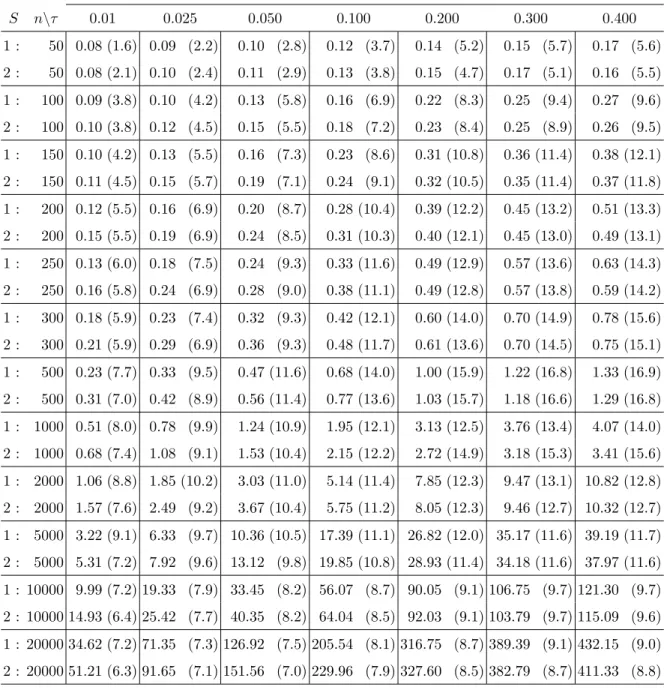
Absolute and relative execution times S n\τ 0.01 0.025 0.050 0.100 0.200 0.300 0.400 1 : 50 0.08 (1.6) 0.09 (2.2) 0.10 (2.8) 0.12 (3.7) 0.14 (5.2) 0.15 (5.7) 0.17 (5.6) 2 : 50 0.08 (2.1) 0.10 (2.4) 0.11 (2.9) 0.13 (3.8) 0.15 (4.7) 0.17 (5.1) 0.16 (5.5) 1 : 100 0.09 (3.8) 0.10 (4.2) 0.13 (5.8) 0.16 (6.9) 0.22 (8.3) 0.25 (9.4) 0.27 (9.6) 2 : 100 0.10 (3.8) 0.12 (4.5) 0.15 (5.5) 0.18 (7.2) 0.23 (8.4) 0.25 (8.9) 0.26 (9.5) 1 : 150 0.10 (4.2) 0.13 (5.5) 0.16 (7.3) 0.23 (8.6) 0.31 (10.8) 0.36 (11.4) 0.38 (12.1) 2 : 150 0.11 (4.5) 0.15 (5.7) 0.19 (7.1) 0.24 (9.1) 0.32 (10.5) 0.35 (11.4) 0.37 (11.8) 1 : 200 0.12 (5.5) 0.16 (6.9) 0.20 (8.7) 0.28 (10.4) 0.39 (12.2) 0.45 (13.2) 0.51 (13.3) 2 : 200 0.15 (5.5) 0.19 (6.9) 0.24 (8.5) 0.31 (10.3) 0.40 (12.1) 0.45 (13.0) 0.49 (13.1) 1 : 250 0.13 (6.0) 0.18 (7.5) 0.24 (9.3) 0.33 (11.6) 0.49 (12.9) 0.57 (13.6) 0.63 (14.3) 2 : 250 0.16 (5.8) 0.24 (6.9) 0.28 (9.0) 0.38 (11.1) 0.49 (12.8) 0.57 (13.8) 0.59 (14.2) 1 : 300 0.18 (5.9) 0.23 (7.4) 0.32 (9.3) 0.42 (12.1) 0.60 (14.0) 0.70 (14.9) 0.78 (15.6) 2 : 300 0.21 (5.9) 0.29 (6.9) 0.36 (9.3) 0.48 (11.7) 0.61 (13.6) 0.70 (14.5) 0.75 (15.1) 1 : 500 0.23 (7.7) 0.33 (9.5) 0.47 (11.6) 0.68 (14.0) 1.00 (15.9) 1.22 (16.8) 1.33 (16.9) 2 : 500 0.31 (7.0) 0.42 (8.9) 0.56 (11.4) 0.77 (13.6) 1.03 (15.7) 1.18 (16.6) 1.29 (16.8) 1 : 1000 0.51 (8.0) 0.78 (9.9) 1.24 (10.9) 1.95 (12.1) 3.13 (12.5) 3.76 (13.4) 4.07 (14.0) 2 : 1000 0.68 (7.4) 1.08 (9.1) 1.53 (10.4) 2.15 (12.2) 2.72 (14.9) 3.18 (15.3) 3.41 (15.6) 1 : 2000 1.06 (8.8) 1.85 (10.2) 3.03 (11.0) 5.14 (11.4) 7.85 (12.3) 9.47 (13.1) 10.82 (12.8) 2 : 2000 1.57 (7.6) 2.49 (9.2) 3.67 (10.4) 5.75 (11.2) 8.05 (12.3) 9.46 (12.7) 10.32 (12.7) 1 : 5000 3.22 (9.1) 6.33 (9.7) 10.36 (10.5) 17.39 (11.1) 26.82 (12.0) 35.17 (11.6) 39.19 (11.7) 2 : 5000 5.31 (7.2) 7.92 (9.6) 13.12 (9.8) 19.85 (10.8) 28.93 (11.4) 34.18 (11.6) 37.97 (11.6) 1 : 10000 9.99 (7.2) 19.33 (7.9) 33.45 (8.2) 56.07 (8.7) 90.05 (9.1) 106.75 (9.7) 121.30 (9.7) 2 : 10000 14.93 (6.4) 25.42 (7.7) 40.35 (8.2) 64.04 (8.5) 92.03 (9.1) 103.79 (9.7) 115.09 (9.6) 1 : 20000 34.62 (7.2) 71.35 (7.3) 126.92 (7.5) 205.54 (8.1) 316.75 (8.7) 389.39 (9.1) 432.15 (9.0) 2 : 20000 51.21 (6.3) 91.65 (7.1) 151.56 (7.0) 229.96 (7.9) 327.60 (8.5) 382.79 (8.7) 411.33 (8.8)

Table 1: (2D location settings: m = 2 and p= 1) Average execution time (in seconds) of our code is provided for given scenario S, number of observations n, and order τ in the bivariate location context. The numbers in parentheses indicate how many times it is faster than the benchmark.

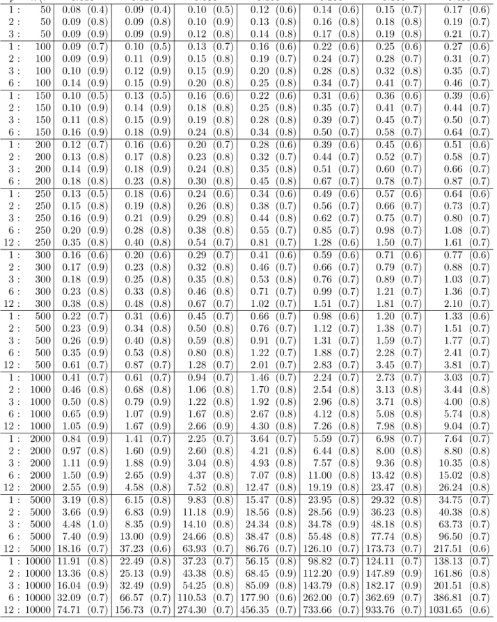
Absolute and relative execution times p n\τ 0.010 0.025 0.050 0.100 0.200 0.300 0.400 1 : 50 0.08 (0.4) 0.09 (0.4) 0.10 (0.5) 0.12 (0.6) 0.14 (0.6) 0.15 (0.7) 0.17 (0.6) 2 : 50 0.09 (0.8) 0.09 (0.8) 0.10 (0.9) 0.13 (0.8) 0.16 (0.8) 0.18 (0.8) 0.19 (0.7) 3 : 50 0.09 (0.9) 0.09 (0.9) 0.12 (0.8) 0.14 (0.8) 0.17 (0.8) 0.19 (0.8) 0.21 (0.7) 1 : 100 0.09 (0.7) 0.10 (0.5) 0.13 (0.7) 0.16 (0.6) 0.22 (0.6) 0.25 (0.6) 0.27 (0.6) 2 : 100 0.09 (0.9) 0.11 (0.9) 0.15 (0.8) 0.19 (0.7) 0.24 (0.7) 0.28 (0.7) 0.31 (0.7) 3 : 100 0.10 (0.9) 0.12 (0.9) 0.15 (0.9) 0.20 (0.8) 0.28 (0.8) 0.32 (0.8) 0.35 (0.7) 6 : 100 0.14 (0.9) 0.15 (0.9) 0.20 (0.8) 0.25 (0.8) 0.34 (0.7) 0.41 (0.7) 0.46 (0.7) 1 : 150 0.10 (0.5) 0.13 (0.5) 0.16 (0.6) 0.22 (0.6) 0.31 (0.6) 0.36 (0.6) 0.39 (0.6) 2 : 150 0.10 (0.9) 0.14 (0.9) 0.18 (0.8) 0.25 (0.8) 0.35 (0.7) 0.41 (0.7) 0.44 (0.7) 3 : 150 0.11 (0.8) 0.15 (0.9) 0.19 (0.8) 0.28 (0.8) 0.39 (0.7) 0.45 (0.7) 0.50 (0.7) 6 : 150 0.16 (0.9) 0.18 (0.9) 0.24 (0.8) 0.34 (0.8) 0.50 (0.7) 0.58 (0.7) 0.64 (0.7) 1 : 200 0.12 (0.7) 0.16 (0.6) 0.20 (0.7) 0.28 (0.6) 0.39 (0.6) 0.45 (0.6) 0.51 (0.6) 2 : 200 0.13 (0.8) 0.17 (0.8) 0.23 (0.8) 0.32 (0.7) 0.44 (0.7) 0.52 (0.7) 0.58 (0.7) 3 : 200 0.14 (0.9) 0.18 (0.9) 0.24 (0.8) 0.35 (0.8) 0.51 (0.7) 0.60 (0.7) 0.66 (0.7) 6 : 200 0.18 (0.8) 0.23 (0.8) 0.30 (0.8) 0.45 (0.8) 0.67 (0.7) 0.78 (0.7) 0.87 (0.7) 1 : 250 0.13 (0.5) 0.18 (0.6) 0.24 (0.6) 0.34 (0.6) 0.49 (0.6) 0.57 (0.6) 0.64 (0.6) 2 : 250 0.15 (0.8) 0.19 (0.8) 0.26 (0.8) 0.38 (0.7) 0.56 (0.7) 0.66 (0.7) 0.73 (0.7) 3 : 250 0.16 (0.9) 0.21 (0.9) 0.29 (0.8) 0.44 (0.8) 0.62 (0.7) 0.75 (0.7) 0.80 (0.7) 6 : 250 0.20 (0.9) 0.28 (0.8) 0.38 (0.8) 0.55 (0.7) 0.85 (0.7) 0.98 (0.7) 1.08 (0.7) 12 : 250 0.35 (0.8) 0.40 (0.8) 0.54 (0.7) 0.81 (0.7) 1.28 (0.6) 1.50 (0.7) 1.61 (0.7) 1 : 300 0.16 (0.6) 0.20 (0.6) 0.29 (0.7) 0.41 (0.6) 0.59 (0.6) 0.71 (0.6) 0.77 (0.6) 2 : 300 0.17 (0.9) 0.23 (0.8) 0.32 (0.8) 0.46 (0.7) 0.66 (0.7) 0.79 (0.7) 0.88 (0.7) 3 : 300 0.18 (0.9) 0.25 (0.8) 0.35 (0.8) 0.53 (0.8) 0.76 (0.7) 0.89 (0.7) 1.03 (0.7) 6 : 300 0.23 (0.8) 0.33 (0.8) 0.46 (0.8) 0.71 (0.7) 0.99 (0.7) 1.21 (0.7) 1.36 (0.7) 12 : 300 0.38 (0.8) 0.48 (0.8) 0.67 (0.7) 1.02 (0.7) 1.51 (0.7) 1.81 (0.7) 2.10 (0.7) 1 : 500 0.22 (0.7) 0.31 (0.6) 0.45 (0.7) 0.66 (0.7) 0.98 (0.6) 1.20 (0.7) 1.33 (0.6) 2 : 500 0.23 (0.9) 0.34 (0.8) 0.50 (0.8) 0.76 (0.7) 1.12 (0.7) 1.38 (0.7) 1.51 (0.7) 3 : 500 0.26 (0.9) 0.40 (0.8) 0.59 (0.8) 0.91 (0.7) 1.31 (0.7) 1.59 (0.7) 1.77 (0.7) 6 : 500 0.35 (0.9) 0.53 (0.8) 0.80 (0.8) 1.22 (0.7) 1.88 (0.7) 2.28 (0.7) 2.41 (0.7) 12 : 500 0.61 (0.7) 0.87 (0.7) 1.28 (0.7) 2.01 (0.7) 2.83 (0.7) 3.45 (0.7) 3.81 (0.7) 1 : 1000 0.41 (0.7) 0.61 (0.7) 0.94 (0.7) 1.46 (0.7) 2.24 (0.7) 2.73 (0.7) 3.03 (0.7) 2 : 1000 0.46 (0.8) 0.68 (0.8) 1.06 (0.8) 1.70 (0.8) 2.54 (0.8) 3.13 (0.8) 3.44 (0.8) 3 : 1000 0.50 (0.8) 0.79 (0.9) 1.22 (0.8) 1.92 (0.8) 2.96 (0.8) 3.71 (0.8) 4.00 (0.8) 6 : 1000 0.65 (0.9) 1.07 (0.9) 1.67 (0.8) 2.67 (0.8) 4.12 (0.8) 5.08 (0.8) 5.74 (0.8) 12 : 1000 1.05 (0.9) 1.67 (0.9) 2.66 (0.9) 4.30 (0.8) 7.26 (0.8) 7.98 (0.8) 9.04 (0.7) 1 : 2000 0.84 (0.9) 1.41 (0.7) 2.25 (0.7) 3.64 (0.7) 5.59 (0.7) 6.98 (0.7) 7.64 (0.7) 2 : 2000 0.97 (0.8) 1.60 (0.9) 2.60 (0.8) 4.21 (0.8) 6.44 (0.8) 8.00 (0.8) 8.80 (0.8) 3 : 2000 1.11 (0.9) 1.88 (0.9) 3.04 (0.8) 4.93 (0.8) 7.57 (0.8) 9.36 (0.8) 10.35 (0.8) 6 : 2000 1.50 (0.9) 2.65 (0.9) 4.37 (0.8) 7.07 (0.8) 11.00 (0.8) 13.42 (0.8) 15.02 (0.8) 12 : 2000 2.55 (0.9) 4.58 (0.8) 7.52 (0.8) 12.47 (0.8) 19.19 (0.8) 23.47 (0.8) 26.24 (0.8) 1 : 5000 3.19 (0.8) 6.15 (0.8) 9.83 (0.8) 15.47 (0.8) 23.95 (0.8) 29.32 (0.8) 34.75 (0.7) 2 : 5000 3.66 (0.9) 6.83 (0.9) 11.18 (0.9) 18.56 (0.8) 28.56 (0.9) 36.23 (0.8) 40.38 (0.8) 3 : 5000 4.48 (1.0) 8.35 (0.9) 14.10 (0.8) 24.34 (0.8) 34.78 (0.9) 48.18 (0.8) 63.73 (0.7) 6 : 5000 7.40 (0.9) 13.00 (0.9) 24.66 (0.8) 38.47 (0.8) 55.48 (0.8) 77.74 (0.8) 96.50 (0.7) 12 : 5000 18.16 (0.7) 37.23 (0.6) 63.93 (0.7) 86.76 (0.7) 126.10 (0.7) 173.73 (0.7) 217.51 (0.6) 1 : 10000 11.91 (0.8) 22.49 (0.8) 37.23 (0.7) 56.15 (0.8) 98.82 (0.7) 124.11 (0.7) 138.13 (0.7) 2 : 10000 13.36 (0.8) 25.13 (0.9) 43.38 (0.8) 68.45 (0.9) 112.20 (0.9) 147.89 (0.9) 161.86 (0.8) 3 : 10000 16.04 (0.9) 32.49 (0.9) 54.25 (0.8) 85.09 (0.8) 143.79 (0.8) 182.17 (0.9) 201.51 (0.8) 6 : 10000 32.09 (0.7) 66.57 (0.7) 110.53 (0.7) 177.90 (0.6) 262.00 (0.7) 362.69 (0.7) 386.81 (0.7) 12 : 10000 74.71 (0.7) 156.73 (0.7) 274.30 (0.7) 456.35 (0.7) 733.66 (0.7) 933.76 (0.7) 1031.65 (0.6)

Table 2: (2D regression settings: m= 2) Average execution time (in seconds) of our code, based onr= 10 replications, is provided for quantile orderτ,pregressors (including the intercept) and nobservations. The numbers in parentheses indicate how many times it is28

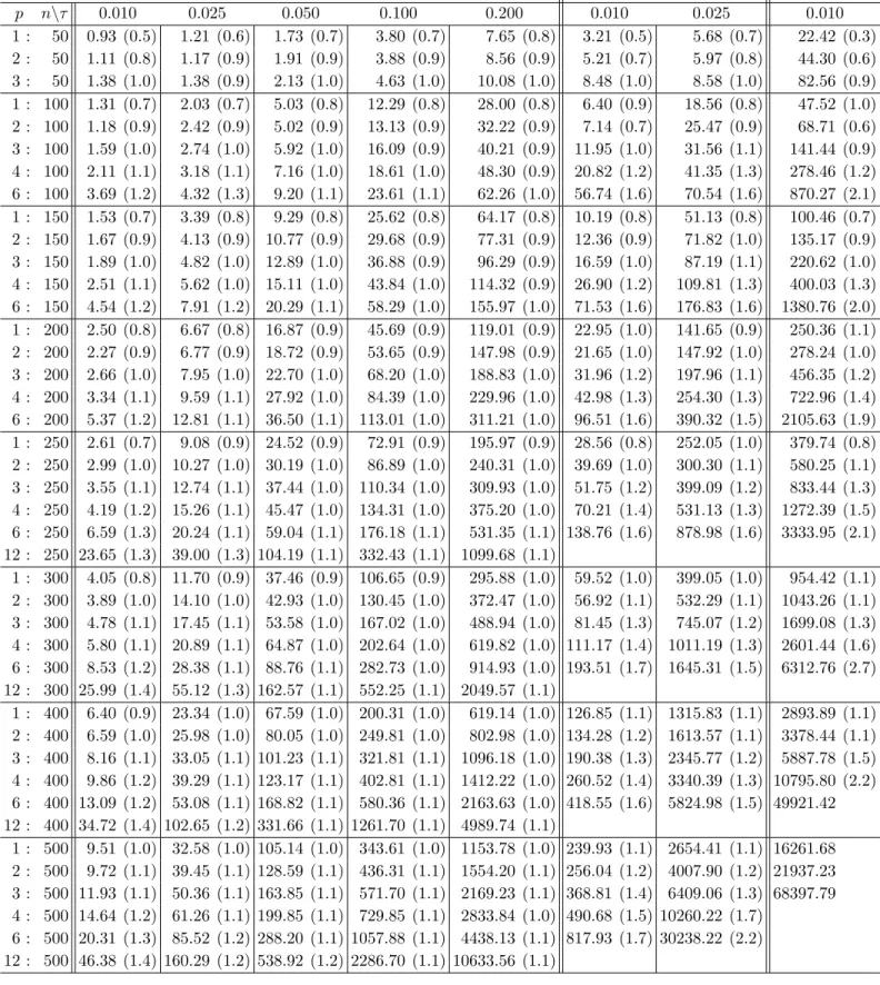
Absolute and relative execution times m= 3 m= 4 m= 5 p n\τ 0.010 0.025 0.050 0.100 0.200 0.010 0.025 0.010 1 : 50 0.93 (0.5) 1.21 (0.6) 1.73 (0.7) 3.80 (0.7) 7.65 (0.8) 3.21 (0.5) 5.68 (0.7) 22.42 (0.3) 2 : 50 1.11 (0.8) 1.17 (0.9) 1.91 (0.9) 3.88 (0.9) 8.56 (0.9) 5.21 (0.7) 5.97 (0.8) 44.30 (0.6) 3 : 50 1.38 (1.0) 1.38 (0.9) 2.13 (1.0) 4.63 (1.0) 10.08 (1.0) 8.48 (1.0) 8.58 (1.0) 82.56 (0.9) 1 : 100 1.31 (0.7) 2.03 (0.7) 5.03 (0.8) 12.29 (0.8) 28.00 (0.8) 6.40 (0.9) 18.56 (0.8) 47.52 (1.0) 2 : 100 1.18 (0.9) 2.42 (0.9) 5.02 (0.9) 13.13 (0.9) 32.22 (0.9) 7.14 (0.7) 25.47 (0.9) 68.71 (0.6) 3 : 100 1.59 (1.0) 2.74 (1.0) 5.92 (1.0) 16.09 (0.9) 40.21 (0.9) 11.95 (1.0) 31.56 (1.1) 141.44 (0.9) 4 : 100 2.11 (1.1) 3.18 (1.1) 7.16 (1.0) 18.61 (1.0) 48.30 (0.9) 20.82 (1.2) 41.35 (1.3) 278.46 (1.2) 6 : 100 3.69 (1.2) 4.32 (1.3) 9.20 (1.1) 23.61 (1.1) 62.26 (1.0) 56.74 (1.6) 70.54 (1.6) 870.27 (2.1) 1 : 150 1.53 (0.7) 3.39 (0.8) 9.29 (0.8) 25.62 (0.8) 64.17 (0.8) 10.19 (0.8) 51.13 (0.8) 100.46 (0.7) 2 : 150 1.67 (0.9) 4.13 (0.9) 10.77 (0.9) 29.68 (0.9) 77.31 (0.9) 12.36 (0.9) 71.82 (1.0) 135.17 (0.9) 3 : 150 1.89 (1.0) 4.82 (1.0) 12.89 (1.0) 36.88 (0.9) 96.29 (0.9) 16.59 (1.0) 87.19 (1.1) 220.62 (1.0) 4 : 150 2.51 (1.1) 5.62 (1.0) 15.11 (1.0) 43.84 (1.0) 114.32 (0.9) 26.90 (1.2) 109.81 (1.3) 400.03 (1.3) 6 : 150 4.54 (1.2) 7.91 (1.2) 20.29 (1.1) 58.29 (1.0) 155.97 (1.0) 71.53 (1.6) 176.83 (1.6) 1380.76 (2.0) 1 : 200 2.50 (0.8) 6.67 (0.8) 16.87 (0.9) 45.69 (0.9) 119.01 (0.9) 22.95 (1.0) 141.65 (0.9) 250.36 (1.1) 2 : 200 2.27 (0.9) 6.77 (0.9) 18.72 (0.9) 53.65 (0.9) 147.98 (0.9) 21.65 (1.0) 147.92 (1.0) 278.24 (1.0) 3 : 200 2.66 (1.0) 7.95 (1.0) 22.70 (1.0) 68.20 (1.0) 188.83 (1.0) 31.96 (1.2) 197.96 (1.1) 456.35 (1.2) 4 : 200 3.34 (1.1) 9.59 (1.1) 27.92 (1.0) 84.39 (1.0) 229.96 (1.0) 42.98 (1.3) 254.30 (1.3) 722.96 (1.4) 6 : 200 5.37 (1.2) 12.81 (1.1) 36.50 (1.1) 113.01 (1.0) 311.21 (1.0) 96.51 (1.6) 390.32 (1.5) 2105.63 (1.9) 1 : 250 2.61 (0.7) 9.08 (0.9) 24.52 (0.9) 72.91 (0.9) 195.97 (0.9) 28.56 (0.8) 252.05 (1.0) 379.74 (0.8) 2 : 250 2.99 (1.0) 10.27 (1.0) 30.19 (1.0) 86.89 (1.0) 240.31 (1.0) 39.69 (1.0) 300.30 (1.1) 580.25 (1.1) 3 : 250 3.55 (1.1) 12.74 (1.1) 37.44 (1.0) 110.34 (1.0) 309.93 (1.0) 51.75 (1.2) 399.09 (1.2) 833.44 (1.3) 4 : 250 4.19 (1.2) 15.26 (1.1) 45.47 (1.0) 134.31 (1.0) 375.20 (1.0) 70.21 (1.4) 531.13 (1.3) 1272.39 (1.5) 6 : 250 6.59 (1.3) 20.24 (1.1) 59.04 (1.1) 176.18 (1.1) 531.35 (1.1) 138.76 (1.6) 878.98 (1.6) 3333.95 (2.1) 12 : 250 23.65 (1.3) 39.00 (1.3) 104.19 (1.1) 332.43 (1.1) 1099.68 (1.1) 1 : 300 4.05 (0.8) 11.70 (0.9) 37.46 (0.9) 106.65 (0.9) 295.88 (1.0) 59.52 (1.0) 399.05 (1.0) 954.42 (1.1) 2 : 300 3.89 (1.0) 14.10 (1.0) 42.93 (1.0) 130.45 (1.0) 372.47 (1.0) 56.92 (1.1) 532.29 (1.1) 1043.26 (1.1) 3 : 300 4.78 (1.1) 17.45 (1.1) 53.58 (1.0) 167.02 (1.0) 488.94 (1.0) 81.45 (1.3) 745.07 (1.2) 1699.08 (1.3) 4 : 300 5.80 (1.1) 20.89 (1.1) 64.87 (1.0) 202.64 (1.0) 619.82 (1.0) 111.17 (1.4) 1011.19 (1.3) 2601.44 (1.6) 6 : 300 8.53 (1.2) 28.38 (1.1) 88.76 (1.1) 282.73 (1.0) 914.93 (1.0) 193.51 (1.7) 1645.31 (1.5) 6312.76 (2.7) 12 : 300 25.99 (1.4) 55.12 (1.3) 162.57 (1.1) 552.25 (1.1) 2049.57 (1.1) 1 : 400 6.40 (0.9) 23.34 (1.0) 67.59 (1.0) 200.31 (1.0) 619.14 (1.0) 126.85 (1.1) 1315.83 (1.1) 2893.89 (1.1) 2 : 400 6.59 (1.0) 25.98 (1.0) 80.05 (1.0) 249.81 (1.0) 802.98 (1.0) 134.28 (1.2) 1613.57 (1.1) 3378.44 (1.1) 3 : 400 8.16 (1.1) 33.05 (1.1) 101.23 (1.1) 321.81 (1.1) 1096.18 (1.0) 190.38 (1.3) 2345.77 (1.2) 5887.78 (1.5) 4 : 400 9.86 (1.2) 39.29 (1.1) 123.17 (1.1) 402.81 (1.1) 1412.22 (1.0) 260.52 (1.4) 3340.39 (1.3) 10795.80 (2.2) 6 : 400 13.09 (1.2) 53.08 (1.1) 168.82 (1.1) 580.36 (1.1) 2163.63 (1.0) 418.55 (1.6) 5824.98 (1.5) 49921.42 12 : 400 34.72 (1.4) 102.65 (1.2) 331.66 (1.1) 1261.70 (1.1) 4989.74 (1.1) 1 : 500 9.51 (1.0) 32.58 (1.0) 105.14 (1.0) 343.61 (1.0) 1153.78 (1.0) 239.93 (1.1) 2654.41 (1.1) 16261.68 2 : 500 9.72 (1.1) 39.45 (1.1) 128.59 (1.1) 436.31 (1.1) 1554.20 (1.1) 256.04 (1.2) 4007.90 (1.2) 21937.23 3 : 500 11.93 (1.1) 50.36 (1.1) 163.85 (1.1) 571.70 (1.1) 2169.23 (1.1) 368.81 (1.4) 6409.06 (1.3) 68397.79 4 : 500 14.64 (1.2) 61.26 (1.1) 199.85 (1.1) 729.85 (1.1) 2833.84 (1.0) 490.68 (1.5) 10260.22 (1.7) 6 : 500 20.31 (1.3) 85.52 (1.2) 288.20 (1.1) 1057.88 (1.1) 4438.13 (1.1) 817.93 (1.7) 30238.22 (2.2) 12 : 500 46.38 (1.4) 160.29 (1.2) 538.92 (1.2) 2286.70 (1.1) 10633.56 (1.1)

Table 3: (Multidimensional regression settings) Average execution time (in seconds) of our code, based on r = 5 replications if m = 3 and on r = 3 replications otherwise, is provided for quantile orderτ, pregressors (including the intercept) andn m-dimensional responses. The numbers in parentheses indicate how many times it is faster than the code

Absolute and relative execution times τ p\n 750 1000 1200 1500 2000 1 : 18.14 (1.1) 35.55 (1.2) 56.09 (1.3) 94.28 (1.4) 195.29 (1.5) 2 : 23.48 (1.2) 41.68 (1.3) 68.35 (1.3) 117.58 (1.4) 246.84 (1.5) 0.010 3 : 29.19 (1.2) 54.74 (1.3) 88.14 (1.3) 152.60 (1.4) 326.46 (1.5) 4 : 35.66 (1.2) 67.12 (1.3) 108.72 (1.3) 190.93 (1.4) 418.35 (1.4) 6 : 48.88 (1.3) 97.84 (1.3) 155.05 (1.2) 290.53 (1.3) 637.53 (1.4) 1 : 86.18 (1.1) 171.83 (1.2) 262.79 (1.3) 474.01 (1.4) 1058.50 (1.4) 2 : 109.89 (1.2) 210.19 (1.3) 328.72 (1.3) 623.02 (1.4) 1410.02 (1.4) 0.025 3 : 142.86 (1.2) 279.95 (1.2) 439.60 (1.3) 837.58 (1.3) 1913.23 (1.4) 4 : 174.72 (1.2) 344.79 (1.2) 561.45 (1.2) 1063.29 (1.3) 2519.76 (1.3) 6 : 249.20 (1.2) 512.89 (1.2) 836.57 (1.2) 1649.89 (1.2) 3914.40 (1.2) 1 : 294.01 (1.1) 593.70 (1.2) 1006.57 (1.2) 1968.37 (1.3) 4719.26 (1.3) 2 : 376.06 (1.2) 760.21 (1.2) 1328.50 (1.2) 2620.97 (1.3) 6531.65 (1.3) 0.050 3 : 496.03 (1.1) 1042.85 (1.2) 1834.28 (1.2) 3616.83 (1.3) 9239.28 (1.2) 4 : 619.62 (1.1) 1328.00 (1.2) 2400.54 (1.2) 4805.97 (1.2) 12477.26 (1.2) 6 : 924.38 (1.1) 2039.12 (1.1) 3700.73 (1.1) 7747.52 (1.2) 20362.39 (1.2) Table 4: (3D outlier detection: m= 3) Average execution time (in seconds) of our code, based on r= 3 replications, is provided for quantile order τ, pregressors (including the intercept) and n three-dimensional responses. The numbers in parentheses indicate how many times it is faster than the code from Paindaveine and ˇSiman (2010b).

Appendix A. Technical Details

In this section, we discuss some technical matters related to the algorithm described in this paper.

Choice ofτ. Ifnτ is an integer, then the linear programming problem (P) has infinitely many solutions for each u. If this complication occurs, we solve it by a small perturbation of τ, which can hardly make any important difference in most applications. Besides, there is only a finite number of different quantile regions anyway, so that such small perturbations ofτ could always be done without loss of generality when the goal is only to compute the quantile regions.

Input data. The code assumes m ∈ {2,3, . . . ,8} and n ≤ 100000 and its output should be quite reliable for m ∈ {2,3}, p ≤ 10 and n ≤ 10000 (if m = 2) or 500 (ifm = 3) at least. Now, the program was heavily tested only on data from our simulation study, with all coordinates less than 5 or so. This is why we strongly suggest to standardize the input observations in some way to a similar range whenever possible, which should enhance numerical stability of the algorithm. Besides, most real data are discrete because they are measured or recorded only with limited precision. This makes some bad data configurations more likely than almost impossible. Therefore we also recommend to perturb the input data points by some random noise of a reasonably small magnitude to prevent their discreteness from causing any trouble.

When a few identical observations occur, we may either aggregate the same rows of_AP into a single one or introduce (positive) weights intocP and

proceed analogously (the formulae would have to be changed a little but the crucial simplification of (DF) would persist). We prefer the first approach that is faster, easier to implement and still leads to the right quantile coeffi-cients. Since the algorithm does not rely on any special form ofxc₁, the code can also handle such aggregated or weighted rows (corresponding to weighted residuals). Therefore the program can be used even for bootstrap and sub-sampling methods quite easily. We might also refer to Hlubinka, Kot´ık and Venc´alek (2010) for another interesting attempt to combine weights with halfspace depth ideas.

Computing the first directional quantile. We decided to solve the prob-lem (P) with the aid of the freeMatlabtoolboxSeDuMi1.1 (see P´olik 2005 and Sturm 1999) that exploits sparsity and is very fast, flexible, and easy-to-use. Of course, any fast and reliable solver designed for univariate quantile regression might be substituted here.

As mentioned above, we can relax the assumptionu ∈ Sm−1 _{without any}

loss of generality because all non-zero vectorsu in the same direction lead to the same upper halfspace Hτ(nu)+. In general, we choose u0 as a normalized

corner of the hypercube [−1,1]m_{. Large or high-dimensional problems can}

be solved more effectively by segmenting the whole space to U0 regions of the

form

U0 ={u∈Rm : sign(u) = sign(u0)}

and considering each of these 2m _{different cube-like areas separately.}

If the starting direction leads to troubles, then other choices are tried until the optimal solution with the required number of non-zero coordinates is found.

Finding non-redundant constraints, facets and interior points. Ifm = 2, then the problem of finding non-redundant constraints and facets can be solved by assigning angles (say θ’s) to all the constraints in a clever way. The interior point can then be found simply by means of the facet normal vector.

For m > 2, the problem is far more complicated. First, we make the problem bounded by restricting to vectors u in [−1,1]m_{, which turns the}

cones from (5) into polytopes. Then we find all vertices and facets of such a polytope by means of the dual relationship between vertex and facet enu-meration (see Bremner, Fukuda, and Marzetta (1998)) and program qhull

(see Barber, Dobkin, and Huhdanpaa (1996)) for the latter one, fortunately accessible in Matlab (In fact, we only modify the function con2vert.m by Michael Kleder from Matlab Central File Exchange). This enumeration procedure requires an interior point of the resulting polytope to start. We search for it from the scaled centre of the known (parent) facet and in the direction of its normal vector.

In principle,uf might be found even without the artificial bounding with

subsequent vertex enumeration and the zero vertex problem might be ad-dressed as well; see Chv´atal (1983). However, we decided to tailor our code for qhull, which is an already developed and mature tool for solving similar problems that is quite stable, fast and familiar with rounding errors.

Realization of the breadth-first search algorithm. When this algorithm is employed, then some identifiers (scaled facet centres or facet normal vectors) of all (or lastly) used facets are stored in sorted archive(s) and a new facet is used for building the adjacent cone only if its identifier differs from all those

archived, which is checked by the binary search algorithm.

Plotting the contours. The program output describes the upper halfspaces whose intersection equals the quantile region of interest (if all of them are uniquely defined). Vertices of these regions could be obtained by the vertex enumeration mentioned above. The quantile contour with known vertices can be plotted easily by using _Matlab functionsconvhull orconvhulln. This is actually the procedure we used to generate all figures of the present paper.

Computing many (or all) contours at once. The first (initial) solutions could be found faster for all relevant τ’s at once than for each τ separately, by linear programming parametric inτ. In the purely location case, it would be advantageous to compute the contours from the highest τ < 0.5 to the lowest and to reduce the data set in each step (with adjustingτ accordingly), since inner points are redundant for computing outer contours. If we were interested even in the individual quantile hyperplanes and their coefficients in the general regression case, we could still replace all the surely interior observations with a single aggregated pseudo-observation keeping the new resulting subgradient conditions the same as before (as Roger Koenker kindly suggested to us). These proposals are not implemented in our code as it is designed to compute a single contour only.

Acknowledgement

The research work of Davy Paindaveine was supported by a Mandat d’Impulsion Scientifique of the Fonds National de la Recherche Scientifique, Communaut´e fran¸caise de Belgique. That of Miroslav ˇSiman was partly

sup-ported by achercheur postdoctoral temporaire contract of the Fonds National de la Recherche Scientifique, Communaut´e fran¸caise de Belgique, and partly by Project 1M06047 of the Ministry of Education, Youth and Sports of the Czech Republic. The authors would like to thank Roger Koenker and Ivan Mizera for inspiring discussions and advices. They also express their grati-tude to Ivan Mizera for kindly providing theMatlab code for computation of bivariate halfspace depth contours he coauthored with David Eppstein.

[1] Barber, C.B., Dobkin, D.P., and Huhdanpaa, H. (1996). The quickhull algorithm for convex hulls.ACM Transactions on Mathematical Software

22, 469–483.

[2] Bremner, D., Fukuda, K., and Marzetta, A. (1998). Primal-dual meth-ods for vertex and facet enumeration. Discrete and Computational Ge-ometry 20, 333-357.

[3] Chakraborty, B. (2003). On multivariate quantile regression. Journal of Statistical Planning and Inference 110 109–132.

[4] Chaudhuri, P. (1996). On a geometric notion of quantiles for multivariate data. Journal of the American Statistical Association 91 862–872.

[5] Chv´atal, V. (1983). Linear programming. W.H. Freeman & co, New York.

[6] Hallin, M., Paindaveine, D., and ˇSiman, M. (2010). Multivariate quan-tiles and multiple-output regression quanquan-tiles: From L1 optimization to

[7] Hlubinka, D., Kot´ık, L., and Venc´alek, O. (2010). Weighted halfspace depth. Kybernetika, to appear.

[8] Koenker, R. (2005). Quantile Regression. Cambridge University Press, New York, 1st edition.

[9] Koenker, R. (2007). Quantile regression in R: A vignette. Freely down-loadable from CRAN: http://cran.r-project.org.

[10] Koenker, R., and Bassett, G. J. (1978). Regression quantiles. Econo-metrica 46 33–50.

[11] Kon-Popovska, M. (2003). On some aspects of the matrix data pertur-bation in linear program. Yugoslav Journal of Operations Research 13, 153–164.

[12] Koltchinskii, V. (1997). M-estimation, convexity and quantiles. Ann. Statist. 25 435–477.

[13] Kong, L. and Mizera, I. (2008). Quantile tomography: using quantiles with multivariate data. Submitted. http://arxiv.org/abs/0805.0056.

[14] Lukas, M.A. and Shi, M. (2006). Sensitivity analysis of constrained linear

L1 regression: perturbations to constraints, addition and deletion of

observations. Computational Statistics & Data Analysis 51, 1213–1231

[15] Narula, S.C. and Wellington, J.F. (2002). Sensitivity analysis for predic-tor variables in the MSAE regression. Computational Statistics & Data Analysis 40, 355–373.

[16] Paindaveine, D. and ˇSiman, M. (2010a). On directional multiple-output quantile regression. Submitted.

[17] Paindaveine, D. and ˇSiman, M. (2010b). Computing all directional re-gression quantiles II. Manuscript in preparation.

[18] P´olik, I. (2005). Addendum to the SeDuMi user guide: Version 1.1.

[19] Rakovi´c, S.V., Grieder, P., and Jones, C. (2004). Computation of Voronoi diagrams and Delaunay triangulation via parametric linear pro-gramming. ETH Technical Report AUT04-03.

[20] Rouncefield, Mary (1995). The Statistics of Poverty and Inequality.

Journal of Statistics Education 3.

[21] Rousseeuw, P. J. and Ruts, I. (1999). The depth function of a population distribution. Metrika, 49, 213-244.

[22] Shi, M. and Lukas, M.A. (2005). Sensitivity analysis of constrained lin-ear L1 regression: perturbations to response and predictor variables. Computational Statistics & Data Analysis 48, 779–802.

[23] Sturm, J.F. (1999). Using SeDuMi 1.02, a_Matlabtoolbox for optimiza-tion over symmetric cones. Optimization Methods and Software 11-12, 625–653.

[24] Tukey, J. W. (1975). Mathematics and the picturing of data. In Proceed-ings of the international congress of mathematicians (Vancouver, B. C., 1974), Vol. 2, Quebec: Canad. Math. Congress 523–531.

[25] Wei, Y. (2008). An approach to multivariate covariate-dependent quan-tile contours with application to bivariate conditional growth charts. J. Amer. Statist. Assoc., 103, 397-409.