NBER WORKING PAPER SERIES
OPTIMAL SIMPLE AND IMPLEMENTABLE MONETARY AND FISCAL RULES: EXPANDED VERSION
Stephanie Schmitt-Grohé Martín Uribe Working Paper 12402
http://www.nber.org/papers/w12402
NATIONAL BUREAU OF ECONOMIC RESEARCH 1050 Massachusetts Avenue
Cambridge, MA 02138 July 2006
This paper is a substantially revised and expanded version of “Optimal Simple and Implementable Monetary and Fiscal Rules,” NBER working paper 10253, January 2004. A novel aspect of this revision is that it computes the Ramsey-optimal policy and uses it as the point of comparison for policy evaluation. We thank for comments an anonymous referee, Tommaso Monacelli, Robert Kollmann, Lars Svensson, and seminar participants at University Bocconi, the Bank of Italy, the CEPR-INSEAD Workshop on Monetary Policy Effectiveness, and Banco de la República (Bogotá, Colombia). The views expressed herein are those of the author(s) and do not necessarily reflect the views of the National Bureau of Economic Research.
©2006 by Stephanie Schmitt-Grohé and Martín Uribe. All rights reserved. Short sections of text, not to exceed two paragraphs, may be quoted without explicit permission provided that full credit, including © notice, is given to the source.
Optimal Simple and Implementable Monetary and Fiscal Rules: Expanded Version Stephanie Schmitt-Grohé and Martín Uribe
NBER Working Paper No. 12402 July 2006
JEL No. E52, E61, E63
ABSTRACT
This paper computes welfare-maximizing monetary and fiscal policy rules in a real business cycle model augmented with sticky prices, a demand for money, taxation, and stochastic government consumption. We consider simple feedback rules whereby the nominal interest rate is set as a function of output and inflation, and taxes are set as a function of total government liabilities. We implement a second-order accurate solution to the model. Our main findings are: First, the size of the inflation coefficient in the interest-rate rule plays a minor role for welfare. It matters only insofar as it affects the determinacy of equilibrium. Second, optimal monetary policy features a muted response to output. More importantly, interest rate rules that feature a positive response to output can lead to significant welfare losses. Third, the welfare gains from interest-rate smoothing are negligible. Fourth, optimal fiscal policy is passive. Finally, the optimal monetary and fiscal rule combination attains virtually the same level of welfare as the Ramsey optimal policy.
Stephanie Schmitt-Grohé Department of Economics Duke University P.O. Box 90097 Durham, NC 27708 and NBER [email protected] Martín Uribe Department of Economics Duke University Durham, NC 27708-0097 [email protected]
1
Introduction
Recently, there has been an outburst of papers studying optimal monetary policy in economies with nominal rigidities.1 Most of these studies are conducted in the context of highly stylized theoretical and policy environments. For instance, in much of this body of work it is assumed that the government has access to a subsidy to factor inputs, financed with lump-sum taxes, aimed at dismantling the inefficiency introduced by imperfect competition in product and factor markets. This assumption is clearly empirically unrealistic. But more importantly it undermines a potentially significant role for monetary policy, namely, stabilization of costly aggregate fluctuations around a distorted steady-state equilibrium.
A second notable simplification is the absence of capital accumulation. All the way from the work of Keynes (1936) and Hicks (1939) to that of Kydland and Prescott (1982) macroeconomic theories have emphasized investment dynamics as an important channel for the transmission of aggregate disturbances. It is therefore natural to expect that investment spending should play a role in shaping optimal monetary policy. Indeed it has been shown, that for a given monetary regime the determinacy properties of a standard Neo-Keynesian model can change dramatically when the assumption of capital accumulation is added to the model (Dupor, 2001; Carlstrom and Fuerst, 2005).
A third important dimension along which the existing studies abstract from reality is the assumed fiscal regime. It is standard practice in this literature to completely ignore fiscal policy. Implicitly, these models assume that the fiscal budget is balanced at all times by means of lump-sum taxation. In other words, fiscal policy is always assumed to be non-distorting and passive in the sense of Leeper (1991). However, empirical studies, such as Favero and Monacelli (2003), show that characterizing postwar U.S. fiscal policy as passive at all times is at odds with the facts. In addition, it is well known theoretically that, given monetary policy, the determinacy properties of the rational expectations equilibrium crucially depend on the nature of fiscal policy (e.g., Leeper, 1991). It follows that the design of optimal monetary policy should depend upon the underlying fiscal regime in a nontrivial fashion.
Fourth, model-based analyses of optimal monetary policy is typically restricted to economies in which long-run inflation is nil or there is some form of wide-spread indexation. As a re-sult, in the standard environments studied in the literature nominal rigidities have no real consequences for economic activity and thus welfare in the long-run. It follows that the assumptions of zero long-run inflation or indexation should not be expected to be inconse-1See Rotemberg and Woodford (1997, 1999), Clarida, Gal´ı, and Gertler (1999), Gal´ı and Monacelli (2005),
quential for the form that optimal monetary policy takes. Because from an empirical point of view, neither of these two assumptions is particularly compelling for economies like the United States, it is of interest to investigate the characteristics of optimal policy in their absence.
Last but not least, more often than not studies of optimal policy in models with nominal rigidities are conducted in cashless environments.2 This assumption introduces an inflation-stabilization bias into optimal monetary policy. For the presence of a demand for money creates a motive to stabilize the nominal interest rate rather than inflation.
Taken together the simplifying assumptions discussed above imply that business cycles are centered around an efficient non-distorted equilibrium. The main reason why these rather unrealistic features have been so widely adopted is not that they are the most empirically obvious ones to make nor that researchers believe that they are inconsequential for the nature of optimal monetary policy. Rather, the motivation is purely technical. Namely, the stylized models considered in the literature make it possible for a first-order approximation to the equilibrium conditions to be sufficient to accurately approximate welfare up to second order. Any plausible departure from the set of simplifying assumptions mentioned above, with the exception of the assumption of no investment dynamics, would require approximating the equilibrium conditions to second order.
Recent advances in computational economics have delivered algorithms that make it fea-sible and simple to compute higher-order approximations to the equilibrium conditions of a general class of large stochastic dynamic general equilibrium models.3 In this paper, we employ these new tools to analyze a model that relaxes all of the questionable assumptions mentioned above. The central focus of this paper is to investigate whether the policy conclu-sions arrived at by the existing literature regarding the optimal conduct of monetary policy are robust with respect to more realistic specifications of the economic environment. That is, we study optimal policy in a world where there are no subsidies to undo the distortions cre-ated by imperfect competition, where there is capital accumulation, where the government may follow active fiscal policy and may not have access to lump-sum taxation, where nom-inal rigidities induce inefficiencies even in the long run, and where there is a nonnegligible demand for money.
Specifically, this paper characterizes monetary and fiscal policy rules that are optimal within a family of implementable, simple rules in a calibrated model of the business cycle. In the model economy, business cycles are driven by stochastic variations in the level of total factor productivity and government consumption. The implementability condition requires
2Exceptions are Khan, King, and Wolman (2003) and Schmitt-Groh´e and Uribe (2004b). 3See, for instance, Schmitt-Groh´e and Uribe (2004a) and Sims (2000).
policies to deliver uniqueness of the rational expectations equilibrium. Simplicity requires restricting attention to rules whereby policy variables are set as a function of a small number of easily observable macroeconomic indicators. Specifically, we study interest-rate feedback rules that respond to measures of inflation, output and lagged values of the nominal interest rate. We analyze fiscal policy rules whereby the tax revenue is set as an increasing function of the level of public liabilities. The optimal simple and implementable rule is the simple and implementable rule that maximizes welfare of the individual agent. As a point of comparison for policy evaluation, we compute the real allocation associated with the Ramsey optimal policy.
Our findings suggest that the precise degree to which the central bank responds to in-flation in setting the nominal interest rate (i.e., the size of the inin-flation coefficient in the interest-rate rule) plays a minor role for welfare provided that the monetary/fiscal regime renders the equilibrium unique. For instance, in all of the many environments we consider, deviating from the optimal policy rule by setting the inflation coefficient anywhere above unity yields virtually the same level of welfare as the optimal rule. Thus, the fact that optimal policy features an active monetary stance serves mainly the purpose of ensuring the uniqueness of the rational expectations equilibrium. Second, optimal monetary policy features a muted response to output. More importantly, not responding to output is critical from a welfare point of view. In effect, our results show that interest rate rules that feature a positive response of the nominal interest rate to output can lead to significant welfare losses. Third, the welfare gains from interest-rate smoothing are negligible. Fourth, the optimal fiscal policy is passive. Finally, the optimal simple and implementable policy rule attains virtually the same level of welfare as the Ramsey optimal policy.
Kollmann (2003) also considers welfare maximizing fiscal and monetary rules in a sticky price model with capital accumulation. He also finds that optimal monetary policy features a strong anti-inflationary stance. However, the focus of his paper differs from ours in a number of dimensions. First, Kollmann does not consider the size of the welfare losses that are associated with non-optimal rules, which is at center stage in our work. Second, in his paper the interest rate feedback rule is not allowed to depend on a measure of aggregate activity and as a consequence the paper does not identify the importance of not responding to output. Third, Kollmann limits attention to a cashless economy with zero long run inflation. Finally, in Kollmann’s paper policy evaluation do not take the Ramsey optimal policy as the point of comparison.
The remainder of the paper is organized in six sections. Section 2 presents the model. Section 3 presents the calibration of the model and discusses computational issues. Section 4 computes optimal policy in a cashless economy. Section 5 analyzes optimal policy in a
monetary economy. Section 6 introduces fiscal instruments as part of the optimal policy design problem. Section 7 concludes.
2
The Model
The starting point for our investigation into the welfare consequences of alternative policy rules is an economic environment featuring a blend of neoclassical and neo-Keynesian ele-ments. Specifically, the skeleton of the economy is a standard real-business-cycle model with capital accumulation and endogenous labor supply driven by technology and government spending shocks. Five sources of inefficiency separate our model from the standard RBC framework: (a) nominal rigidities in the form of sluggish price adjustment. (b) A demand for money by firms motivated by a working-capital constraint on labor costs. (c) A demand for money by household originated in a cash-in-advance constraint. (d) monopolistic compe-tition in product markets. And (e) time-varying distortionary taxation. These five elements of the model provide a rationale for the conduct of monetary and fiscal stabilization policy.
2.1
Households
The economy is populated by a continuum of identical households. Each household has preferences defined over consumption, ct, and labor effort, ht. Preferences are described by
the utility function
E0
∞
X
t=0
βtU(ct, ht), (1)
where Et denotes the mathematical expectations operator conditional on information
avail-able at time t, β ∈ (0,1) represents a subjective discount factor, and U is a period utility index assumed to be strictly increasing in its first argument, strictly decreasing in its second argument, and strictly concave. The consumption good is assumed to be a composite good produced with a continuum of differentiated goods,cit,i∈[0,1], via the aggregator function
ct = Z 1 0 cit1−1/ηdi 1/(1−1/η) , (2)
where the parameter η > 1 denotes the intratemporal elasticity of substitution across dif-ferent varieties of consumption goods. For any given level of consumption of the composite good, purchases of each variety i in period t must solve the dual problem of minimizing total expenditure, R01Pitcitdi, subject to the aggregation constraint (2), where Pit denotes
the nominal price of a good of variety i at time t. The optimal level of cit is then given by cit= Pit Pt −η ct, (3)
where Pt is a nominal price index given by
Pt ≡ Z 1 0 Pit1−ηdi 1 1−η . (4)
This price index has the property that the minimum cost of a bundle of intermediate goods yielding ct units of the composite good is given byPtct.
Households are assumed to have access to a complete set of nominal contingent claims. Expenditures on consumption are subject to a cash-in-advance constraint of the form
mht ≥νhct, (5)
wheremh
t denotes real money holdings by the household in periodtandν
h ≥0 is a parameter.
The household’s period-by-period budget constraint is given by
Etdt,t+1 xt+1 Pt +mht +ct+it+τtL= xt Pt +Pt−1 Pt mht−1+ (1−τ D t )[wtht+utkt] +δq˜tτtDkt+ ˜φt, (6)
where dt,s is a stochastic discount factor, defined so that Etdt,sxs is the nominal value in
period t of a random nominal payment xs in periods ≥t. The variable kt denotes capital,
it denotes gross investment, ˜φt denotes profits received from the ownership of firms net of
income taxes,τtD denotes the income tax rate, and τ L
t denotes lump-sum taxes. The variable
˜
qt denotes the market price of one unit of installed capital. The term δτtDq˜tkt represents a
depreciation allowance for tax purposes. The capital stock is assumed to depreciate at the constant rate δ, and changes in the capital stock are assumed to be subject to a convex adjustment cost. The evolution of capital is given by
kt+1 = (1−δ)kt+itΨ it it−1 . (7)
The function Ψ is assumed to satisfy Ψ(1) = 1, Ψ0(1) = 0, and Ψ00(1)<0. These assumptions ensure no adjustment costs in the vicinity of the deterministic steady state. The investment good is assumed to be a composite good made with the aggregator function (2). Thus, the demand for each intermediate good i ∈ [0,1] for investment purposes, denoted iit, is
given by iit = (Pit/Pt)
−η
that prevents them from engaging in Ponzi schemes. The household’s problem consists in maximizing the utility function (1) subject to (5), (6), (7), and the no-Ponzi-game borrowing limit referred to above. Letting ζtλtβt, λtβt, and qtλtβt denote, respectively, the Lagrange
multipliers associated with (5), (6), and (7), the first-order conditions associated with the household’s problem are
Uc(ct, ht) =λt(1 +νhζt), (8) λtdt,t+1 =βλt+1 Pt Pt+1 −Uh(ct, ht) = wt(1−τtD)λt, (9) λt(1−ζt) =βEt λt+1 Pt Pt+1 (10) λt =λtqt Ψ it it−1 + it it−1 Ψ0 it it−1 −βEt ( λt+1qt+1 it+1 it 2 Ψ0 it+1 it ) (11) λtqt =βEtλt+1 (1−τtD+1)ut+1 +qt+1(1−δ) +δq˜t+1τtD+1 (12) ζt(mht −ν h ct) = 0 ζt ≥0
It is apparent from these first-order conditions that the income tax distorts both the leisure-labor choice and the decision to accumulate capital over time. At the same time, the oppor-tunity cost of holding money, 1/(1−ζt), which, as will become clear below equals the gross
nominal interest rate, distorts both the labor/leisure choice and the intertemporal allocation of consumption.
2.2
The Government
The consolidated government prints money, Mt, issues one-period nominally risk-free bonds,
Bt, collects taxes in the amount ofPtτt, and faces an exogenous expenditure stream,gt. Its
period-by-period budget constraint is given by
Mt+Bt =Rt−1Bt−1 +Mt−1+Ptgt−Ptτt.
Here Rt denotes the gross one-period, risk-free, nominal interest rate in period t. By a
no-arbitrage condition, Rt must equal the inverse of the period-t price of a portfolio that
pays one dollar in every state of period t + 1. That is, Rt = 1/Etdt,t+1. Combining this expression with the optimality conditions associated with the household’s problem yields
the usual Euler equation
λt =βRtEt
λt+1 πt+1
, (13)
where πt ≡ Pt/Pt−1 denotes the gross consumer price inflation. The variable gt denotes
per capita government spending on a composite good produced via the aggregator (2). We assume, maybe unrealistically, that the government minimizes the cost of producing gt.
Thus, we have that the public demand for each type i of intermediate goods,git, is given by
git = (Pit/Pt)
−η
gt.Let`t−1 ≡(Mt−1+Rt−1Bt−1)/Pt−1denote total real government liabilities outstanding at the end of period t−1 in units of period t−1 goods. Also, letmt ≡Mt/Pt
denote real money balances in circulation. Then the government budget constraint can be written as
`t =
Rt
πt
`t−1+Rt(gt−τt)−mt(Rt−1). (14)
We wish to consider various alternative fiscal policy specifications that involve possibly both lump sum and distortionary income taxation. Total tax revenues, τt, consist of revenue
from lump-sum taxation, τL
t , and revenue from income taxation, τ D
t yt, where yt denotes
aggregate demand.4 That is,
τt =τtL+τ D
t yt. (15)
The fiscal regime is defined by the following rule:
τt−τ∗ =γ1(`t−1 −`∗), (16)
whereγ1is a parameter, andτ∗ and`∗denote the deterministic Ramsey steady-state values of τt and`t, respectively. According to this rule, the fiscal authority sets tax revenues in period
t, τt, as a linear function of the real value of total government liabilities, `t−1. Combining
this fiscal rule with the government sequential budget constraint (14) yields
`t =
Rt
πt
(1−πtγ1)`t−1+Rt(γ1`∗ −τ∗) +Rtgt−mt(Rt−1).
When γ1 lies in the interval (0,2/π∗), we say, following the terminology of Leeper (1991), that fiscal policy is passive. Intuitively, in this case, in a stationary equilibrium near the deterministic steady state, deviations of real government liabilities from their nonstochastic steady-state level grow at a rate less than the real interest rate. As a result, the present 4In the economy with distortionary taxes only, we implicitly assume that profits are taxed in such a way
that the tax base equals aggregate demand. In the absence of profit taxation, the tax base would equal
wtht+ (ut−δqt)kt. As shown in Schmitt-Groh´e and Uribe (2004b,d), untaxed profits create an inflation
bias in the Ramsey policy. This is because the Ramsey planner uses the inflation tax as an indirect tax on profits.
discounted value of government liabilities is expected to converge to zero regardless of the stance of monetary policy. Alternatively, when γ1 lies outside of the range (0,2/π∗), we say that fiscal policy is active. In this case, government liabilities grow at a rate greater than the real interest rate in absolute value in the neighborhood of the deterministic steady state. Consequently, the present discounted value of real government liabilities is not expected to vanish for all possible specifications of monetary policy. Under active fiscal policy, the price level plays an active role in bringing about fiscal solvency in equilibrium.
We focus on four alternative fiscal regimes. In two all taxes are lump sum (τD = 0), and in the other two all taxes are distortionary (τL = 0). We consider passive fiscal policy (γ1 ∈(0,2/π∗)) and active fiscal policy (γ1 ∈/ (0,2/π∗)).
We assume that the monetary authority sets the short-term nominal interest rate accord-ing to a simple feedback rule belongaccord-ing to the followaccord-ing class of Taylor (1993)-type rules
ln(Rt/R∗) =αRln(Rt−1/R∗) +απEtln(πt−i/π∗) +αyEtln(yt−i/y∗); i=−1,0,1, (17)
wherey∗ denotes the nonstochastic Ramsey steady-state level of aggregate demand, andR∗, π∗, αR, απ,, andαy are parameters. The index i can take three values 1, 0, and -1. When
i= 1, we refer to the interest rate rule as backward looking, wheni= 0 as contemporaneous, and wheni=−1 as forward looking. The reason why we focus on interest rate feedback rules belonging to this class is that they are defined in terms of readily available macroeconomic indicators.
We note that the type of monetary policy rules that are typically analyzed in the related literature require no less information on the part of the policymaker than the feedback rule given in equation (17). This is because the rules most commonly studied feature an output gap measure defined as deviations of output from the level that would obtain in the absence of nominal rigidities. Computing the flexible-price level of aggregate activity requires the policymaker to know not just the deterministic steady state of the economy—which is the information needed to implement the interest-rate rule given in equation (17)—but also the joint distribution of all the shocks driving the economy and the current realizations of such shocks.
We will also study an interest-feedback rule whereby the change in the nominal interest rate is set as a function of its own lag, lagged output growth, and lagged deviations of inflation from target. Formally, this monetary rule is given by
ln(Rt/Rt−1) =αRln(Rt−1/Rt−2) +απln(πt−1/π∗) +αyln(yt−1/yt−2). (18)
min-imal information. Specifically, the central bank need not know the steady-state values of output or the nominal interest rate. Furthermore, implementation of this rule does not require knowledge of current or future expected values of inflation or output.
2.3
Firms
Each good’s variety i∈[0,1] is produced by a single firm in a monopolistically competitive environment. Each firm i produces output using as factor inputs capital services, kit, and
labor services, hit. The production technology is given by
ztF(kit, hit)−χ,
where the function F is assumed to be homogenous of degree one, concave, and strictly increasing in both arguments. The variablezt denotes an exogenous, aggregate productivity
shock. The parameter χ introduces fixed costs of production, which are meant to soak up steady-state profits in conformity with the stylized fact that profits are close to zero on average in the U.S. economy.
It follows from our analysis of private and public absorption behavior that the aggregate demand for good i, denoted ait ≡cit+iit+git, is given by
ait= (Pit/Pt)−ηat,
where at ≡ct+it+gt denotes aggregate absorption.
We introduce a demand for money by firms by assuming that wage payments are subject to a cash-in-advance constraint of the form
mfit≥νfwthit, (19)
where mfit ≡ Mitf/Pt denotes the demand for real money balances by firm i in period t, M f it
denotes nominal money holdings of firm i in period t, and νf ≥ 0 is a parameter denoting
the fraction of the wage bill that must be backed with monetary assets.
Letting bond holdings of firmiin periodtbe denoted byBitf, the period-by-period budget constraint of firm ican be written as:
Mitf +Bitf =Mitf−1+Rt−1B
f
it−1+Pitait−Ptutkit−Ptwthit−Ptφit.
We assume that the firm’s initial financial wealth is nil. That is, Mi,f−1 +R−1B
f
i,−1 = 0. Furthermore, we assume that the profit-distribution policy of firms is such that they hold
no financial wealth at the beginning of any period, or Mitf +RtB f
it = 0 for all t. These
assumptions together with the above budget constraint imply that real profits of firm i at date t expressed in terms of the composite good are given by:
φit≡
Pit
Pt
ait−utkit−wthit−(1−R−t 1)mit. (20)
Implicit in this specification of profits is the assumption that firms rent capital services from a centralized market, which requires that this factor of production can be readily reallocated across industries. This is the most common assumption in the related literature. A polar assumption is that capital is sector specific, as in Woodford (2003) and Sveen and Weinke (2003). Both assumptions are clearly extreme. A more realistic treatment of investment dynamics would incorporate a mix of firm-specific and homogeneous capital.
We assume that the firm must satisfy demand at the posted price. Formally, we impose
ztF(kit, hit)−χ≥ Pit Pt −η at. (21)
The objective of the firm is to choose contingent plans for Pit, hit, kit and m f
it to maximize
the present discounted value of profits, given by
Et
∞
X
s=t
dt,sPsφis.
Throughout our analysis, we will focus on equilibria featuring a strictly positive nominal interest rate. This implies that the cash-in-advance constraint (19) will always be binding. Then, letting dt,sPsmcis be the Lagrange multiplier associated with constraint (21), the
first-order conditions of the firm’s maximization problem with respect to capital and labor services are, respectively,
mcitztFh(kit, hit) = wt 1 +νfRt−1 Rt and mcitztFk(kit, hit) =ut.
Notice that because all firms face the same factor prices and because they all have access to the same production technology withF homogeneous of degree one, the capital-labor ratio, kit/hit and marginal cost, mcit, are identical across firms.
period a fraction α ∈ [0,1) of randomly picked firms is not allowed to change the nominal price of the good it produces. We assume no indexation of prices. This assumption is in line with the empirical evidence presented in Cogley and Sbordone (2004) and Levin et al.. (2005). The remaining (1−α) firms choose prices optimally. Suppose firm i gets to choose the price in period t, and let ˜Pit denote the chosen price. This price is set to maximize the
expected present discounted value of profits. That is, ˜Pit maximizes
Et ∞ X s=t dt,sPsαs−t P˜it Ps !1−η as−uskis−wshis[1 +νf(1−R−s1)] +mcis " zsF(kis, his)−χ− ˜ Pit Ps !−η as #) .
The associated first-order condition with respect to ˜Pit is
Et ∞ X s=t dt,sαs−t ˜ Pit Ps !−1−η as " mcis− η−1 η ˜ Pit Ps # = 0. (22)
According to this expression, firms whose price is free to adjust in the current period, pick a price level such that a weighted average of current and future expected differences between marginal costs and marginal revenue equals zero.
2.4
Equilibrium and Aggregation
It is clear from optimality condition (22) that all firms that get to change their price in a given period choose the same price. We thus drop the subscript i. The firm’s demands for capital and labor aggregate to
mctztFh(kt, ht) =wt 1 +νfRt−1 Rt (23) and mctztFk(kt, ht) = ut. (24)
As mentioned earlier, we restrict attention to equilibria in which the nominal interest rate is strictly positive. This implies that the cash in advance constraints on firms and households will always be binding. The sum of all firm-level cash-in-advance constraints holding with equality yields the following aggregate relationship between real balances held by firms and
the wage bill:
mft =ν f
wtht. (25)
Similarly, the aggregate demand for money by households satisfies
mht =ν h
ct. (26)
Total aggregate real balances are the sum of the demands for money by households and firms:
mt =mht +m f
t (27)
It is clear from the household’s optimality condition (10) and equation (13) that the multiplier on the household’s cash-in-advance constraint ζt satisfies
ζt = 1−Rt−1. (28)
From (4), it follows that the aggregate price index can be written as
Pt1−η =αP
1−η
t−1 + (1−α) ˜P 1−η t .
Dividing this expression through by Pt1−η, one obtains
1 =απt−1+η + (1−α)˜p
1−η
t , (29)
where ˜pt ≡P˜t/Pt denotes the relative price of any good whose price was adjusted in period
t in terms of the composite good.
At this point, most of the related literature using the Calvo-Yun apparatus, proceeds to linearizing equations (22) and (29) around a deterministic steady state featuring zero inflation. This strategy yields the famous simple (linear) neo-Keynesian Phillips curve in-volving inflation and marginal costs (or the output gap). In the present study one cannot follow this strategy for two reasons. First, we do not wish to restrict attention to the case of zero long-run inflation. For price stability is neither optimal in the context of our model, nor in line with historical evidence for industrialized countries. Second and more importantly, we refrain from making the set of highly special assumptions that allow welfare to be approximated accurately up to second order from a first-order approximation to the equilibrium conditions. One of these assumptions is the existence of factor-input subsidies financed by lump-sum taxes aimed at ensuring the perfectly competitive level of long-run employment. Another friction that makes it inappropriate to use first-order approximations
to the equilibrium conditions for second-order-accurate welfare evaluation is the presence of a transactional demand for money at the level of households or firms.
Our approach makes it necessary to retain the non-linear nature of the equilibrium con-ditions and in particular of equation (22). It is convenient to rewrite this expression in a recursive fashion that does away with the use of infinite sums. To this end, we define two new variables, x1 t and x 2 t. Let x1t ≡ Et ∞ X s=t dt,sαs−t ˜ Pt Ps !−1−η asmcs = P˜t Pt !−1−η atmct+Et ∞ X s=t+1 dt,sαs−t ˜ Pt Ps !−1−η asmcs = P˜t Pt !−1−η atmct+αEtdt,t+1 ˜ Pt ˜ Pt+1 !−1−η Et+1 ∞ X s=t+1 dt+1,sαs−t−1 ˜ Pt+1 Ps !−1−η asmcs = P˜t Pt !−1−η atmct+αEtdt,t+1 ˜ Pt ˜ Pt+1 !−1−η x1t+1 = p˜−t 1−ηatmct +αβEt λt+1 λt πtη+1 ˜ pt ˜ pt+1 −1−η x1t+1. (30) Similarly, let x2t ≡ Et ∞ X s=t dt,sαs−t ˜ Pt Ps !−1−η as ˜ Pt Ps = p˜−t ηat +αβEt λt+1 λt πtη+1−1 ˜ pt ˜ pt+1 −η x2t+1. (31)
Using the two auxiliary variables x1t and x
2
t, the equilibrium condition (22) can be written
as: η η−1x 1 t =x 2 t. (32)
Naturally, the set of equilibrium conditions includes a resource constraint. Such a re-striction is typically of the typeztF(kt, ht)−χ=ct+it+gt. In the present model, however,
this restriction is not valid. This is because the model implies relative price dispersion across varieties. This price dispersion, which is induced by the assumed nature of price stickiness, is inefficient and entails output loss. To see this, start with equilibrium condition (21) stating
that supply must equal demand at the firm level: ztF(kit, hit)−χ= (ct +it +gt) Pit Pt −η .
Integrating over all firms and taking into account that the capital-labor ratio is common across firms, we obtain
htztF kt ht ,1 −χ= (ct+it+gt) Z 1 0 Pit Pt −η di, whereht ≡ R1 0 hitdiandkt ≡ R1
0 kitdidenote the aggregate levels of labor and capital services in period t. Let st ≡ R1 0 Pit Pt −η
di.Then we have
st = Z 1 0 Pit Pt −η di = (1−α) ˜ Pt Pt !−η + (1−α)α ˜ Pt−1 Pt !−η + (1−α)α2 ˜ Pt−2 Pt !−η +. . . = (1−α) ∞ X j=0 αj P˜t−j Pt !−η = (1−α)˜p−t η+απ η tst−1.
Summarizing, the resource constraint in the present model is given by the following three expressions yt = 1 st [ztF(kt, ht)−χ] (33) yt =ct+it+gt (34) st = (1−α)˜p −η t +απ η tst−1, (35)
with s−1 given. The state variable st measures the resource costs induced by the inefficient
price dispersion present in the Calvo-Yun model in equilibrium.
Three observations are in order about the dispersion measure st. First, st is bounded
below by 1.5 That is, price dispersion is always a costly distortion in this model. Second, in an economy where the non-stochastic level of inflation is nil, i.e., when π= 1, up to first
5To see this, letv
it≡(Pit/Pt)1−η. It follows from the definition of the price index given in equation (4)
that hR01vit
iη/(η−1)
= 1. Also, by definition we have st =
R1 0 v
η/(η−1)
it . Then, taking into account that
η/(η−1)>1, Jensen’s inequality implies that 1 =hR01vit
iη/(η−1)
≤R1
0 v η/(η−1) it =st.
order the variable st is deterministic and follows a univariate autoregressive process of the
form ˆst = αsˆt−1, where ˆst ≡ ln(st/s) denotes the log-deviation of st from its steady-state
value s. Thus, the underlying price dispersion, summarized by the variable st, has no real
consequences up to first order in the stationary distribution of other endogenous variables. This means that studies that restrict attention to linear approximations to the equilibrium conditions around a noninflationary steady-state are justified in ignoring the variablest. But
this variable must be taken into account if one is interested in higher-order approximations to the equilibrium conditions or if one focuses on economies without long-run price stability (π 6= 1) and imperfect long-run price indexation. Omitting st in higher-order expansions
would amount to leaving out certain higher-order terms while including others. Finally, when prices are fully flexible, α = 0, we have that ˜pt = 1 and thus st = 1. (Obviously, in a
flexible-price equilibrium there is no price dispersion across varieties.).
A stationary competitive equilibrium is a set of processes ct, ht, λt, ζt, qt, wt, τtD, ut,
mct, kt+1, Rt, it, yt, st, ˜pt, πt, τt, τtL, `t, mt, mht, m f
t, x1t, and x
2
t for t = 0,1, . . . that
remain bounded in some neighborhood around the deterministic steady-state and satisfy equations (7)-(9), (11)-(17), (23)-(35) and either τL
t = 0 (in the absence of lump-sum
tax-ation) or τD
t = 0 (in the absence of distortionary taxation), given initial values for k0, s−1,
and `−1, and exogenous stochastic processes gt and zt.
3
Computation, Calibration, and Welfare Measure
We wish to find the monetary and fiscal policy rule combination (i.e., a value forαπ,αy, αR,
andγ1) that is optimal and implementable within the simple family defined by equations (16) and (17). For a policy to be implementable, we impose three requirements: First, the rule must ensure local uniqueness of the rational expectations equilibrium. Second, the rule must induce nonnegative equilibrium dynamics for the nominal interest rate. Because we approximate the solutioin to the equilibrium using perturbation methods, and because this method is ill suited to handle nonnegativity constraints, we approximate the zero bound constraint by requiring a low volatility of the nominal interest rate relative to its target value. Specifically, we impoe the condition 2σR< R∗,whereσRdenotes the unconditional standard
deviation of the nominal interest rate. Third, we limit attention to policy coefficients in the interval [0,3]. The size of this interval is arbitrary, but we feel that policy coefficients larger than 3 or negative would be difficult to communicate to policymakers or the public. Most of our results, however, are robust to expanding the size of the interval.
For an implementable policy to be optimal, the contingent plans for consumption and hours of work associated with that policy must yield the highest level of unconditional lifetime
utility. Formally, we look for policy parameters that maximize E[Vt], where Vt ≡Et ∞ X j=0 βjU(ct+j, ht+j).
and E denotes the unconditional expectations operator. Our results are robust to following the alternative strategy of selecting policy parameters to maximize Vt itself, conditional
upon the initial state of the economy being the nonstochastic steady state (see Schmitt-Groh´e and Uribe, 2004c). As a point of reference for policy evaluation we use the time-invariant equilibrium processes of the Ramsey optimal allocation. We report conditional and unconditional welfare costs of following the optimized simple policy rule relative to the Ramsey polcy. Matlab code used to generate the results shown in the subsequent sections are available on the authors’ websites.
Given the complexity of the economic environment we study in this paper, we are forced to characterize an approximation to lifetime utility,Vt. Up to first-order accuracy, Vt is equal
to its non-stochastic steady-state value. Because all the monetary and fiscal policy regimes we consider imply identical non-stochastic steady states, to a first-order approximation all of those policies yield the same level of welfare. To determine the higher-order welfare effects of alternative policies one must therefore approximate Vt to an order higher than one. For
an expansion of lifetime utility to be accurate up to second order, it is in general required that the solution to the equilibrium conditions—the policy functions—also be accurate up to second order. In particular, approximations to the policy functions based on a first-order expansion of the equilibrium conditions would result in general in an incorrect second-order approximation of the welfare criterion. In this paper, we compute second-order accurate solutions to policy functions using the methodology and computer code of Schmitt-Groh´e and Uribe (2004a).
3.1
Calibration and Functional Forms
To obtain the deep structural parameters of the model, we calibrate the model to the U.S. economy, choosing the time unit to be one quarter. We assume that the economy is operating in the deterministic steady state of a competitive equilibrium in which the inflation rate is 4.2 percent per annum, the average growth rate of the U.S. GDP deflator between 1960 and 1998. In addition, we assume that all government revenues originate in income taxation. We require the share of government purchases in value added to be 17 percent in steady state, which is in line with the observed U.S. postwar average. We impose a steady-state debt-to-GDP ratio of 44 percent per year. This value corresponds to the average federal
debt held by the public as a percent of GDP in the United States between 1984 and 2003.6 We assume that the period utility function is given by
U(c, h) = [c(1−h)
γ]1−σ −1
1−σ . (36)
We set σ = 2, so that the intertemporal elasticity of consumption, holding constant hours worked, is 0.5. This value ofσ falls well within the range of values used in the business-cycle literature.
The production function excluding fixed costs, F, is assumed to be of the Cobb-Douglas type
F(k, h) =kθh1−θ,
where θ describes the cost share of capital. We set θ equal to 0.3, which is consistent with the empirical regularity that in the U.S. economy wages represent about 70 percent of total cost.
The capital adjustment cost function is parameterized as follows:
Ψ(x) = 1− ψ
2(x−1) 2
,
whereψ is a positive constant. The baseline model features no adjustment costs, ψ = 0. We also study the sensitivity of our results to the introduction of adjustment costs. In that case, we draw on the work of Christiano, Eichenbaum, and Evans (2005) and set ψ equal to 2.48. We assign a value of 0.9902 to the subjective discount factor β, which is consistent with an annual real rate of interest of 4 percent (Prescott, 1986). We set η, the price elasticity of demand, so that in steady state the value added markup of prices over marginal cost is 25 percent (see Basu and Fernald, 1997). The annual depreciation rate is taken to be 10 percent, a value typically used in business-cycle studies.
Based on the observations that in the U.S. two thirds of M1 are held by firms (Mulligan, 1997) and that M1 was on average about 17 percent of annual GDP over the period 1960 to 1999, we calibrate the ratio of working capital to quarterly GDP to 0.45(= 0.17×2/3×4). This parameterization implies that νf = 0.63, which means that firms maintain 63 percent
of their wage bill in cash, and that νh = 0.35, which implies that households hold money
balances equivalent to 35 percent of their quarterly consumption.
We assign a value of 0.8 to α, the fraction of firms that cannot change their price in any given quarter. This value implies that on average firms change prices every 5 quarters, which is consistent with empirical estimates of tαthat assume a rental market for physical capital,
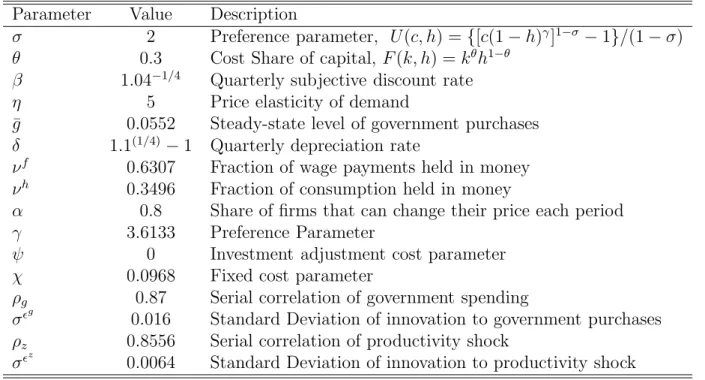
Table 1: Deep Structural Parameters Parameter Value Description
σ 2 Preference parameter, U(c, h) ={[c(1−h)γ]1−σ −1}/(1−σ)
θ 0.3 Cost Share of capital, F(k, h) =kθh1−θ β 1.04−1/4 Quarterly subjective discount rate
η 5 Price elasticity of demand
¯
g 0.0552 Steady-state level of government purchases δ 1.1(1/4)−1 Quarterly depreciation rate
νf 0.6307 Fraction of wage payments held in money νh 0.3496 Fraction of consumption held in money
α 0.8 Share of firms that can change their price each period
γ 3.6133 Preference Parameter
ψ 0 Investment adjustment cost parameter
χ 0.0968 Fixed cost parameter
ρg 0.87 Serial correlation of government spending
σg
0.016 Standard Deviation of innovation to government purchases ρz 0.8556 Serial correlation of productivity shock
σz 0.0064 Standard Deviation of innovation to productivity shock
as we do in this paper (see, for example, Altig et al., 2005). We set the preference parameter γ so that in the deterministic steady state of the competitive equilibrium households allocate on average 20 percent of their time to work, as is the case in the U.S. economy according to Prescott (1986).
The driving forces gt and zt are parameterized as in Schmitt-Groh´e and Uribe (2006).
Government purchases are assumed to follow a univariate autoregressive process of the form
ln(gt/g¯) =ρgln(gt−1/g¯) +
g t,
where ¯g is a constant. The first-order autocorrelation, ρg, is set to 0.87 and the standard
deviation of gt to 0.016. Productivity shocks are also assumed to follow a univariate autore-gressive process
lnzt =ρzlnzt−1+zt,
where ρz = 0.856 and the standard deviation of zt is 0.0064. Finally, we set the fixed
cost parameter χ to ensure zero profits in the deterministic steady state of the competitive equilibrium. Table 1 presents the deep structural parameter values implied by our calibration strategy.
3.2
Measuring Welfare Costs
We conduct policy evaluations by computing the welfare cost of a particular monetary and fiscal regime relative to the time-invariant equilibrium process associated with the Ramsey policy. Consider the Ramsey policy, denoted by r, and an alternative policy regime, denoted by a. We define the welfare associated with the time-invariant equilibrium implied by the Ramsey policy conditional on a particular state of the economy in period 0 as
V0r =E0 ∞ X t=0 βtU(crt, hrt), where cr t and h r
t denote the contingent plans for consumption and hours under the Ramsey
policy. Similarly, define the conditional welfare associated with policy regime a as
V0a=E0
∞
X
t=0
βtU(cat, hat).
We assume that at time zero all state variables of the economy equal their respective Ramsey-steady-state values. Because the non-stochastic steady state is the same across all policy regimes we consider, computing expected welfare conditional on the initial state being the nonstochastic steady state ensures that the economy begins from the same initial point under all possible polices.7
Let λc denote the welfare cost of adopting policy regime a instead of the Ramsey policy
conditional on a particular state in period zero. We define λc as the fraction of regime r’s
consumption process that a household would be willing to give up to be as well off under regime a as under regime r. Formally, λc is implicitly defined by
V0a =E0 ∞ X t=0 βtU((1−λc)crt, h r t).
For the particular functional form for the period utility function given in equation (36), the
7It is of interest to investigate the robustness of our results with respect to alternative initial conditions.
For, in principle, the welfare ranking of the alternative polices will depend upon the assumed value for (or distribution of) the initial state vector. In an earlier version of this paper (Schmitt-Groh´e and Uribe, 2004c), we conduct policy evaluations conditional on an initial state different from the Ramsey steady state and obtain similar results to those presented in this paper.
above expression can be written as V0a = E0 ∞ X t=0 βtU((1−λc)crt, hrt) = (1−λc)1−σV0r+(1−λ c)1−σ −1 (1−σ)(1−β).
Solving for λc we obtain
λc= " 1− (1−σ)V0a+ (1−β) −1 (1−σ)Vr 0 + (1−β)−1 1/(1−σ)# .
Given that we compute Va
0 and V
r
0 accurately up to second-order, we restrict attention to an approximation of λc that is accurate up to second order and omits all terms of order
higher than two. In equilibrium, Va
0 and V0r are functions of the initial state vector x0 and the parameter σ scaling the standard deviation of the exogenous shocks (see Schmitt-Groh´e
and Uribe, 2004a). Therefore, we can write V0a=V
ac
(x0, σ) andV0r=V
rc
(x0, σ). And the
conditional welfare cost can be expressed as
λc= " 1− (1−σ)Vac(x 0, σ) + (1−β)−1 (1−σ)Vrc(x 0, σ) + (1−β)−1 1/(1−σ)# . (37)
It is clear from this expression that λc is a function of x
0 and σ, which we write as
λc = Λc(x0, σ).
Consider a second-order approximation of the function Λc around the point x
0 = x and σ = 0, where xdenotes the deterministic Ramsey steady state of the state vector. Because
we wish to characterize welfare conditional upon the initial state being the deterministic Ramsey steady state, in performing the second-order expansion of Λc only its first and second derivatives with respect to σ have to be considered. Formally, we have
λc≈Λc(x,0) + Λcσ(x,0)σ+
Λcσσ(x,0)
2 σ
2
.
Because the deterministic steady-state level of welfare is the same across all monetary policies belonging to the class defined in equation (17), it follows that λc vanishes at the point
(x0, σ) = (x,0). Formally,
Totally differentiating equation (37) with respect to σ, evaluating the result at (x0, σ) =
(x,0), and using the result derived in Schmitt-Groh´e and Uribe (2004a) that the first derivatives of the policy functions with respect to σ evaluated at (x0, σ) = (x,0) are nil
(Vac σ =V
rc
σ = 0), it follows immediately that
Λcσ(x,0) = 0.
Now totally differentiating (37) twice with respect toσand evaluating the result at (x0, σ) =
(x,0) yields Λcσσ(x,0) = Vrc σσ(x,0)−V ac σσ(x,0) (1−σ)Vrc(x,0) + (1−β)−1. Thus, the conditional welfare cost measure is given by
λc ≈ V rc σσ(x,0)−V ac σσ(x,0) (1−σ)Vrc(x,0) + (1−β)−1 σ2 2 . (38)
Similarly, one can derive an unconditional welfare cost measure, which we denote by λu.
It can be shown that up to second order λu is given by
λu ≈ V ru σσ(0)−V au σσ(0) (1−σ)Vru(0) + (1−β)−1 σ2 2 , (39)
whereVau(σ) andVru(σ) denote the unconditional expectation ofVtaand V r
t , respectively.
4
A Cashless Economy
Consider a nonmonetary economy. Specifically, eliminate the cash-in-advance constraints on households and firms by setting
νh =νf = 0
in equations (5) and (19). The fiscal authority is assumed to have access to lump-sum taxes and to follow a passive fiscal policy. That is, the fiscal policy rule is given by equations (15) and (16) with
γ1 ∈(0,2/π∗) and τtD = 0.
This economy is of interest for it most resembles the canonical neokeynesian model studied in the related literature on optimal policy (see Clarida, Gal´ı, and Gertler, 1999, and the references cited therein). This body of work studies optimal monetary policy in the context of a cashless economy with nominal rigidities and no fiscal authority. For analytical purposes, the absence of a fiscal authority is equivalent to modeling a government that operates under
passive fiscal policy and collects all of its revenue via lump-sum taxation. We wish to highlight, however, two important differences between the economy studied here and the one typically considered in the related literature. Namely, in our economy there is capital accumulation and no subsidy to factor inputs aimed at offsetting the distortions arising from monopolistic competition. The latter difference is of consequence for the solution method that can be applied to the optimal policy problem. Without the ad-hoc subsidy scheme, first-order approximations to the policy functions are not sufficient to deliver a second-order accurate approximation to the utility function. One must approximate the policy functions up to second order to obtain a second-order accurate approximation to the level of welfare. Panel A of table 2 reports policy evaluations for the cashless economy. The point of comparison for our policy evaluation is the time-invariant stochastic real allocation associated with the Ramsey policy. The table reports conditional and unconditional welfare costs, λc
andλu, as defined in equations (38) and (39). Under the Ramsey policy inflation is virtually
equal to zero at all times.8 One may wonder why in an economy featuring sticky prices as the single nominal friction, the volatility of inflation is not exactly equal to zero at all times under the Ramsey policy. The reason is that we do not follow the standard practice of subsidizing factor inputs to eliminate the distortion introduced by monopolistic competition in product markets. Introducing such a subsidy would result in a constant Ramsey-optimal rate of inflation equal to zero.9
We consider seven different monetary policies: Four constrained optimal interest-rate feedback rules and three non-optimized rules. In the constrained optimal rule labeled no-smoothing, we search over the policy coefficients απ and αy keeping αR fixed at zero. The
second constrained-optimal rule, labeled smoothing in the table, allows for interest-rate inertia by setting optimally all three coefficients, απ,αy and αR.
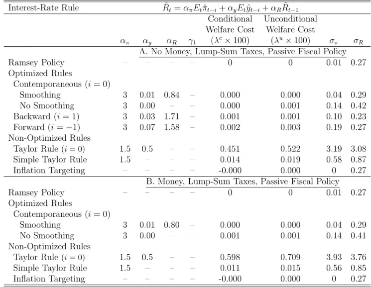
We find that the best no-smoothing interest-rate rule calls for an aggressive response to inflation and a mute response to output. The inflation coefficient of the optimized rule takes the largest value allowed in our search, namely 3.10 The optimized rule is quite effective as it delivers welfare levels remarkably close to those achieved under the Ramsey policy. At the same time, the rule induces a stable rate of inflation, a feature that also characterizes the
8In the deterministic steady state of the Ramsey economy, the inflation rate is zero. 9Formally, one can show that setting τD
t = 1/(1−η) and πt = 1 for all t ≥ 0 and eliminating the
depreciation allowance the equilibrium conditions collapse to those associated with the flexible-price, perfect-competition version of the model. Because the real allocation implied by the latter model is Pareto efficient, it follows that settingπt = 1 at all times must be Ramsey-optimal in the economy with sticky prices and
factor subsidies.
10Removing the upper bound on policy parameters optimal policy calls for a much larger inflation
coeffi-cient, a zero output coefficient and yields a negligible improvement in welfare. The unconstrained policy-rule coefficients areαπ = 332 andαy= 0. The associated welfare gain is about one thousandth of one percent of
Table 2: Optimal Monetary Policy
Interest-Rate Rule Rˆt =απEtπˆt−i+αyEtyˆt−i+αRRˆt−1 Conditional Unconditional Welfare Cost Welfare Cost
απ αy αR γ1 (λc×100) (λu×100) σπ σR
A. No Money, Lump-Sum Taxes, Passive Fiscal Policy
Ramsey Policy – – – – 0 0 0.01 0.27 Optimized Rules Contemporaneous (i= 0) Smoothing 3 0.01 0.84 – 0.000 0.000 0.04 0.29 No Smoothing 3 0.00 – – 0.000 0.001 0.14 0.42 Backward (i= 1) 3 0.03 1.71 – 0.001 0.001 0.10 0.23 Forward (i=−1) 3 0.07 1.58 – 0.002 0.003 0.19 0.27 Non-Optimized Rules Taylor Rule (i= 0) 1.5 0.5 – – 0.451 0.522 3.19 3.08
Simple Taylor Rule 1.5 – – – 0.014 0.019 0.58 0.87
Inflation Targeting – – – – -0.000 0.000 0 0.27
B. Money, Lump-Sum Taxes, Passive Fiscal Policy
Ramsey Policy – – – – 0 0 0.01 0.27 Optimized Rules Contemporaneous (i= 0) Smoothing 3 0.01 0.80 – 0.000 0.000 0.04 0.29 No Smoothing 3 0.00 – – 0.001 0.001 0.14 0.41 Non-Optimized Rules Taylor Rule (i= 0) 1.5 0.5 – – 0.598 0.709 3.93 3.76
Simple Taylor Rule 1.5 – – – 0.011 0.015 0.56 0.85
Inflation Targeting – – – – -0.000 0.000 0 0.27
Notes: (1) In the optimized rules, the policy parametersαπ, αy, andαR are restricted
to lie in the interval [0,3]. (2) Conditional and unconditional welfare costs,λc×100 and
λu×100, are defined as the percentage decrease in the Ramsey optimal consumption process necessary to make the level of welfare under the Ramsey policy identical to that under the evaluated policy. Thus, a positive figure indicates that welfare is higher under the Ramsey policy than under the alternative policy. (3) The standard deviation of inflation and the nominal interest rate is measured in percent per year.
Ramsey policy.
We next study a case in which the central bank can smooth interest rates over time. Our numerical search yields that the optimal policy coefficients are απ = 3, αy = 0.01, and
αR= 0.84. The fact that the optimized rule features substantial interest-rate inertia means
that the monetary authority reacts to inflation much more aggressively in the long run than in the short run. The fact that the interest rule is not superinertial (i.e.,αR does not exceed
unity) means that the monetary authority is backward looking. So, again, as in the case without smoothing optimal policy calls for a large response to inflation deviations in order to stabilize the inflation rate and for no response to deviations of output from the steady state. The welfare gain of allowing for interest-rate smoothing is insignificant. Taking the difference between the welfare costs associated with the optimized rules with and without interest-rate smoothing reveals that agents would be willing to give up less than 0.001 percent, that is,less than 1 one-thousandth of one percent, of their consumption stream under the optimized rule with smoothing to be as well off as under the optimized policy without smoothing.
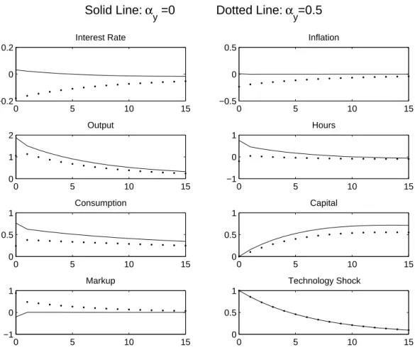
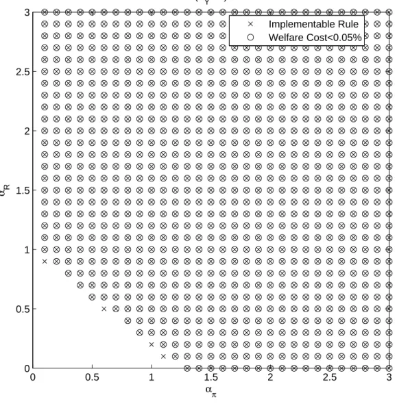
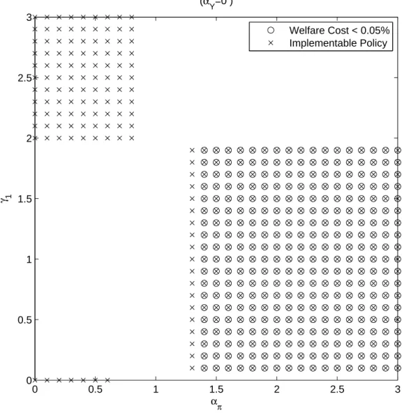
The finding that allowing for optimal smoothing yields only negligible welfare gains spurs us to investigate whether rules featuring suboptimal degrees of inertia or responsiveness to inflation can produce nonnegligible welfare losses at all. Figure 1 shows that provided the central bank does not respond to output, αy = 0, varying απ and αR between 0 and 3
typically leads to economically negligible welfare losses of less than five one-hundredths of one percent of consumption. The graph shows with crosses combinations of απ and αR
that are implementable and with circles combinations that are implementable and that yield welfare costs less than 0.05 percent of consumption relative to the Ramsey policy.
The blank area in the figure identifiesαπ andαRcombinations that are not implementable
either because the equilibrium fails to be locally unique or because the implied volatility of interest rates is too high. This is the case for values ofαπ andαRsuch that the policy stance is
passive in the long run, that is απ
1−αR <1. For these parameter combinations the equilibrium
is not locally unique. This finding is a generalization of the result, that when the inflation coefficient is less than unity (απ < 1) the equilibrium is indeterminate, which obtains in
the absence of interest-rate smoothing (αR = 0). We also note that the result that passive
interest-rate rules (together with passive fiscal policy) renders the equilibrium indeterminate is typically derived in the context of models that abstract from capital accumulation. It is therefore reassuring that this particular abstraction appears to be of no consequence for the finding that (long-run) passive policy is inconsistent with local uniqueness of the rational expectations equilibrium. Similarly, we find that determinacy obtains for policies that are active in the long run, απ
1−αR >1.
Figure 1: Implementability and Welfare in the Cashless Economy 0 0.5 1 1.5 2 2.5 3 0 0.5 1 1.5 2 2.5 3 απ α R (αY=0 ) Implementable Rule Welfare Cost<0.05%
Note: A cross indicates that the policy parameter combination is implementable. A circle indicates that the parameter combination is implementable and that the associ-ated (unconditional) welfare cost is less than 0.05 percent of the Ramsey consumption stream.
feedback rule that are implementable yield virtually the same level of welfare as the Ramsey equilibrium. This finding suggests a simple policy prescription, namely, that any policy parameter combination that is irresponsive to output and active in the long run is equally desirable from a welfare point of view.
One possible reaction to the finding that implementability-preserving variations in απ
and αR have little welfare consequences may be that in the class of models we consider
welfare is flat in a large neighborhood around the optimum parameter configuration, so that it does not really matter what the government does. This turns out not to be the case in the economy studied here. Recall that in the welfare calculations underlying figure 1 the response coefficient on output, αy, was kept constant and equal to zero. Indeed, as we show
in the next subsection, interest-rate policy rules that lean against the wind by raising the nominal interest rate when output is above trend can be associated with sizable welfare costs.
4.1
The importance of not responding to output
Figure 2 illustrates the consequences of introducing a cyclical component to the interest-rate rule. It shows that the welfare costs of varying αy can be large, thereby underlining the
importance of not responding to output. The figure shows the welfare cost of deviating from the optimal output coefficient (αy ≈ 0) while keeping the remaining two coefficients
of the interest-rate rule at their optimal values (απ = 3 and αR = 0.84). Welfare costs are
monotonically increasing in αy. When αy = 1, the welfare cost is over two tenths of one
percent of the consumption stream associated with the Ramsey policy. This is a significant figure in the realm of policy evaluation at business-cycle frequency. This finding suggest that bad policy can have significant welfare costs in our model and that policy mistakes are committed when policy makers are unable to resist the temptation to respond to output fluctuations.
It follows that sound monetary policy calls for sticking to the basics of responding to in-flation alone.11 This point is conveyed with remarkable simplicity by comparing the welfare consequences of a simple interest-rate rule that responds only to inflation with a coefficient of 1.5 to those of a standard Taylor rule that responds to inflation as well as output with coefficients 1.5 and 0.5, respectively. Panel A of table 2 shows that the Taylor rule that responds to output is significantly welfare inferior to the simple interest-rate rule that re-sponds solely to inflation. Specifically, the welfare cost of responding to output is about half a percentage point of consumption.12
11Other authors have also argued that countercyclical interest-rate policy may be undesirable (e.g., Ireland,
1996; and Rotemberg and Woodford, 1997).
Figure 2: The Importance of Not Responding to Output: The Cashless Economy 0 0.1 0.2 0.3 0.4 0.5 0.6 0.7 0 0.05 0.1 0.15 0.2 0.25 αy welfare cost ( λ u × 100)
Note: The welfare cost is measured unconditionally relative to the Ramsey policy and is given by λu×100. See equation (39).