Vahid RahdariA, Alireza SoffianianA*, Saeid PourmanafiA, Razieh MosadeghiB,Hamid Ghaiumi MohammadiC
Received: August 22, 2017 | Revised: October 6, 2017 | Accepted: November 27, 2017 DOI: 10.5937/22-16620
A Hierarchical Approach
of Hybrid Image Classification for Land use
and Land cover Mapping
A Natural Resource Faculty, University of Zabol, Iran, [email protected]; [email protected]; [email protected] B Griffith Centre for Coastal Management, Griffith University, QLD, Australia, [email protected]
C Soil & Geomorphology in Iranian Soil and Water Research Institute, Isfahan, Iran, [email protected] * Corresponding author: Alireza Soffianian, e-mail: [email protected]
Abstract
Remote sensing data analysis can provide thematic maps describing land-use and land-cover (LULC) in a short period. Using proper image classification method in an area, is important to overcome the pos-sible limitations of satellite imageries for producing land-use and land-cover maps. In the present study, a hierarchical hybrid image classification method was used to produce LULC maps using Landsat The-matic mapper TM for the year of 1998 and operational land imager OLI for the year of 2016. Images were classified using the proposed hybrid image classification method, vegetation cover crown percent-age map from normalized difference vegetation index, Fisher supervised classification and object-based image classification methods. Accuracy assessment results showed that the hybrid classification meth-od prmeth-oduced maps with total accuracy up to 84 percent with kappa statistic value 0.81. Results of this study showed that the proposed classification method worked better with OLI sensor than with TM. Al-though OLI has a higher radiometric resolution than TM, the produced LULC map using TM is almost accurate like OLI, which is because of LULC definitions and image classification methods used. Keywords: Error matrix, Hierarchical classification, Iran, land use/cover, Plasjan sub-basin
Introduction
Satellite data are often used to prepare land-use and land-cover maps. (Chrysoulakis et al., 2010; Lakshmi et al., 2015). Selection of proper land-use classification method is crucial in many inventories especially in wa-tershed’s uplands, which are usually water sources for wetlands (Anderson, 1976; Purkis et al., 2006; Mie et al., 2015; Tian et al., 2015). When satellite images data are used to produce LULC map, it is often very difficult to identify spectrally unique land-use/cover classes be-cause of similar spectral responses arising from differ-ent features (Roy et al., 2014; Knudbya et al., 2014;
Es-toque & Murayama, 2015; Lakshmi et al., 2015). Several methods can be employed to produce LULC by em-ploying remote sensing data (Purkis & Klemas, 2011; Lakshmi et al., 2015; Al-doski et al., 2013). However, it should be noted that in case land surface objects have a similar reflectance or a small area, most of them could not provide high accurate maps (Gao & Xu, 2016). Us-ing low radiometric resolution imageries, land classi-fication can be a serious challenge because of spectral mixing of different surface elements and landscape complexity (Julien et al., 2011; Stenzel et al., 2016).
In such cases, application of hybrid classifica-tion approach in hierarchical way will produce bet-ter land-use/land-cover maps (Lakshmi et al., 2015). In this method, land-use/land-cover maps are produced by combining different methods like unsupervised, supervised, object-based methods and different indi-ces produced from satellite images (Anderson, 1976; Homer et al., 2004; Di Gregorio, 2005; Disperati et al., 2015; Misra & Balaji, 2015; Lakshmi et al., 2015).
Several studies compared the accuracies obtained by different image classification methods and
ap-plied imageries with different radiometric resolu-tionsfor producing accurate LULC maps (Benfield et al., 2007; Alves et al, 2012; Vieira et al., 2012; Al-dos-ki et al., 2013; Knudbya et al., 2014; Estoque & Mu-rayama, 2015; Mei et al., 2015; Disperati et al., 2015; Poursanidis et al., 2015; Mirsa & Balaji, 2015; Knud-by et al., 2015 ).
The objective of this study is to develop a hybrid classification method to prepare accurate land-use/ cover maps even when imageries with lower radio-metric resolutions are used.
Methods and data
The study area
The study area was Pelasjan sub-basin including the western part of the Gavkhooni watershed located in central Iran and covering approximately 412,999 hec-tares. The Zayandehrood is the major river in Gavk-hooni watershed to which Pelasjan sub-basin gives the highest portion of water. The Gavkhooni wetland is located in the eastern part of Gavkhooni watershed and is the terminal basin of the Zayandehrood River. Pelasjan sub-basin average temperature is 8-13 Cº with 400-1250 mm precipitation. Agriculture activities and animal husbandry are the main activities of people living in these areas. Figure 1 shows the location of the Zayanderood River Basin and Pelasjan sub-basin in the western part of the Gavkhooni wetland in Iran.
Dataset
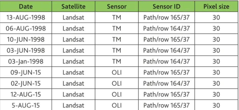
The Operational Land Imager (OLI) and Themat-ic Mapper (TM) sensors were launched with Land-sat Land-satellites and are useful in natural resources stud-ies. OLI sensor measures in the visible, near infrared, and short wave infrared portions of the spectrum in 11 bands. TM sensors with 7 bands are in visible wave-lengths and in infrared. The temporal resolution of both TM and OLI are 16 days. Considering the fact that the study area was located between two Landsat paths, 164 and 165, two images were downloaded from the USGS website. Because thehighest vegetation cover was in June and August, satellite images were downloaded for susceptive months. Table 1 shows sat-ellite data selected for this study.
In addition, aerial images, digital elevation model 1:25/000 topographic maps were used to best
under-stand the study area’s situation. Field studies
Field studies were conducted to collect training areas for each LULC class to be used in the image classifi-cation. Positions of the lands under agricultural areas were determined with GPS. To check the status of the vegetation cover crown percentage (VCCP), 270 plots with 7∙3 meters were measured.
In this study, samples from each LULC were col-lected by paying attention to imageries spatial resolu-tion (30m); and they were collected in a homogenous area of LULC. In this order, we take samples in ho-mogenous areas, which at least are more than 30-me-tersdistant from margins. Therefore, by avoiding mar-ginal land-use/land-cover reflectance, we achieve almost pure reflectance samples for each LULC.
Because there were not enough data for 1998 im-age, by using topographic maps and aerials and by comparing TM and OLI image false color composites (FCC), NDVI images values in TM and OLI and field studies, VCCP in each recorded plot was predicted. LULC classification
Based on the available data and field studies, 7 LULC classes were defined for the study area (Table 2).
Satellite image Pre-processing
Earth atmosphere is a mixed of gases, liquid and sol-id particles, most of these are optically active causing absorption, diffusion and scattering. Signals which measured at the satellite is the emergent radiation from the earth surface atmosphere system in the se-nor observation direction. The radiance measured at sensor is known as Top of Atmosphere (TOA) ra-diance. Atmospheric corrections aim to convert the TOA radiance of the objects into the near earth reflec-tance (Lakshmi et al., 2015). Atmospheric correction was done using Fast Line-of-sight Atmospheric Anal-ysis of Spectral Hypercubus (FLAASH) algorithm. FLAASH was developed to provide accurate, physics-based derivation of atmospheric properties in Envi 5.1. FLAASH includes correction for the adjacency effect, cirrus and opaque cloud classification and adjustable spectral polishing for artifact suppression (Jia et al, 2014; Lakshmi et al., 2015).
Satellite image processing – Hierarchical image classification
First, for image processing, the conceptual model of the three-level earth’s surface matrix that was shown in Figure 2 was applied on both TM and OLI data.
Table1. Satellite sensor specification
Date Satellite Sensor Sensor ID Pixel size
13-AUG-1998 Landsat TM Path/row 165/37 30
06-AUG-1998 Landsat TM Path/row 164/37 30
10-JUN-1998 Landsat TM Path/row 165/37 30
03-JUN-1998 Landsat TM Path/row 164/37 30
03-Jan-1998 Landsat TM Path/row 164/37 30
09-JUN-15 Landsat OLI Path/row 165/37 30
02-JUN-15 Landsat OLI Path/row 164/37 30
12-AUG-15 Landsat OLI Path/row 165/37 30
5-AUG-15 Landsat OLI Path/row 165/37 30
Table 2. LULC classification (Feranec, et al., 2007; Feranec, et al., 2010)
Short description Class
Agricultural arewhich mainly are drainage with other than
rain water Drainage agriculture
Agriculture areas that irrigate only with rain water Rain-fed agriculture Natural vegetation upper than 50% Dense range land Vegetation cover crown less than 50% Sparse range land
Trees with rangelands Forest
Housing developments Residential areas
First step
At this step, the lower cover crown percentage of rain-fed agriculture was considered as the threshold of 50% cover crown for separating from sparse rangeland and other LULC. To map VCCP, NDVI index was used as follows (Equation 1) (Mukherjee, 2004; Oldeland et al., 2010; Peña & Brenning, 2015):
= −
+ NDVI NIRb REDb
NIRb REDb
Simple linear regression was done between sam-ples taken as the dependent variables and their NDVI values for each image as independent variables. Us-ing prepared VCCP models, the VCCP maps prepared two classes of dense vegetation and sparse vegetation. Field control and comparison with FCC image showed that there were some mixings between the cultivation area (especially rain fed agriculture) and dense range-land. In this step, because of drainage, agriculture ar-eas separate more correctly.
Second step
For initial separation of the rain-fed agricultural area and dense rangeland during field studies, and by over-laying first step vegetation map on slope percentage image, it become clear that 30 percent slope was the threshold between rain-fed area and dense range-land. On the other hand, there was no rain-fed cul-tivation over 30 percent slope in mountain areas. By applying 30 percent slope threshold in the first step, dense vegetation in more than 30 percent, which were mostly dense rangelands and forests, were separated from dense vegetation in less than 30 percent slope
that were mostly drainage and rain-fed agricultural areas (Figure 2).
Third level
On the third level of the hierarchical model (Figure 2), four categories: drainage, rain-fed agriculture, forest and dense rangeland were considered as the sub-class-es for the dense vegetation (>50% vegetation coverage). On the other hand, three categories were determined as the sub-classes for the low-density vegetation (<50%) including residential areas, sparse rangeland, and land under water. Because agriculture lands have geomatics shapes, by paying attention to their reflec-tance and their shape, they were classified as rain-fed and drainage agriculture using object-based image classification method, and were separated from satel-lite data. Other LULCs were classified with Fisher su-pervised image classification. Residential area maps for TM image were produced using TM image for January1998 when the land was totally covered with snow, only residential areas did not have snow cover; and residential areas were separated by applying Fish-er image classification method.
Finally, all the individual layers were combined to produce LULCs maps.
Maps accuracy assessment
For accuracy assessment, samples were collected in field studies and were used for TM images. Some areas were selected as samples by considering field studies results and FCC images comparison. The overall ac-curacy and Kappa coefficient, commission error and omission were also determined.
Figure2. Hierarchical structure of Pelasjan matrix Dense
range land bodiesWater Waterbody
Dense vegetation area
Forest and
range land range landDense agricultureDrainage agricultureRain feed Upper than
30% slope 30% slopeLowerthan
Sparse vegetation area
Sparse
range land range landSparse Water
body Residentialarea
Upper than
30% slope 30% slopeLowerthan
Fir st step Second step Th ird step Study area
Results and discussion
Satellite image classification
In supervised classification methods, especially in Fisher classification method, to produce accurate maps, it is important to take samples that are really pure samples of each land-use reflectance (Al-doski et al., 2013). Therefore, samples for each land-use must be prepared in areas far from margins of a land-use/ land-cover. In this study, by proposing a sampling in heterogeneous area of each land-use/land-cover and by taking at least 30 meters distance from margin-al land-use/land-cover (pixels in border of two land uses/land covers), we managed to achieve pure sam-ples that were really samsam-ples of a land use/land-cov-er (LULC).
Image classifications results have shown that LULC classes with similar reflectance values in different bands have more errors. Moreover, small patches of isolated land covers can increase the classification er-rors because of impacts of the reflections from the adjacent pixels. In their studies, Luna, Cesar (2003); Yuan et al.(2005); Kamusoko and Aniya (2007); Lak-shmi et al. (2015); Estoque and Murayama (2015), men-tioned that similarity between LULCs increase errors in image classification. Kamusoko and Aniya (2007) explained that the accuracy of the classification de-pends on the degree of differentiation among the spectral reflections of LULC classes. Figures 3a and 3b
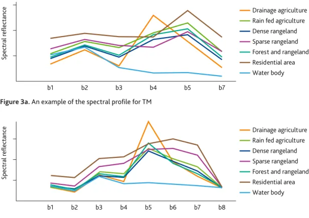
show graphs signatures over used bands for TM and OLI simultaneously either as a spectral response pat-tern or mean reflectance (b1…n= band number).
As shown in figures 3a and 3b, especially the dense rangeland and rain-fed agriculture follow almost sim-ilar reflectance patterns in all bands of the imageries. In these images, rain-fed, dense rangeland and forest almost have the same reflectance trend. Residential areas have high reflectance in all bands, and water re-flectance is the lowest after near infrared band.
In this study, by paying attention to LULC simi-larity and complexity, hierarchical scheme of LULC was designed for satellite image classification. Dis-perati et al. (2015), for satellite image classification, de-signed 3 and 4 levels for land classes and mentioned they produced land maps in each level; and at the end, they combined all results together to achieve the final LULC map.
In this study, for VCCP, models were prepared us-ing NDVI index that is a common and useful vege-tation index for surviving different kinds of plants (Mukherjee, 2004; Oldeland et al., 2010; Jovanović et al., 2015). Formulae 2 and 3 have shown the vegetation cover crown percentage model.
Equivalent 2:
Y = 179.3X + 24.89
R² = 0.89 P-value < 0.01 for the year 2016
(1)
Figure 3a. An example of the spectral profile for TM
Figure 3b. An example of the spectral profile for OLI
Spectr
al r
eflectance
b1 b2 b3 b4 b5 b7
Drainage agriculture Rain fed agriculture Dense rangeland Sparse rangeland Forest and rangeland Residential area Water body Spectr al r eflectance b1 b2 b3 b4 b5 b6 b7 b8 Drainage agriculture Rain fed agriculture Dense rangeland Sparse rangeland Forest and rangeland Residential area Water body
Equivalent 3:
Y= 240.95x + 16.13
R² = 0.80 P-value < 0.0 for the year 1998
Where Y is vegetation cover crown percentage, and X is values in NDVI index.
The range of NDVI values are -1 to 1, the lower val-ues show lower VCCP and the upper valval-ues are relat-ed to areas with more VCCP. In this study, initial im-age classifications showed that it was not possible to separate agricultural area especially rain-fed agricul-ture from dense rangeland. In addition, NDVI classi-fication on the basis of produced modes could not sep-arate dense rangeland from agriculture areas in the first level. The field samplings and overlaying FCC im-ages on slope map indicated that dense rangelands are normally located on slopes greater than 30 percent in mountain areas, while drainage and rain-fed agricul-ture were located on slopes less than 30 percent slope. Thus, by overlaying the slope layer on the satellite im-ages in GIS area using multiple method, dense range-lands which were mostly located on mountain areas were separated.
Finally, LULC maps were proposed using the con-ceptual model, and images were classified with hybrid
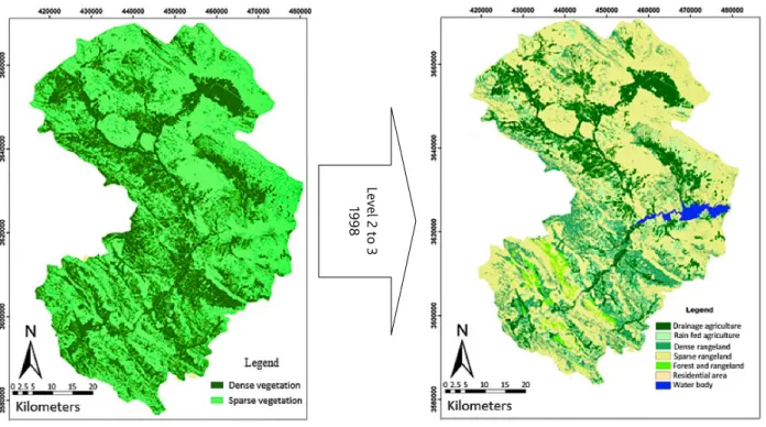
method in 7 layers for years 1998 and 2016. Yuan, et al. (2005); Kamusoko and Aniya (2007) used hybrid image classification and explained that this method is applicable in land with complex reflectance. Fig-ures 4a and b and 5a and b, respectively show LULC maps of the area in the second and third stages. Table 4 shows each class area in hectares.
Residential areas that were small patches were dis-tributed across the study area, and therefore their re-flectance was influenced by the neighboring pix-els (Malmir et al., 2015). Fisher classification method was able to separate the residential areas in both sen-sors. In some cases, residential areas and low-densi-ty rangeland were classified as one class in TM sen-sor images. Fisher supervised classification method can separate LULC with high accuracy when training sites were collected accurately (Al-doski et al., 2013). In this study, samples from each LULC were collected by paying attention to OLI spatial resolution; and they were collected in homogenous areas. Table 4 shows there is no significant change in drainage agriculture area and increase in rain-fed agriculture. From 1998 to 2016, water area in The Zayandehrood dam had a 1671-hectare decrease. On the basis of table 2, during this time, dense rangelands and forests decreased, too.
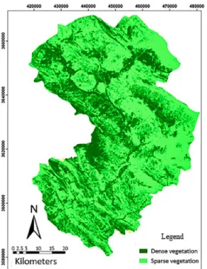
Figure.4a. Dense and sparse vegetation (level 2) Figure.4b. LULC map (level 3)
Level 2 to 3
1998
Table 4. Pelasjan sub-basin LULC area (Hectare) LULC class/
Area (ha) agricultureDrainage agricultureRain-fed range landDense range landSparse Forest Residential area Water body
Class area 1998 58665 18285 58135 257929 12028 3467 4490
Accuracy assessment of classification
In this study, for classification accuracy assessment using field study samples and produced maps, error matrices produced for hybrid method results, and kappa coefficient, overall accuracy, precision of pro-ducer and user, commission and omission errors were
calculated and shown in Tables 5 and 6 (Lunetta & Lyon, 2004; Benfield et al., 2007; Al-doski et al., 2015, Lakshmi et al., 2015).
Error matrices, tables 5 and 6, show that most er-rors related to misclassified areas are related to rain-fed and drainage agriculture areas and dense range
Figure 5a. Dense and sparse vegetation 5(level 2) Figure 5b. 9LULC map (level 3)
Level 2 to 3
2016
Table 5. LULC error matrix for map1998 (Pixel) Classes agricultureDrainage agricultureRain-fed
Dense range land Sparse range land Forest Residential area Water
body Total ErrorC Drainage agriculture 21695 448 1825 21 857 164 0 25037 0.1335 Rain-fed agriculture 1850 3017 1850 511 627 13 0 6069 0.5017 Dense range land 166 539 24564 2114 1947 1 0 29331 0.1625 Sparse range land 408 209 1772 42715 3721 550 0 49375 0.1351 Forest 0 0 1660 454 6973 0 0 7887 0.1159 Residential area 63 0 0 425 0 3636 0 3944 0.1021 Water body 0 0 0 0 0 0 14552 14552 0 Total 24119 4213 31671 46240 14125 4681 14552 136195 -Error0 0.1028 0.2839 0.2244 0.0762 0.5063 0.2232 0 -
-ErrorO = Errors of Omission (expressed as proportions) ErrorC = Errors of Commission (expressed as proportions)
90% Confidence Interval = +/- 0.000815 ( 0.046447 – 0.048076) 95% Confidence Interval = +/- 0.000971 ( 0.046291 – 0.048232) 99% Confidence Interval = +/- 0.001278 ( 0.045984 – 0.048539) Kappa: 0.81
lands together. Figures 3.a and b show that these mis-classifications are related to similarity between drain-age and rain-fed agriculture in dense rangeland areas. TM error matrix (table 5) has shown that most
mis-classifications are for relating rain-fed agriculture to dense rangelands and forests.
Table 6indicates that in the map prepared by OLI image, rain-fed agriculture, drainage agriculture, dense and sparse rangelands were separated correct-ly. In prepared maps, some drainage agricultural pix-els are wrongly related to residential areas because of small green spaces in residential areas. On the other hand, because forests included trees and rangeland
to-gether, in this class, there is a high misclassification be-tween different vegetation classes, and therefore it has high commission and omission error in two imageries.
Using TM and OLI images, land-use/land-cov-er was extracted due to diffland-use/land-cov-erent reflectance behav-iors of water compared to other phenomena (Figure 3 a and b). Tables 5 and 6show produced map using TM sensor has overall accuracy 84% and with kappa coefficient 0.81, and produced map using OLI sensor has overall accuracy 91% and with kappa coefficient 0.87,which is more than TM. This difference was pre-dictable because of OLI characteristics like more radi-ometric and spectral resolution.
Conclusion
LULC spectral profiles have shown LULCs digital numbers were more separated in OLI with 16-bit than TM data, so this is the reason for the less accuracy in TM map with 8-bit radiometric resolution (Figures 3a and 3b). Applying proposed hybrid method inland hi-erarchy concept could produce almost the same accu-rate maps for two imageries data. In this study, Fisher classification (Al-doski et al., 2013), object-based clas-sification (Blaschke, 2010; Vieira et al., 2012; Phinn et al., 2012), and NDVI vegetation index (Peña & Bren-ning, 2015; Oldeland et al., 2010) were used in designed hybrid classification method.
Error matrices have shown more accurate image classification results in the map provided by OLI sen-sor than TM, especially in mapping different vegeta-tion types and separating land surfaces such as resi-dential areas.
Considering the similarity of some LULC reflec-tance in this study, in the hierarchy concept of land matrix, hybrid method can produce acceptable LULC maps. Thus, providing detailed maps of LULC that have small areas and similar reflectance will be pos-sible through appropriate methods for each defined land level using different imageries.
Table 6. LULC error matrix for map 2016 (Pixel) Drainage
agriculture agricultureRain-fed
Dense range land Sparse range land Forest Residential
area Water body Total ErrorC Drainage agriculture 23608 998 463 106 93 95 0 25363 0.0692 Rain-fed agriculture 537 5240 1665 23 19 5 0 7489 0.3003 Dense range land 15 1047 28549 71 1019 0 0 29669 0.0700 Sparse range land 573 15 2758 43088 1336 181 0 48983 0.1203 Forest 0 0 1784 0 13241 0 0 15025 0.1187 Residential area 0 0 0 264 99 3390 0 3753 0.0967 Water body 0 0 0 0 0 0 14552 14552 0 Total 24733 7300 33577 45594 15907 3171 14552 144834 -Error0 0.0454 0.2821 0.1893 0.0106 0.1623 0.0765 0 131668
-ErrorO = Errors of Omission (expressed as proportions) ErrorC = Errors of Commission (expressed as proportions)
90% Confidence Interval = +/- 0.000815 ( 0.046447 – 0.048076) 95% Confidence Interval = +/- 0.000971 ( 0.046291 – 0.048232) 99% Confidence Interval = +/- 0.001278 ( 0.045984 – 0.048539) Kappa: 0.87
References
Al-doski, J., Shattri, M., & Zulhaidi, M.S. (2013). Image classification in remote sensing. Journal of Environ-ment and Earth Science, 3(10), 141-147.
Anderson, J.R. (1976). A Land Use and Land Cover Classification System for Use with Remote Sensor Data. U. S. Government Printing Office.
Benfield, S.L., Guzman, H.M., Mair, J.M., & Young, J.A.T. (2007). Mapping the distribution of coral reefs and associated sublittoral habitats in Pacif-ic Panama: a comparison of optPacif-ical satellite sen-sors and classification methodologies. Internation-al JournInternation-al of Remote Sensing, 28, 5047-5070.
Blaschke, T. (2010). Object based image analysis for remote sensing. ISPRS Journal of Photogrammetry and Remote Sensing, 65, 2-16.
Chrysoulakis, N., Abrams, M., Feidas, H., & Korei, A. (2010). Comparison of methods using ASTER data for the area of Crete, Greece. International Journal of Remote Sensing, 31(24), 6347-6385.
Di Gregorio, A. (2005). Di Gregorio, A. (2005). Land cover classification system: Classification concepts and user manual: LCCS (No. 8). Rome: Food and Agriculture Organization of the United Nations. Disperati, L., Gonario, S., & Virdis, P. (2015).
Assess-ment of land-use and land-cover changes from 1965 to 2014 in Tam Giang-Cau Hai Lagoon, central Vi-etnam. Applied Geography, 58, 48-64.
Estoque, R.C., & Murayama, Y. (2015). Classification and change detection of built-up lands from Land-sat-7 ETM+ and Landsat-8 OLI/TIRS imageries: A comparative assessment of various spectral indi-ces. Ecological Indicators journal, 56, 205-217. Feranec, J., Hazeu, G., Christensen, S., & Jaffrain, G.
(2007). CORINE land cover change detection in Europe (case studies of the Netherlands and Slova-kia). Land Use Policy, 24(1), 234-247.
Feranec, J., Jaffrain, G., Soukup, T., & Hazeu, G. (2010). Determining changes and flows in European land-scapes 1990e2000 using Corine land cover data. Ap-plied Geography, 30(1), 19-35.
Gao, J., & Xu, L. (2016). An efficient method to solve the classification problem for remote sensing im-age. AEU - International Journal of Electronics and Communications, 69(1), 198-205.
Homer, C., Huang, C., Yang, L., Wylie, B., & Coan, M. (2004). Development of a 2001 national land cov-er database for the United States. Photogrammetric Engineering and Remote Sensing, 70(7), 829-840. Jia, K., Wei, X., Gu, X., Yao, Y., Xie, X., & Li, B. (2014).
Land cover classification using land sat 8 operation land imager data in Beijing, China. Geocarto inter-national, 29(8), 941-951.
Jovanović, M., & Milanović, M. (2015). Normalized Difference Vegetation Index (NDVI) as the Basis for Local Forest Management. Example of the Mu-nicipality of Topola, Serbia. Polish Journal of Envi-ronmental Studies, 24(2), 529-535.
Julien, Y., Sobrino, J.A., & Jiménez-Muñoz, (2011). Land use classification from multi-temporal Land-sat imagery using the Yearly Land Cover Dynamics (YLCD) method. International Journal of Applied Earth Observation and Geoinformation, 13, 711-720. Kamusoko, C., & Aniya, M. (2007). Land use/cover
change and landscape fragmentation analysis in the Bindura District, Zimbabwe. Land Degradation and Development, 18(2), 221-233.
Knudby, A., Mtwana, N.L., Palmqvistc, G., Wik-strömc, K., Koliji, A., Lindborgd, R., & GullWik-strömc, M. (2014). Using multiple Landsat scenes in an en-semble classifier reduces classification error in a stable nearshore environment. International Jour-nal of Applied Earth Observation and Geo-informa-tion, 28, 90-101.
Lakshmi, N., Kantakumar, L.N., & Neelamsetti, P. (2015). Multi-temporal land use classification using hybrid approach. The Egyptian Journal of Remote Sensing and Space Sciences, 18(2), 289-295.
Luna, A.R., & Cesar, A.R. (2003). Land use, land cov-er changes and costal lagoon surface reduction as-sociated with urban growth in northwest Mexi-co. Landscape Ecology, 18(2), 159-171.
Lunetta, R.S., & Lyon, J.G. (2004). Remote Sensing and GIS Accuracy Assessment. CRC Press.
Malmir, M., Kheirkhah, Z.M.M., Monavari, S.M., Jozi, S.A., & Sharifi, S. (2015). Urban development change detection based on Multi-Temporal Sat-ellite Images as a fast tracking approach—a case study of Ahwaz County, southwestern Iran. Envi-ronmental monitoring and assessment, 187(3), 108. Mei, A., Ciro, M., Fontinovo, M., Bassani, A.A., &
Pe-tracchini, F. (2015). Landsat 8 vs. Landsat 5: A com-parison based on urban and peri-urban land cover mapping Dimitris.. Journal of African earth sci-ence, 5, 15-24.
Misra, A., & Balaji, R. (2015). A Study on the Shoreline Changes and LAND-use/ Land-cover along the South Gujarat Coastline. Procedia Engineering, 116, 381-389. doi:10.1016/j.proeng.2015.08.311
Mukherjee, S. (2004). Text Book of Environmental Re-mote Sensing. New Delhi: Macmillan India Limited. Nurdin, N., Komatsu, T., Agus, , Akbar, A.M., Djalil,
A.R., & Amri, K. (2015). Multisensor and multitem-poral data from Landsat images to detect damage to coral reefs, small islands in the Spermonde
ar-chipelago, Indonesia. Ocean Science Journal, 50(2), 317-325. doi:10.1007/s12601-015-0029-x
Oldeland, J., Dorigo, W., Lieckfeld, L., Lucieer, A., & Jürgens, N. (2010). Combining vegetation indices, constrained ordination and fuzzy classification for mapping semi-natural vegetation units from hy-perspectral imagery. Remote Sensing of Environ-ment, 114(6), 1155-1166. doi:10.1016/j.rse.2010.01.003 Peña, M.A., & Brenning, A. (2015). Assessing
fruit-tree crop classification from Landsat-8 time series for the Maipo Valley, Chile. Remote Sensing of En-vironment, 171, 234-244. doi:10.1016/j.rse.2015.10.029 Phinn, S.R., Roelfsema, C.M., & Mumby, P.J. (2012).
Multi-scale, object-based image analysis for map-ping geomorphic and ecological zones on cor-al reefs. International Journal of Remote Sens-ing, 33(12), 3768-3797. doi:10.1080/01431161.2011.6331 22
Poursanidis, D., Chrysoulakis, N., & Mitraka, Z. (2015). Landsat 8 vs. Landsat 5: A comparison based on urban and peri-urban land cover mapping. In-ternational Journal of Applied Earth Observa-tion and GeoinformaObserva-tion, 35, 259-269. doi:10.1016/j. jag.2014.09.010
Purkis, S., & Klemas, V. (2011). Remote Sensing and Global Environmental Change. West Sussex, UK: Wiley-Blackwell. doi:10.1002/9781118687659
Purkis, S.J., Myint, S.W., & Riegl, B.M. (2006). En-hanced detection of the coral Acropora cervi-cornis from satellite imagery using a textural
oper-ator. Remote Sensing of Environment, 101(1), 82-94. doi:10.1016/j.rse.2005.11.009
Roy, D.P., Wulder, M.A., Loveland, T.R., C.E. Wood-cock, , Allen, R.G., Anderson, M.C., . . . Bind-schadler, R. (2014). Landsat-8: Science and product vision for terrestrial global change research. Remote Sensing of Environment, 145, 154-172. doi:10.1016/j. rse.2014.02.001
Stenzel, S., Fassnacht, F.E., Mack, B., & Schmidtlein, S. (2017). Identification of high nature value grass-land with remote sensing and minimal field data. Ecological Indicators, 74, 28-38. doi:10.1016/j. ecolind.2016.11.005
Tian, B., Zhou, Y., Thom, R.M., Diefenderfer, H.L., & Yuan, Q. (2015). Detecting wetland changes in Shanghai, China using FORMOSAT and Land-sat TM imagery. Journal of Hydrology, 529, 1-10. doi:10.1016/j.jhydrol.2015.07.007
Vieira, M.A., Formaggio, A.R., Rennó, C.D., Atzberg-er, C., Aguiar, D.A., & Mello, M.P. (2012). Object Based Image Analysis and Data Mining applied to a remotely sensed Landsat time-series to map sug-arcane over large areas. Remote Sensing of Environ-ment, 123, 553-562. doi:10.1016/j.rse.2012.04.011 Yuan, F., Sawaya, K.E., Loeffelholz, B.C., & Bauer,
M.E. (2005). Land cover classification and change analysis of the Twin Cities (Minnesota) Metropol-itan Area by multitemporal Landsat remote sens-ing. Remote Sensing of Environment, 98(2-3), 317-328. doi:10.1016/j.rse.2005.08.006