Examples of Computing Power for Zero-Inflated and Overdispersed Count Data

(1)

Methods

Volume 8 | Issue 2

Article 3

11-1-2009

Examples of Computing Power for Zero-Inflated

and Overdispersed Count Data

Suzanne R. Doyle

University of Washington, [email protected]

Follow this and additional works at:

http://digitalcommons.wayne.edu/jmasm

Part of the

Applied Statistics Commons

,

Social and Behavioral Sciences Commons

, and the

Statistical Theory Commons

This Regular Article is brought to you for free and open access by the Open Access Journals at DigitalCommons@WayneState. It has been accepted for inclusion in Journal of Modern Applied Statistical Methods by an authorized administrator of DigitalCommons@WayneState.

Recommended Citation

Doyle, Suzanne R. (2009) "Examples of Computing Power for Zero-Inflated and Overdispersed Count Data,"Journal of Modern Applied Statistical Methods: Vol. 8: Iss. 2, Article 3.

(2)

360 REGULAR ARTICLES

Examples of Computing Power for Zero-Inflated and Overdispersed Count Data

Suzanne R. Doyle

University of Washington

Examples of zero-inflated Poisson and negative binomial regression models were used to demonstrate conditional power estimation, utilizing the method of an expanded data set derived from probability weights based on assumed regression parameter values. SAS code is provided to calculate power for models with a binary or continuous covariate associated with zero-inflation.

Key words: Conditional power, Wald statistic, zero-inflation, over-dispersion, Poisson, negative binomial.

Introduction

Lyles, Lin and Williamson (2007) presented a simple method for estimating conditional power (i.e., power given a pre-specified covariate design matrix) for nominal, count or ordinal outcomes based on a given sample size. Their method requires fitting a regression model to an expanded data set using weights that represent response probabilities, given assumed values of covariate regression parameters. It has the flexibility to handle multiple binary or continuous covariates, requires only standard software and does not involve complex mathematical calculations. To estimate power, the variance-covariance matrix of the fitted model is used to derive a non-central chi square approximation to the distribution of the Wald statistic. This method can also be used to approximate power for the likelihood ratio test.

Lyles, et al. (2007) illustrated the method for a variety of outcome types and covariate patterns, and generated simulated data to demonstrate its accuracy. In addition to the proportional odds model and logistic regression, they included standard Poisson regression with one continuous covariate and negative binomial regression with one binary covariate. Both the

Suzanne R. Doyle is a Biostatistician in the Alcohol and Drug Abuse Institute. Email: [email protected].

Poisson and negative binomial regression models provide a common framework for the analysis of non-negative count data. If the model mean and variance values are the same (equi-dispersion), the one-parameter Poisson distribution can be appropriately used to model such count data. However, when the sample variance exceeds the sample mean (over-dispersion), the negative binomial distribution provides an alternative by using a second parameter for adjusting the variance independently of the mean.

Over-dispersion of count data can also occur when there is an excess proportion of zeros relative to what would be expected with the standard Poisson distribution. In this case, generalizations of the Poisson model, known as zero-inflated Poisson (ZIP) and ZIP(_τ) (Lambert, 1992), are more appropriate when there is an excess proportion of zeros and equi-dispersion of the non-zero count data is present. These models provide a mixture of regression models: a logistic portion that accounts for the probability of a count of zero and a Poisson portion contributing to the frequency of positive counts. The ZIP model permits different covariates and coefficient values between the logistic and Poisson portions of the model. Alternatively, the ZIP(_τ) model is suitable when covariates are the same and the logistic parameters are functionally related to the Poisson parameters.

(3)

361

With the ZIP and ZIP(τ) models, the non-zero counts are assumed to demonstrate equi-dispersion. However, if there is zero-inflation and non-zero counts are over-dispersed in relation to the Poisson distribution, parameter estimates will be biased and an alternative distribution, such as the zero-inflated negative binomial regression models, ZINB or ZINB(_τ), are more appropriate (Greene, 1994). Similar to the zero-inflated Poisson models, ZINB allows for different covariates and ZINB(_τ) permits the same covariates between the logistic portion for zero counts and the negative binomial distribution for non-zero counts.

In this study, the use of an expanded data set and the method of calculating conditional power as presented by Lyles, et al. (2007) is extended to include the ZIP, ZIP(_τ), ZINB and ZINB(_τ) models. Examples allow for the use of a binary or a normally-distributed continuous covariate associated with the zero-inflation. Simulations were conducted to assess the accuracy of calculated power estimates and example SAS software programs (SAS Institute, 2004) are provided.

Methodology Model and Hypothesis Testing

Following directly from Lyles, et al. (2007), the response variable Y for non-continuous count data has J possible values (y1,

y2, … , yJ), a design matrix X, and a regression

model in the form of

log(λi) = β′xi (1)

with an assumed Poisson distribution or negative binomial distribution, where i indexes independent subjects (i = 1, ... , N), xi is a (1 x

q) vector of covariates, and β is a (1 x q) vector of regression coefficients. Under the Poisson or negative binomial regression model, the probabilities can be specified for j = 1, … , J by

ij

w = Pr (Yi= yj|Xi=xi), yj = 0, 1, … , ∞

(2) Interest is in testing the hypothesisH0:Hβ=h0

versusHA:Hβ≠h0, where H is an (h x q)

matrix of full row rank and h0 an (h x 1)

constant vector. The Wald test statistic is W = ( ˆ ₀) [ var( ) ]ˆ ˆ 1( ˆ 0)

−

′ ′ −

− Hβ

Hβ h H β H h (3)

where βˆcontains unrestricted maximum likelihood estimates of β. Under H0, (3) is

asymptotically distributed as central chi square with h degrees of freedom (_χ2_h).

For power calculations, under HA, the

Wald test statistic is asymptotically distributed as non-central

_χ

2_h_{,( )}_η , where the non-centrality parameter _η is defined as

η

= (Hβ−h₀) [ var( ) ]′ H ˆ βˆ H′ −1(Hβ−h₀). (4) Creating an Expanded Data Set and Computing Conditional Power

To estimate the conditional power given assumed values of N, X andβ, an expanded data set is first created by selecting a value of J for the number of possible values of Y with non-negligible probability for any specific xi, such

that 1 1Pr( | ) 1 J J i i i ij i j= w = j= Y = y = ≈   X x (5) for all i. The sum in (5) should be checked for each unique value of xi. A reasonable threshold

for the sum (e.g., > 0.9999) is suggested for sufficient accuracy (Lyles et al., 2007). Second, for each value of i = 1, ... , N, a data matrix with

J rows is created with the weightswij in (2)

being computed with the assumed values of β. This data matrix with J rows is stacked N times vertically from i = 1, ... , N to form an expanded data set with NJ records. The resulting expanded data set can be based on the same number of J

records for each value of i. However, J can vary with i, as long as the condition in (5) is satisfied.

When the expanded data set is correctly created maximum likelihood estimate ˆβ from maximizing the weighted log-likelihood should equal the assumed value of β, and the matrix

ˆ ˆ ( )

var β will accurately reflect variability under the specific model allowing for power

(4)

362

calculations based on the Wald test of (3). For more detailed information and examples concerning model and hypothesis testing and creating an expanded data set with this method, see Lyles, et al. (2007).

Subsequent to fitting the model to the expanded data set, the non-centrality parameter

η in (4) is derived. Power is then calculated as Pr 2 2 ( ) ,1 (x_hη ≥ χ_h −α) (6) where 2 ,1 h

x −αdenotes the 100(1 - α) percentile

of the central _χ2distribution with h degrees of freedom. For testing a single regression coefficient, 2 _ˆ2

k k

η = β σ , where ˆσkis the

associated estimated standard error, with h = 1. Zero-Inflated Poisson and Negative Binomial Models

Following Lambert (1992) for the zero-inflated Poisson (ZIP) regression model and Greene (1994) for the zero-inflated negative binomial (ZINB) regression model, the response

i Y is given by 0 i Y  with probability πi, i

Y Poisson(λi) for the ZIP model

or

i

Y NegBin(λi) for the ZINB model,

with probability 1−πi, i = 1, ... , n for both

models. For these models, the probability of zero counts is given by

Pr (Yi=0) = πi+ −(1 πi

)

e−λi

.

(7)

The probability of non-zero counts for the ZIP model is Pr (Yi= yj|Xi=xi) = (1 ) ! , j i _i i j y e y −λ λ − π (8) and for the ZINB model is

Pr (Yi= yj|Xi=xi) = 1/ 1 1 ( ) ₁ (1 ) 1 1 ( ) ! . j j _i i i i j y y y κ − − Γ κ + κ_λ − π _Γ _+κ _+κ λ λ κ             (9)

for y_j = 1, ... , ∞, where Γ is the gamma function. In contrast to the Poisson model with only one parameter, the negative binomial model has two parameters: _λ (the mean, or shape parameter) and a scale parameter,_κ, both of which are non-negative for zero-inflated models, and not necessarily an integer. Both πi of the

logistic model and λiof the Poisson model or

negative binomial model depend on covariates through canonical link of the generalized linear model

logit(πi) = γ′zi

and

with _{γ = γ γ}( , ,..., )₀ ₁ _γ_r and _{β = β β}( , ,...,₀ ₁ _β_p). Because the covariates that influence _π_i and _λ_i are not necessarily the same, two different sets of covariate vectors, zi=(1, ,...,zi1 zir) and

1

(1, ,..., )

i i ip

x = x x , are allowed in the model.

Interpretation of the γ and β parameters is the same as the interpretation of the parameters from standard logistic and Poisson or negative binomial models, respectively.

If the same covariates influence πi and i

λ , and if πi can be written as a scalar multiple

of λi, such that

logit(πi) = −τβ′xi

and

then the ZIP and ZINB models described in (10) are called ZIP(_τ) or ZINB(_τ) models with an unknown scalar shape parameter τ (Lambert, 1992). When _{τ >}0 zero inflation is less likely, and as _{τ →}0 zero inflation increases. Note that the number of parameters in the ZIP(_τ) and ZINB(_τ) models is reduced, providing a more parsimonious model than the ZIP and ZINB

(5)

363

models, and it may therefore be advantageous to use this model when appropriate.

With the ZIP and ZIP(τ) models, the weights for the expanded data set are calculated as ij w = Pr (Yi= yj|Xi=xi) = ( ) (1 ! ) i i j i i i j y e I y y −λ λ + − π π (12)

and for the ZINB and ZINB(_τ) models, the weights for the expanded data set are

ij w = Pr (Yi= yj|Xi=xi) = 1/ 1 1 ( ) ₁ ( ) ( ) (1 1 1 ( ) ) ! j j i i i i j i i y y I y y κ − − Γ _κ + _κ_λ + − π π +κ +κ Γ κ λ λ             (13) with y_j = 0, 1, ... , _∞, and where I y( )_i is an indicator function taking a value of 1 if the observed response is zero (y_i=0)and a value of 0 if the observed response is positive (y_i>0). Simulating the Negative Binomial Distribution

In simulating the negative binomial distribution, Lyles, et al. (2007) generated independent geometric random variates, under the constraint of only integer values for1/_κ. In contrast, the negative binomial distribution in this study was simulated according to the framework provided by Lord (2006). This algorithm is based on the fact that the negative binomial distribution can be characterized as a Poisson-gamma mixture model (Cameron & Trivedi, 2006), it is consistent with the linear modeling approach used with this method of power calculation and also allows for non-integer values of 1/_κ. To calculate an outcome variable that is distributed as negative binomial, the following steps are taken:

1. Generate a mean value (_λ_i) for observation i from a fixed sample population mean, _λ_i = exp(β′xi)

2. Generate a value (_φ_i) from a gamma distribution with the mean equal to 1 and the parameter _{δ = κ}1/ , φ_i= Γ δ δ( ,1/ )

3. Calculate the mean (_θ_i) for observation i,

i= ×φi i

θ λ

4. Generate a discrete value (y_i) for observation i from a Poisson distribution with a mean θi, yiPoisson( )θi .

5. Repeat steps 1 through 4 N times, where N is the number of observations or sample size.

Examples

Several examples are presented to illustrate the conditional power calculations of the ZIP, ZIP(_τ), ZINB and ZINB(_τ) models with a binary or continuous covariate related to the logistic portion accounting for the zero-inflation. Models were selected to demonstrate the effects of increased zero-inflation and over-dispersion on power estimates. Each model was fit by utilizing a weighted form of the general log-likelihood feature in SAS PROC NLMIXED (SAS Institute, 2004). Simulations under each model and the assumed joint covariate distributions were conducted to assess the accuracy of the power calculations. In situations where a reasonable solution could not be obtained with the generated data, the simulation data set was excluded from consideration and data generation was continued until 1,000 usable data sets were obtained for each model. A viable solution was generally due to non-convergence or extremely large standard errors. In particular, the ZIP(_τ) and ZINB(_τ) models were the most problematic due to obtaining extremely large standard errors and parameter estimates of _τ. In some situations it was obvious that a poor solution resulted, but in other instances it was not as clear that an unsatisfactory solution occurred. To avoid arbitrary decisions on which simulations to exclude, all data sets resulting in a value of _τ outside of the boundaries of a 99% confidence interval (based on assumed regression parameter values) were deleted. A similar decision rule was used for the ZIP and ZINB models, eliminating data sets with values of _γ_i, as

(6)

364

defined in (10) beyond their 99% confidence boundaries. The selection decision to discard data sets from consideration did not depend on the values of the regression parameter of interest to be statistically tested.

Simulation values presented are the average regression coefficient and the average standard error (calculated as the square root of the average error variance) out of the 1,000 generated data sets for the parameter estimates of each model. Simulation-based power was calculated as the proportion of Wald tests found statistically significant at _{α =}.05 out of 1,000 randomly generated data sets under each specific model considered. Appendices A through D provide SAS programming code to evaluate a large sample simulation for distributional characteristics, to construct an expanded data set and to calculate power for models with a binary covariate or a normally-distributed continuous covariate related to the zero-inflation.

To calculate the expanded data set, it was first necessary to choose the initial value of

J for each value of xi. This was done by

generating a large simulated data set (N = 100,000 for each binary or continuous covariate in the model) based on the same parameter values of the model. To ensure that a reasonable threshold for the sum (e.g., > 0.9999) of the weights in (12) and (13) would be obtained, the initial value of J was increased in one unit integer increments until the maximum likelihood estimates for the parameters from maximizing the weighted log-likelihood equaled the assumed parameter values of the regression model. The large simulated data set also provided approximations to the population distributional characteristics of each model (mean, variance, and frequencies of each value of the outcome variable yi) and estimates of the percents of

zero-inflation.

ZIP(τ), ZIP, ZINB(τ) and ZINB Models with a Binary Variable for Zero Inflation

Model A-τ and Model B-τ, where τ = 2 and 1, are ZIP(_τ) and ZIP models, respectively. Model A-τ is defined as

logit(πi) = −τβ0− τβ1x and log(λi) = β β0+ 1x

(14)

where _β₀= 0.6931, _β₁ = -0.3567,τ = 2 and 1, and x is a binary variable with an equal number of cases coded 0 and 1. The regression coefficients were based on the rate ratio. That is, for the binary covariate x, from the rates of the two groups (λ1=2 and λ2=1.4), the regression

coefficients are β0=logλ1 and

2 1

1=log( ) log( )−

β λ λ . With this model, interest is in testingH₀:β₁=0versusHA:β₁≠0. Model B-τ is defined as logit(πi) = γ0+γ1z and log(λi) = β β0+ 1z+β2x (15) where _β₀= 0.6931, _β₁ = -0.3567, _β₂ = -0.3567, 0= −τ 0

γ β , _γ₁_{= −τ}_β₁, τ = 2 and 1, and x and z

are binary covariates with an equal number of cases coded 0 and 1. In this particular example the regression coefficients for the logistic portion of the model (_γ₀ and_γ₁) are both a constant multiple ofτ, although this is not a necessary requirement for the ZIP model. With this model, interest is in assessing H0:β2=0

versusHA:β₂≠0.

The ZINB(τ) and ZINB models consisted of the same parameter estimates as the ZIP(τ) and ZIP models (Model A-τ and Model B-τ described above), but included two values of an extra scale parameter, _{κ =}0.75 and

1.50.

κ = Sample sizes were based on obtaining conditional power estimates of approximately .95 for the regression coefficient tested, withτ = 2 for the ZIP and ZIP(_τ) models, and forτ = 2 and _{κ =}0.75 for the ZINB and ZINB(_τ) models. SAS code to evaluate a large sample simulation for distributional characteristics, to construct an expanded data set and to calculate power, for models with a binary covariate related to the zero-inflation are presented in Appendices A and B, for the Poisson and negative binomial regression models, respectively.

(7)

365

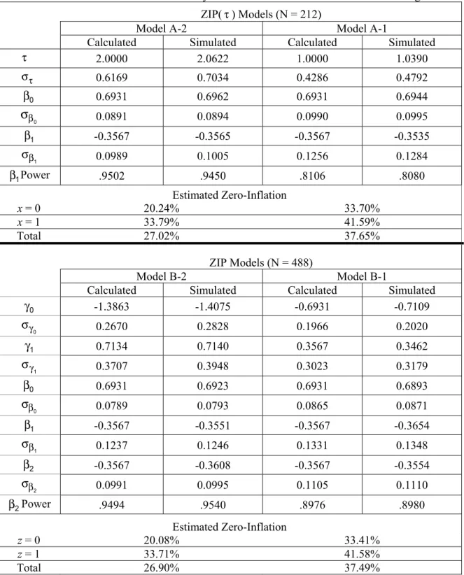
Results ZIP(τ) Models

The results of the ZIP(τ) models presented at the top of Table 1 indicate that with a sample size of N = 212, when _τ = 2, there is approximately .95 power and 27.0% zero-inflation for testing_H_A:β₁≠0. As _τ decreases and therefore zero-inflation increases, the calculated power is reduced to 0.81 for approximately 37.5% estimated zero-inflation. In most cases, the simulated parameter and power estimates match the calculated values, except for a slight tendency for the simulated data to result in inflated average parameter estimates for the standard error

τ σ .

The outcomes for the ZIP models presented at the bottom of Table 1 show that with a sample size of N = 488, when _τ = 2, there is approximately .95 power and 27.0% zero-inflation for testingHA:β₂≠0. Again, as τ decreases, the calculated power is reduced to approximately .90 and 37.5% estimated zero-inflation.

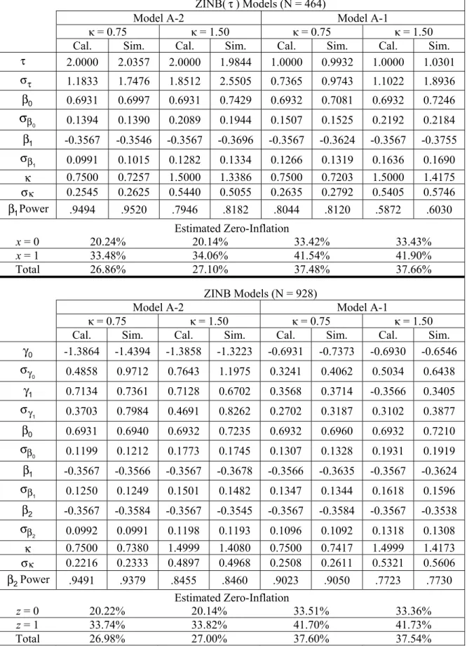
ZINB(_τ) Models With A Binary Covariate Associated With The Zero-Inflation

The results of the ZINB(τ) models with a binary covariate associated with the zero-inflation, presented at the top of Table 2, indicate that with a sample size of N = 464, when_{κ =}0.75 and τ = 2, there is approximately .95 power and 27.0% zero-inflation for testing HA:β₁≠0. As τ decreases

to 1, the calculated power is reduced to approximately .80 and 37.5% estimated zero-inflation. When over-dispersion of the non-zero counts increases (_{κ =}1.50), power is reduced to approximately .80 when τ = 2, and .59 when τ

= 1.

In most cases, the simulated (Sim.) values and power estimates closely match the calculated (Cal.) parameters, except for a slight tendency for the simulated data to result in an inflated average standard error (_σ_τ) associated with parameter estimates for _τ, and slightly lower than expected values for the scale or over-dispersion parameter _κ.

The results of the ZINB models presented at the bottom of Table 2 indicate that with a sample size of N = 928, when _{κ =}0.75 and τ = 2, there is approximately .95 power and 27.0% zero-inflation for testingHA:β₂≠0.

Again, as τ decreases (τ = 1), the calculated power is reduced to approximately .90 with 37.5% estimated zero-inflation. Also, when over-dispersion of the non-zero counts increases (_{κ =}1.50), power is reduced to approximately .85 when _τ = 2, and .77 when _τ = 1. There is also the slight tendency of the simulated data to result in average inflated standard errors (

0 γ σ and 1 γ

σ ) for the parameter estimates of the logistic portion of the model involving zero-inflation (_γ₀ and _γ₁), and in decreased values for the scale or over-dispersion parameter_κthan would be expected.

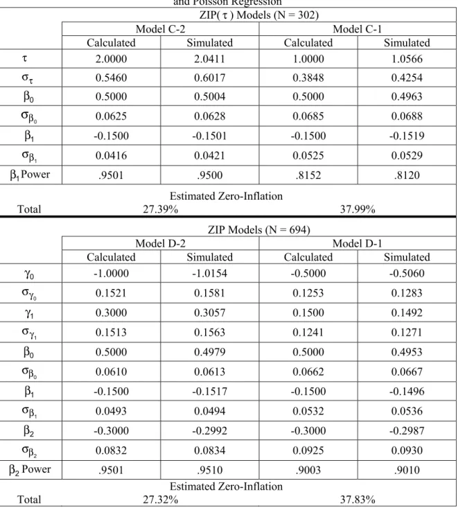
ZIP(_τ), ZIP, ZINB(_τ) and ZINB Models with a Continuous Variable for Zero-Inflation

Model C-τ and Model D-τ, where τ = 2 and 1, are ZIP(_τ) and ZIP models, respectively. Model C-τ is defined as

logit(_π_i) = −τβ₀− τβ₁z and log(_λ_i) = β β₀+ ₁z

(16) where _β₀= 0.5000, _β₁ = -0.1500,τ = 2 and 1, and z is a continuous variable distributed as N(0,1). These are the same parameter estimates of _β₀and _β₁used by Lyles, et al. (2007) with their example of standard Poisson regression with one continuous covariate. With this ZIP(_τ) model, interest is in assessing H0:β1=0 versus

1

: 0

A

H β ≠ . Model D-τ is defined as

logit(πi) = γ0+γ1z and log(λi) = β β0+ 1z+β2x

(17) where _β₀= 0.5000, _β₁ = -0.1500, _β₂ = -0.3000,

0= −τ 0

γ β , γ₁= −τβ₁, τ = 2 and 1, x is abinary variable with an equal number of cases coded 0 and 1, and z is a continuous variable distributed

(8)

366

Table 1: Parameter Estimates with a Binary Covariate for Zero-Inflation and Poisson Regression ZIP(τ) Models (N = 212)

Model A-2 Model A-1

Calculated Simulated Calculated Simulated

τ 2.0000 2.0622 1.0000 1.0390 τ σ 0.6169 0.7034 0.4286 0.4792 β0 0.6931 0.6962 0.6931 0.6944 β

σ

₀ 0.0891 0.0894 0.0990 0.0995 β1 -0.3567 -0.3565 -0.3567 -0.3535 β σ ₁ 0.0989 0.1005 0.1256 0.1284 β1Power .9502 .9450 .8106 .8080 Estimated Zero-Inflation x = 0 20.24% 33.70% x = 1 33.79% 41.59% Total 27.02% 37.65% ZIP Models (N = 488) Model B-2 Model B-1

γ0 -1.3863 -1.4075 -0.6931 -0.7109 γ σ ₀ 0.2670 0.2828 0.1966 0.2020 γ1 0.7134 0.7140 0.3567 0.3462 γ σ ₁ 0.3707 0.3948 0.3023 0.3179 β0 0.6931 0.6923 0.6931 0.6893 β σ ₀ 0.0789 0.0793 0.0865 0.0871 β1 -0.3567 -0.3551 -0.3567 -0.3654 β σ ₁ 0.1237 0.1246 0.1331 0.1348 β2 -0.3567 -0.3608 -0.3567 -0.3554 β σ ₂ 0.0991 0.0995 0.1105 0.1110 β2Power .9494 .9540 .8976 .8980 Estimated Zero-Inflation z = 0 20.08% 33.41% z = 1 33.71% 41.58% Total 26.90% 37.49%

(9)

367

Table 2: Parameter Estimates with a Binary Covariate for Zero-Inflation and Negative Binomial Regression

ZINB(τ) Models (N = 464)

Model A-2 Model A-1

κ = 0.75 κ = 1.50 κ = 0.75 κ = 1.50

Cal. Sim. Cal. Sim. Cal. Sim. Cal. Sim.

τ 2.0000 2.0357 2.0000 1.9844 1.0000 0.9932 1.0000 1.0301 τ σ 1.1833 1.7476 1.8512 2.5505 0.7365 0.9743 1.1022 1.8936 β0 0.6931 0.6997 0.6931 0.7429 0.6932 0.7081 0.6932 0.7246 β

σ

₀ 0.1394 0.1390 0.2089 0.1944 0.1507 0.1525 0.2192 0.2184 β1 -0.3567 -0.3546 -0.3567 -0.3696 -0.3567 -0.3624 -0.3567 -0.3755 β σ ₁ 0.0991 0.1015 0.1282 0.1334 0.1266 0.1319 0.1636 0.1690 κ 0.7500 0.7257 1.5000 1.3386 0.7500 0.7203 1.5000 1.4175 κ σ 0.2545 0.2625 0.5440 0.5055 0.2635 0.2792 0.5405 0.5746 β1Power .9494 .9520 .7946 .8182 .8044 .8120 .5872 .6030 Estimated Zero-Inflation x = 0 20.24% 20.14% 33.42% 33.43% x = 1 33.48% 34.06% 41.54% 41.90% Total 26.86% 27.10% 37.48% 37.66% ZINB Models (N = 928)

Model A-2 Model A-1

κ = 0.75 κ = 1.50 κ = 0.75 κ = 1.50

γ0 -1.3864 -1.4394 -1.3858 -1.3223 -0.6931 -0.7373 -0.6930 -0.6546 γ σ ₀ 0.4858 0.9712 0.7643 1.1975 0.3241 0.4062 0.5034 0.6438 γ1 0.7134 0.7361 0.7128 0.6702 0.3568 0.3714 -0.3566 0.3405 γ σ ₁ 0.3703 0.7984 0.4691 0.8262 0.2702 0.3187 0.3102 0.3877 β0 0.6931 0.6940 0.6932 0.7235 0.6932 0.6960 0.6932 0.7210 β σ ₀ 0.1199 0.1212 0.1773 0.1745 0.1307 0.1328 0.1931 0.1919 β1 -0.3567 -0.3566 -0.3567 -0.3678 -0.3566 -0.3635 -0.3567 -0.3624 β σ ₁ 0.1250 0.1249 0.1501 0.1482 0.1347 0.1344 0.1618 0.1596 β2 -0.3567 -0.3584 -0.3567 -0.3545 -0.3567 -0.3584 -0.3567 -0.3538 β σ ₂ 0.0992 0.0991 0.1198 0.1193 0.1096 0.1092 0.1318 0.1308 κ 0.7500 0.7380 1.4999 1.4080 0.7500 0.7417 1.4999 1.4173 κ σ 0.2216 0.2333 0.4897 0.4968 0.2508 0.2611 0.5321 0.5606 β2Power .9491 .9379 .8455 .8460 .9023 .9050 .7723 .7730 Estimated Zero-Inflation z = 0 20.22% 20.14% 33.51% 33.36% z = 1 33.74% 33.82% 41.70% 41.73% Total 26.98% 27.00% 37.60% 37.54% Note: Cal. indicates calculated values, and Sim. indicates simulated values.

(10)

368

Table 3: Parameter Estimates with a Continuous Covariate for Zero-Inflation and Poisson Regression

ZIP(_τ) Models (N = 302)

Model C-2 Model C-1

τ 2.0000 2.0411 1.0000 1.0566 τ σ 0.5460 0.6017 0.3848 0.4254 β0 0.5000 0.5004 0.5000 0.4963 β

σ

₀ 0.0625 0.0628 0.0685 0.0688 β1 -0.1500 -0.1501 -0.1500 -0.1519 β σ ₁ 0.0416 0.0421 0.0525 0.0529 β1Power .9501 .9500 .8152 .8120 Estimated Zero-Inflation Total 27.39% 37.99% ZIP Models (N = 694) Model D-2 Model D-1

γ0 -1.0000 -1.0154 -0.5000 -0.5060 γ σ ₀ 0.1521 0.1581 0.1253 0.1283 γ1 0.3000 0.3057 0.1500 0.1492 γ σ ₁ 0.1513 0.1563 0.1241 0.1271 β0 0.5000 0.4979 0.5000 0.4953 β σ ₀ 0.0610 0.0613 0.0662 0.0667 β1 -0.1500 -0.1517 -0.1500 -0.1496 β σ ₁ 0.0493 0.0494 0.0532 0.0536 β2 -0.3000 -0.2992 -0.3000 -0.2987 β σ ₂ 0.0832 0.0834 0.0925 0.0930 β2Power .9501 .9510 .9003 .9010 Estimated Zero-Inflation Total 27.32% 37.83%

(11)

369

Table 4: Parameter Estimates with a Continuous Covariate for Zero-Inflation and Negative Binomial Regression

ZINB(_τ) Models (N = 648)

Model C-2 Model C-1

κ = 0.75 κ = 1.50 κ = 0.75 κ = 1.50

τ 2.0000 1.9793 2.0000 2.0477 1.0000 1.0284 1.0000 1.0499 τ σ 1.0565 1.3623 1.6377 2.3039 0.6816 0.9086 1.0280 1.7596 β0 0.5000 0.5179 0.5000 0.5217 0.5000 0.5111 0.5000 0.5185 β

σ

₀ 0.0991 0.0984 0.1475 0.1460 0.1040 0.1059 0.1509 0.1571 β1 -0.1500 -0.1537 -0.1500 -0.1527 -0.1500 -0.1504 -0.1500 -0.1562 β σ ₁ 0.0416 0.0429 0.0533 0.0556 0.0530 0.0541 0.0680 0.0712 κ 0.7500 0.7390 1.5000 1.4247 0.7500 0.7297 1.5000 1.4372 κ σ 0.2224 0.2335 0.4733 0.4763 0.2331 0.2436 0.4832 0.5209 β1Power .9501 .9470 .8035 .8110 .8079 .8130 .5972 .5980 Estimated Zero-Inflation Total 27.27% 27.46% 37.67% 37.90% ZINB Models (N = 1324) Model D-2 Model D-1 κ = 0.75 κ = 1.50 κ = 0.75 κ = 1.50

γ0 -1.0000 -1.0242 -1.0001 -0.9989 -0.5000 -0.5025 -0.5001 -0.5026 γ σ ₀ 0.3105 0.3867 0.4902 0.5990 0.2386 0.2635 0.3751 0.4525 γ1 0.3000 0.3066 0.3001 0.3136 0.1500 0.1554 0.1500 0.1554 γ σ ₁ 0.1466 0.1757 0.1794 0.2260 0.1118 0.1197 0.1282 0.1528 β0 0.5000 0.5024 0.5000 0.5176 0.5000 0.5034 0.5000 0.5090 β σ ₀ 0.0967 0.0964 0.1442 0.1402 0.1049 0.1062 0.1570 0.1581 β1 -0.1500 -0.1516 -0.1500 -0.1485 -0.1500 -0.1497 -0.1500 -0.1524 β σ ₁ 0.0512 0.0508 0.0620 0.0615 0.0555 0.0555 0.0672 0.0670 β2 -0.3000 -0.3050 -0.3000 -0.3020 -0.3000 -0.3012 -0.3000 -0.2988 β σ ₂ 0.0832 0.0831 0.1005 0.1001 0.0918 0.0917 0.1104 0.1101 κ 0.7500 0.7370 1.5000 1.4476 0.7500 0.7392 1.5001 1.4665 κ σ 0.1868 0.1900 0.4101 0.4042 0.2032 0.2129 0.4479 0.4739 β2Power .9501 .9530 .8473 .8420 .9046 .8980 .7756 .7710 Estimated Zero-Inflation Total 27.32% 27.37% 37.82% 37.79%

(12)

370

as N(0,1). With this ZIP model, interest is in testing H0:β2=0 versus HA:β2≠0.

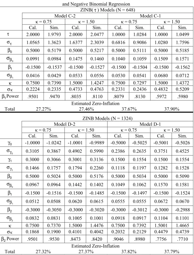
The ZINB(_τ) and ZINB models consisted of the same parameter estimates as the ZIP(_τ) and ZIP models (Model C-τ and Model D-τ), but included an extra scale parameter,

0.75

κ = and _{κ =}1.50. SAS programming code to evaluate a large sample simulation for distributional characteristics, to construct an expanded data set, and to calculate power, for models with a continuous covariate related to the zero-inflation are presented in Appendices C and D, for the Poisson and negative binomial regression models, respectively.

The results of the ZIP(_τ) and ZIP models with a continuous covariate for zero- inflation are presented in Table 3. As before, when _τ decreases, based on the same sample size and value of the regression coefficient tested, the calculated power is reduced, and there is also a slight tendency for the simulated data to result in inflated average parameter estimates for the standard error (_σ_τ) with the ZIP(_τ) models, and with inflated average parameter estimates of the standard errors for the logistic portion involving zero-inflation ( 0 γ σ and 1 γ σ ) with the ZIP models.

The results of the ZINB(_τ) and ZINB models with a continuous covariate for zero-inflation are presented in Table 4. Similar to the results previously presented, based on the same sample size and value of the regression coefficient tested, whenτdecreases and/or when overdispersion of the non-zero counts increases, the calculated power is reduced There is a slight tendency for simulated data to result in inflated average standard errors (_σ_τ) for the parameter estimates of _τwith the ZINB(_τ) models, and with inflated average standard errors (

0

γ σ and

1

γ

σ ) for the logistic portion involving zero-inflation (_γ₀ and _γ₁) with the ZINB models.

Conclusion

Examples of ZIP, ZIP(τ), ZINB and ZINB(τ) models were used to extend the method of estimating conditional power presented by Lyles, et al. (2007) to zero-inflated count data. Utilizing the variance-covariance matrix of the

model fitted to an expanded data set, power was estimated for the Wald statistic. Although not presented here, this method can also be used to approximate power based on the likelihood ratio test. Overall, with the same sample size and parameter value of the estimate of interest to be tested with the Wald test statistic, results indicated a decrease in power as the percent of zero-inflation and/or over-dispersion increased. This trend was particularly more noticeable for the ZIP(τ) and ZINB(τ) models. Calculated power estimates indicate if the percent of zero-inflation or over-dispersion is underestimated, a loss of assumed power in the statistical test will result.

To estimate power for zero-inflated count data it is necessary to select a value of τ

for the ZIP(τ) and ZINB(τ) models or values of the regression coefficients associated with the logistic portion in the ZIP and ZINB models (i.e.,_γ₀and_γ₁) to produce the correct assumed proportion of zero-inflation. But in practice, these parameter values may be unknown or difficult to estimate. Generating a large simulated data set iteratively until the expected percent of zero-inflation occurs can aid the researcher in obtaining approximations to the population distributional characteristics of model and estimation of the parameter values associated with zero-inflation can be improved.

References

Cameron, A. C., & Trivedi, P. K. (2006).

Regression analysis of count data. New York: Cambridge University Press.

Greene, W. H. (1994). Accounting for excess zeros and sample selection in Poisson and negative binomial regression models. Stern School of Business, New York University, Dept. of Economics Working Paper, No. EC-94-10.

Lambert, D. (1992). Zero-inflated Poisson regression, with an application to defects in manufacturing. Technometrics, 34, 1-14.

Lord, D. (2006). Modeling motor vehicle crashes using Poisson-gamma models: Examining the effects of low sample mean values and small sample size on the estimation of the fixed dispersion parameter. Accident Analysis and Prevention, 38, 751-766.

(13)

371

Lyles, R. H., Lin, H-M., & Williamson J. M. (2007). A practical approach to computing power for generalized linear models with nominal, count, or ordinal responses. Statistics in Medicine, 26, 1632-1648.

SAS Institute, Inc. (2004). SAS/STAT 9.1 User’s Guide. SAS Institute Inc: Cary, NC.

Appendix A:

SAS Code with a Binary Covariate for Zero-Inflation and Poisson Regression

Step 1: Evaluate a large sample simulation for distributional characteristics.

ZIP(_τ)

data ziptau1; seed = 12345;

lambda1 = 2; lambda2 = 1.4; tau = 2; n = 100000;

beta0 = log(lambda1);

beta1 = log(lambda2) - log(lambda1); do x = 0 to 1; do i = 1 to n;

lambda = exp(beta0 + beta1*x);

prob_0 = exp(-tau*beta0 - tau*beta1*x)/ (1 + exp(-tau*beta0 - tau*beta1*x)); zero_inflate = ranbin(seed,1,prob_0); if zero_inflate = 1 then y = 0;

else y = ranpoi(seed,lambda);

if zero_inflate = 0 then yPoisson = y; else yPoisson = .;

output; end; end; proc sort; by x;

proc freq; tables y zero_inflate; by x; run; proc freq; tables zero_inflate; run; proc means mean var n; var y yPoisson; by x; run;

ZIP

data zip1; seed = 12345;

beta1 = log(lambda2) - log(lambda1); beta2 = beta1;

gamma0 = -tau*beta0; gamma1 = -tau*beta1;

do x = 0 to 1; do z = 0 to 1; do i = 1 to n; lambda = exp(beta0 + beta1*z + beta2*x); prob_0 = exp(gamma0 + gamma1*z)/ (1 + exp(gamma0 + gamma1*z)); zero_inflate = ranbin(seed,1,prob_0);

if zero_inflate = 1 then y=0; else y = ranpoi(seed,lambda); if zero_inflate = 0 then yPoisson = y; else yPoisson=.;

output; end; end; end; proc sort; by x z;

proc freq; tables y zero_inflate; by x z; run; proc means mean var n; var y yPoisson; by x z; run;

proc sort; by z;

proc freq; tables zero_inflate; by z; run; proc freq; tables zero_inflate; run;

Step 2: Construct an expanded data set to approximate conditional power.

ZIP(_τ) data ziptau2;

lambda1 = 2; lambda2 = 1.4; tau = 2; totaln = 212; numgroups = 2;

n = totaln/numgroups; increment = 10; beta0 = log(lambda1);

beta1 = log(lambda2) - log(lambda1); do x = 0 to 1;

if x = 0 then j = 13; if x = 1 then j = 9; do i = 1 to n;

prob_0 = exp(-tau*beta0 - tau*beta1*x)/ (1 + exp(-tau*beta0 - tau*beta1*x)); do y = 0 to j + increment;

if y = 0 then w = prob_0 + (1-prob_0) *(exp(-lambda)*lambda**y)/gamma(y + 1);

if y > 0 then w = (1-prob_0)*(exp (-lambda)*lambda**y)/gamma(y + 1); output; end; end; end;

proc nlmixed tech=dbldog cov; parameters t=3 b0=0 b1=0;

p0 = exp(t*b0 t*b1*x)/(1 + exp(t*b0 -t*b1*x)); mu = exp(b0 + b1*x);

if y = 0 then do;

ll = (log(p0 + (1 - p0)*exp(-mu))); end; if y > 0 then do;

ll = (log(1 p0) + y*log(mu) lgamma(y + 1) -mu); end; loglike = w*ll;

model y ~ general(loglike); run; ZIP

data zip2;

lambda1 = 2; lambda2 = 1.4; tau = 2; totaln = 488; numgroups = 4;

(14)

372

n = totaln/numgroups; increment = 10; beta0 = log(lambda1);

beta1 = log(lambda2) - log(lambda1); beta2 = beta1; gamma0 = -tau*beta0; gamma1 = -tau*beta1; do x = 0 to 1; do z =0 to 1; if x = 0 and z = 0 then j = 13; if x = 0 and z = 1 then j = 9; if x = 1 and z = 0 then j = 8; if x = 1 and z = 1 then j = 7; do I = 1 to n;

lambda = exp(beta0 + beta1*z + beta2*x); prob_0 = exp(gamma0 + gamma1*z)/ (1 + exp(gamma0 + gamma1*z)); do y = 0 to j + increment ;

if y = 0 then w = prob_0 + (1-prob_0)* (exp(-lambda)*lambda**y)/gamma(y + 1); if y > 0 then w = (1-prob_0)*(exp(-lambda) *lambda**y)/gamma(y + 1);

output; end; end; end; end; proc nlmixed tech=dbldog cov;

parameters g0=0 g1=0 b0=0 b1=0 b2=0; p0 = exp(g0 + g1*z)/(1 + exp(g0 + g1*z)); mu = exp(b0 + b1*z + b2*x);

if y = 0 then do;

ll = (log(p0 + (1 - p0)*exp(-mu))); end; if y > 0 then do;

ll = (log(1 - p0) + y*log(mu) - lgamma(y + 1) - mu); end; loglike = w*ll;

model y ~ general(loglike); run; Step 3: Calculate power.

data power; estimate = -0.3567; standerr = 0.0989;

eta = (estimate**2)/(standerr**2); critvalue = cinv(.95,1);

power = 1-probchi(critvalue,1,eta); proc print; var eta power; run;

Appendix B:

SAS Programming Code with a Binary Covariate for Zero-Inflation and Negative

Binomial Regression

ZINB(_τ)

data zinbtau1; seed = 12345;

beta1 = log(lambda2) - log(lambda1); kappa = .75; delta = 1/kappa;

do x = 0 to 1; do i = 1 to n; lambda = exp(beta0 + beta1*x); phi = 1/delta*rangam(seed,delta); theta = lambda*phi;

prob_0 = exp(-tau*beta0 - tau*beta1*x)/ (1 + exp(-tau*beta0 - tau*beta1*x)); zero_inflate = ranbin(seed,1,prob_0); if zero_inflate = 1 then y = 0;

else y = ranpoi(seed,theta);

if zero_inflate = 0 then yPoisson = y; else yPoisson = .; output; end; end; proc sort; by x;

proc freq; tables y zero_inflate; by x; run; proc freq; tables zero_inflate; run; proc means mean var max; var y yPoisson; by x; run;

proc means mean var n; var y yPoisson; run; ZINB

data zinb1; seed = 12345;

lambda1 = 2; lambda2 = 1.4; tau = 2; n = 100000; kappa = .75; delta = 1/kappa; beta0 = log(lambda1);

beta1 = log(lambda2) - log(lambda1); beta2 = beta1;

gamma0 = -tau*beta0; gamma1 = -tau*beta1;

do x = 0 to 1; do z = 0 to 1; do i = 1 to n; lambda = exp(beta0 + beta1*z + beta2*x); phi = 1/delta*rangam(seed,delta);

theta = lambda*phi;

prob_0 =exp(gamma0 + gamma1*z)/ (1 + exp(gamma0 + gamma1*z)); zero_inflate = ranbin(seed,1,prob_0); if zero_inflate = 1 then y = 0;

else y = ranpoi(seed, theta);

if zero_inflate = 0 then yPoisson = y; else yPoisson = .; output; end; end; end; proc sort; by x z;

proc freq; tables y zero_inflate; by x z; run; proc means mean var max n;

var y yPoisson; by x z; run; proc sort; by z;

proc freq; tables y zero_inflate; by z; run; proc freq; tables y zero_inflate; run;

(15)

373

ZINB(_τ) data zinbtau2;

lambda1 = 2; lambda2 = 1.4; tau = 2; totaln = 464; numgroups = 2; kappa = .75; n = totaln/numgroups; increment = 8; beta0 = log(lambda1);

beta1 = log(lambda2) - log(lambda1); do x = 0 to 1;

prob_0 = exp(-tau*beta0 - tau*beta1*x)/ (1 + exp(-tau*beta0 - tau*beta1*x)); do y = 0 to j + increment;

if y = 0 then w = prob_0 + (1-prob_0) * gamma(kappa**-1 + y)/

(gamma(kappa**-1)*gamma(y+1))* ((kappa*lambda/(1 + kappa*lambda))**y) *((1/(1 + kappa*lambda))**(1/kappa));

if y > 0 then w = (1-prob_0)* gamma(kappa**-1 + y)/(gamma(kappa**-1)*gamma(y+1))* ((kappa*lambda/(1 + kappa*lambda))**y) *((1/(1 + kappa*lambda))**(1/kappa)); output; end; end; end;

proc nlmixed tech=dbldog cov; parameters t=3 b0=0 b1=0 k=1; p0 = exp(-t*b0 - t*b1*x)/(1 + exp(-t*b0 - t*b1*x)); mu = exp(b0 + b1*x); if y = 0 then do; ll = p0 + (1-p0)*exp(-(y+(1/k))* log(1+k*mu)); end; if y > 0 then do; ll = (1-p0)*exp(lgamma(y+(1/k)) - lgamma(y+1) - lgamma(1/k) + y*log(k*mu) - (y + (1/k)) * log(1 + k*mu)); end;

loglike = w * log(ll);

model y ~ general(loglike); run; ZINB

data zinb2;

lambda1 = 2; lambda2 = 1.4; tau = 2; totaln = 928; numgroups=4; kappa = .75; n = totaln/numgroups; increment = 5; beta0 = log(lambda1);

beta1 = log(lambda2) - log(lambda1); beta2 = beta1; gamma0 = -tau*beta0; gamma1 = -tau*beta1; do x = 0 to 1; do z = 0 to 1; if x = 0 and z = 0 then j = 29; if x = 0 and z = 1 then j = 20; if x = 1 and z = 0 then j = 21; if x = 1 and z = 1 then j = 14; do i = 1 to n;

lambda = exp(beta0 + beta1*z + beta2*x); prob_0 = exp(gamma0 + gamma1*z)/ (1 + exp(gamma0 + gamma1*z)); do y = 0 to j + increment;

if y = 0 then w = prob_0 + (1-prob_0) * gamma(kappa**-1 + y)/(gamma(kappa**-1)*gamma(y+1))*

((kappa*lambda/(1 + kappa*lambda))**y) *((1/(1 + kappa*lambda))**(1/kappa));

if y > 0 then w = (1-prob_0)* gamma(kappa**-1 + y)/(gamma(kappa**-1)*gamma(y+1))* ((kappa*lambda/(1 + kappa*lambda))**y) *((1/(1 + kappa*lambda))**(1/kappa)); output; end; end; end; end;

proc nlmixed tech=dbldog cov;

parameters g0=0 g1=0 b0=0 b1=0 b2=0 k=1; p0 = exp(g0 + g1*z) / (1 + exp(g0 + g1*z)); mu = exp(b0 + b1*z + b2*x); if y = 0 then do; ll = p0 + (1-p0)*exp(-(y+(1/k))* log(1+k*mu)); end; if y > 0 then do; ll = (1-p0)*exp(lgamma(y+(1/k)) - lgamma(y+1) - lgamma(1/k) + y*log(k*mu) - (y + (1/k)) * log(1 + k*mu)); end;

eta = (estimate**2)/(standerr**2); critvalue = cinv(.95,1);

power = 1 - probchi(critvalue,1,eta); proc print; var eta power; run;

Appendix C:

SAS Code with a Continuous Covariate for Zero-Inflation and Poisson Regression Step 1: Evaluate a large sample simulation for distributional characteristics.

(16)

374

ZIP(_τ)

data ziptau3; seed = 12345; tau = 2; n = 100000;

beta0 = .50; beta1 = -.15; do i = 1 to n;

z = rannor(seed);

lambda = exp(beta0 + beta1*z);

prob_0 = exp(-tau*beta0 - tau*beta1*z)/ (1 + exp(-tau*beta0 - tau*beta1*z)); zero_inflate = ranbin(seed,1,prob_0); if zero_inflate = 1 then y = 0; else y = ranpoi(seed, lambda); if zero_inflate = 0 then yPoisson=y; else yPoisson = .;

output; end;

proc freq; tables y zero_inflate; run;

proc means mean var n; var y yPoisson; run; ZIP

data zip3; seed = 12345; tau = 2; n = 100000; beta0 = .50; beta1 = -.15; beta2 = 2 * beta1; gamma0 = -tau*beta0; gamma1 = -tau*beta1; do x = 0 to 1; do i = 1 to n; z = rannor(seed);

lambda = exp(beta0 + beta1*z + beta2*x); prob_0 = exp(gamma0 + gamma1*z)/ (1 + exp(gamma0 + gamma1*z)); zero_inflate = ranbin(seed,1,prob_0); if zero_inflate = 1 then y = 0; else y = ranpoi(seed, lambda); if zero_inflate = 0 then yPoisson=y; else yPoisson = .;

output; end; end;

proc freq; tables y zero_inflate; run; proc sort; by x;

proc freq; tables y; by x; run;

proc means mean var n; var y yPoisson; by x; run;

ZIP(_τ) data ziptau4; tau = 2; n = 302; j = 11; beta0 = .50; beta1 = -.15; increment = 10; do i = 1 to n; z = probit((i - 0.375)/( n + 0.25)); lambda = exp(beta0 + beta1*z);

prob_0 = exp(-tau*beta0 - tau*beta1*z)/ (1 + exp(-tau*beta0 - tau*beta1*z)); do y = 0 to j + increment;

if y = 0 then w = prob_0 + (1-prob_0) *(exp(-lambda)*lambda**y)/gamma(y+1);

if y > 0 then w = (1-prob_0)*(exp (-lambda)*lambda**y)/gamma(y+1); output; end; end;

proc nlmixed tech=dbldog cov; parameters t=3 b0=0 b1=0;

p0 = exp(-t*b0 - t*b1*z)/(1 + exp(-t*b0 - t*b1*z)); mu = exp(b0 + b1*z); if y = 0 then do;

ll = (log(p0 + (1-p0)*exp(-mu))); end; if y > 0 then do;

ll = (log(1-p0) + y*log(mu) - lgamma(y+1) - mu); end; loglike = w * ll;

model y ~ general(loglike); run; ZIP

data zip4;

tau = 2; totaln = 694; numgroups=2; n = totaln/numgroups; increment = 10; beta0 = .50; beta1 = -.15; beta2 = 2* beta1; gamma0 = -tau*beta0; gamma1 = -tau*beta1; do x = 0 to 1; if x = 0 then j = 11; if x = 1 then j = 9; do i = 1 to n; z = probit((i -0.375)/(n + 0.25));

lambda = exp(beta0 + beta1*z + beta2*x); prob_0 = exp(gamma0 + gamma1*z)/ (1 + exp(gamma0 + gamma1*z)); do y = 0 to j + increment ;

if y = 0 then w = prob_0 + (1-prob_0) *(exp(-lambda)*lambda**y)/gamma(y+1);

if y > 0 then w = (1-prob_0)*(exp (-lambda)*lambda**y)/gamma(y+1); output; end; end; end;

parameters g0=0 g1=0 b0=0 b1=0 b2=0; p0 = exp(g0 + g1*z)/(1 + exp(g0 + g1*z)); mu = exp(b0 + b1*z + b2*x);

if y = 0 then do;

ll = (log(p0 + (1-p0)*exp(-mu))); end; if y > 0 then do;

ll = (log(1-p0) + y*log(mu) - lgamma(y+1)- mu); end; loglike = w * ll;

(17)

375

eta = (estimate**2)/(standerr**2); critvalue=cinv(.95,1);

power=1-probchi(critvalue,1,eta); proc print; var eta power; run;

Appendix D:

SAS Programming Code with a Continuous Covariate for Zero-Inflation and Negative

Binomial Regression

ZINB(_τ)

data zinbtau3; seed = 12345; tau = 2; n = 100000;

beta0 = .50; beta1 = -.15; kappa = .75; delta = 1/kappa; do i = 1 to n;

z = rannor(seed);

lambda = exp(beta0 + beta1*z); phi = 1/delta*rangam(seed,delta); theta = lambda*phi;

prob_0 = exp(-tau*beta0 - tau*beta1*z)/ (1 + exp(-tau*beta0 - tau*beta1*z)); zero_inflate = ranbin(seed,1,prob_0); if zero_inflate = 1 then y = 0;

if zero_inflate=0 then yPoisson=y; else yPoisson=.; output; end;

proc freq; tables y zero_inflate; run;

proc means mean var max n; var y yPoisson; run;

ZINB

data zinb3; seed = 12345; tau = 2; n = 100000; beta0 = .50; beta1 = -.15; beta2 = 2 * beta1; gamma0 = -tau*beta0; gamma1 = -tau*beta1; kappa = .75; delta = 1/kappa; do x = 0 to 1;

do i = 1 to n; z = rannor(seed);

lambda = exp(beta0 + beta1*z + beta2*x); phi = 1/delta*rangam(seed,delta);

theta = lambda*phi;

prob_0 = exp(gamma0 + gamma1*z)/ (1 + exp(gamma0 + gamma1*z)); zero_inflate = ranbin(seed,1,prob_0); if zero_inflate = 1 then y = 0;

if zero_inflate=0 then yPoisson=y; else yPoisson=.; output; end; end; proc sort; by x;

proc freq; tables y zero_inflate; by x; run; proc freq; tables y zero_inflate; run;

proc means mean var max n; var y yPoisson; by x; run;

proc means mean var n; var y yPoisson; run; Step 2: Construct an expanded data set to approximate conditional power.

ZINB(_τ) data zinbtau4; tau = 2; n = 648; beta0 = .5; beta1 = -.15; kappa = .75; j = 23; increment = 7; do i = 1 to n; z = probit((i - 0.375)/( n + 0.25)); lambda = exp(beta0 + beta1*z);

prob_0 = exp(-tau*beta0 - tau*beta1*z)/ (1 + exp(-tau*beta0 - tau*beta1*z)); do y = 0 to j + increment;

if y = 0 then w = prob_0 + (1-prob_0) * gamma(kappa**-1 + y)/(gamma(kappa**-1)*gamma(y+1))* ((kappa*lambda/(1 + kappa*lambda))**y) *((1/(1 + kappa*lambda))**(1/kappa)); if y > 0 then w = (1-prob_0)* gamma(kappa**-1 + y)/(gamma(kappa**-1) *gamma(y+1))* ((kappa*lambda/(1 + kappa*lambda))**y) *((1/(1 + kappa*lambda))**(1/kappa)); output; end; end;

proc nlmixed tech=dbldog cov; parameters t=3 b0=0 b1=0 k=1; p0 = exp(-t*b0 - t*b1*z)/(1 + exp(-t*b0 - t*b1*z)); mu = exp(b0 + b1*z); if y = 0 then do; ll = p0 + (1-p0)*exp(-(y+(1/k))* log(1+k*mu)); end; if y > 0 then do; ll = (1-p0)*exp(lgamma(y+(1/k)) - lgamma(y+1) - lgamma(1/k) + y*log(k*mu)- (y + (1/k)) * log(1 + k*mu)); end;

(18)

376

model y ~ general(loglike); run; ZINB

data zinb4;

totaln = 1324; numgroups = 2; n = totaln/numgroups; tau = 2;

beta0 = .5; beta1 = -.15; beta2 = 2*beta1; gamma0 = -tau*beta0; gamma1 = -tau*beta1; kappa = .75; increment = 5;

do x = 0 to 1;

z = probit((i - 0.375)/( n + 0.25));

lambda = exp(beta0 + beta1*z + beta2*x); prob_0 = exp(gamma0 + gamma1*z)/ (1 + exp(gamma0 + gamma1*z)); do y = 0 to j + increment;

if y = 0 then w = prob_0 + (1-prob_0) * gamma(kappa**-1 + y)/

(gamma(kappa**-1) *gamma(y+1))* ((kappa*lambda/(1 + kappa*lambda))**y) *((1/(1 + kappa*lambda))**(1/kappa));

if y > 0 then w = (1-prob_0)* gamma(kappa**-1 + y)/(gamma(kappa**-1)*gamma(y+1))* ((kappa*lambda/(1 + kappa*lambda))**y) *((1/(1 + kappa*lambda))**(1/kappa)); output; end; end; end;

parameters g0=0 g1=0 b0=0 b1=0 b2=0; p0 = exp(g0 + g1*z)/(1 + exp(g0 + g1*z)); mu = exp(b0 + b1*z + b2*x); if y = 0 then do; ll = p0 + (1-p0)*exp(-(y+(1/k))* log(1+k*mu)); end; if y > 0 then do; ll = (1-p0)*exp(lgamma(y+(1/k)) - lgamma(y+1) - lgamma(1/k) + y*log(k*mu)- (y + (1/k)) * log(1 + k*mu)); end;

eta = (estimate**2)/(standerr**2); critvalue=cinv(.95,1);

power=1-probchi(critvalue,1,eta); proc print; var eta power; run;