Robust Support Vector Machines For Implicit Outlier Removal

(1)

Master of Science Thesis

Examiners: Dr. Tech. Ari Visa

M.Sc. Mikko Parviainen Examiners and topic approved in the Department of Signal Processing meeting on 7th November 2012

(2)

ABSTRACT

TAMPERE UNIVERSITY OF TECHNOLOGY

Master's Degree Programme in Information Technology

FERDINAND KAISER: Robust Support Vector Machines For Implicit Outlier Removal

Master of Science Thesis, 42 pages, 8 Appendix pages November 2012

Major: Signal processing

Examiner: Dr. Tech. Ari Visa, M.Sc. Mikko Parviainen

Keywords: Support Vector Machine, Robustness, Truncated Hinge Loss Function The support vector machine is a machine learning algorithm which has been suc-cessfully applied to solve classication problems since its introduction in the early 1990s. It is based on the work of Vladimir Vapnik on Statistical Learning Theory and is theoretically well founded. Following the discriminative approach, the SVM yields a classier which separates two classes by a hyperplane. The training in-stances are classied according to the sign of their distance to the hyperplane. This hyperplane is dened by a small number of training instances such that the distance of the training instances of both classes to the hyperplane is maximized and the misclassication error is minimized. Hence the support vector machine belongs to the family of maximum margin classiers. Since the support vector machine does not estimate the underlying class conditional distribution of the training instances, but instead uses them directly to construct the classier, it is important that the training instances are sampled from the underlying class conditional distribution. If this is not the case because the training set is contaminated with outliers, the accu-racy of the classier dened by the support vector machine decreases. Based on this observation several approaches have been proposed to improve the robustness of the support vector machine against outliers in the training data. In this thesis we will discuss the class robust support vector machines which aim to make the standard support vector machine robust against noise by implicit outlier ltering. Those ap-proaches are using the support vector machine to detect and remove outliers based on their position relative to the separating hyperplane. Since the success of those methods is only empirically proven, we conduct a thoroughly experimental study in order to determine under which conditions those robust methods can be applied in practice. We are especially interested if the additional parameter which controls the removal of outliers can be estimated from a training set which is contamined by outliers.

(3)

I would like to thank my thesis supervisor Dr. Tech. Ari Visa for all the good advices and insights during the thesis process. And of course I also want to thank my family and my girlfriend for their love and constant support.

Ferdinand Kaiser

(4)

LIST OF TABLES

4.1 Dimensionality and size of the training and test sets used for evaluation 33 A.1 Classication accuracies using the linear kernel on datasets contamined

by class noise . . . 47 A.2 Classication accuracies using the RBF kernel on datasets contamined

by class noise . . . 48 A.3 Classication accuracies using the linear kernel on datasets contamined

by adversarial noise . . . 49 A.4 Classication accuracies using the RBF kernel on datasets contamined

by adversarial noise . . . 50 A.5 Number of support vectors and F1-scores using the linear kernel on

datasets contamined by class noise . . . 51 A.6 Number of support vectors and F1-scores using the RBF kernel on

datasets contamined by class noise. . . 52 A.7 Number of support vectors and F1-scores using the linear kernel on

datasets contamined by adversarial noise. . . 53 A.8 Number of support vectors and F1-scores using the RBF kernel on

(7)

CCCP Constrained Concave-Convex Procedure CV Cross-Validation

ERM Empirical Risk Minimization KKT conditions Karush-Kuhn-Tucker conditions

RBF Radial Basis Function SLT Statistical Learning Theory SRM Structural Risk Minimization VC-dimension Vapnik-Chervonenkis dimension

(8)

1. INTRODUCTION

Learning from examples, also known as supervised learning, requires to infer a deci-sion rule from examples. If we assume that some examples presented to the learner are erroneous or in other words outliers with respect to the other examples, the learner needs to be able to detect them. Suppose a human wants to learn how to discriminate between two dierent classes of owers given a set of labeled exam-ples. Based on some features of the owers such as color or smell and the label provided by the teacher, a human nds a way how to distinguish between those two species eectively. If some of the examples are incorrectly labeled, a human would notice that those mislabeled examples are more similar to the other class than to the actual class label. Consequently those examples would be excluded from the learning process. This ability to detect training examples which are highly unlikely to occur and which contradict the general distribution of the data is essential in supervised learning, since real world data is often polluted by a certain amount of errors. Those errors are either introduced by mislabeling through the teacher as mentioned above, or by measurement errors during the acquisition of the features. The way a human would recognize outliers is based on certain assumptions. One assumption could be that the examples belonging to one class should not dier too much in their features. Consequently learning algorithms designed to be executed by computers need to include methods in order to identify erroneous training examples. In this thesis we show how supervised learning is implemented by a specic learn-ing algorithm, the support vector machine. Furthermore we present a specic class of approaches which have been proposed in order to make this learning algorithm robust against outliers in the training data. Dierent from the example above the robust methods we are focusing on do not rely on a specic assumption about the distribution of the data, but implicitly remove outliers during the training process of the classier. In the experimental part of this thesis we evaluate how accurately the outliers are detected and under which conditions the robust methods improve the performance of the support vector machine. This evaluation is based on real-world datasets which are contamined with outliers. We measure the classication accuracy of the support vector machine and the robust approaches as well as the accuracy of outlier removal in order to compare the dierent classiers.

(9)

1.0.1 Thesis Outline

This thesis is divided into six chapters. In chapter two we discuss the theoretical background of support vector machines, the dierent types of support vector ma-chines as well as the robustness property of the standard support vector machine. Chapter three introduces the dierent approaches to integrate outlier removal into the training of the standard support vector machine by using alternative loss func-tions. In the fourth chapter the experimental setup is described, followed by the fth chapter were the experimental results are discussed. The last chapter summarizes our ndings.

(10)

2. THEORETICAL BACKGROUND

2.1 Supervised Learning

Learning machines which are trained based on a set of instances x and labels y belong to the family of supervised learning algorithms. Figure 2.1 explains the model of the supervised learning setting. The model consists of a generator G which samples instancesx independently from a unknown xed distribution P (X)

and a supervisor T which assigns an output value y to x according to a xed un-known distributionP (Y|X). The learning machine observes a set of training pairs

S = {(x1, y1),(x2, y2). . .(xl, yl)}. Based on the presented examples the learning

machine selects a functionh:X → Y from a class of functionsHsuch as to

approx-imate the output of T as good as possible for any given x. The functionh is called the hypothesis. The process of choosing an appropriate hypothesis from a class of Hypothesis H is where the machine is learning [22] and is denoted as the training of the classier.

Supervised learning algorithms dier in how learning is performed and how the training pairs are presented to the learner. It is distinguished between batch learn-ing, online learning and active learning. In this thesis we will focus on batch learning which assumes the training set is xed and all training samples are independently and identically distributed, that is the learning process has no inuence on the com-position of the training set.

Depending on the type of output valuesythe class of supervised learning problems is distinguished classication and regression problems. In classication problems the output spaceY is a set of discrete values whereas regression problems deal with

continuous outputs

h:X → {−1,1} , X =_Rn. (2.1)

In classication problems the hypothesis is also denoted as decision function or just the classier. The aim is to nd a hypothesis which performs good not only on the training data but on all the data, that is the hypothesis should make as little

(11)

Generator

Teacher

Learning

Machine

y

Figure 2.1: Flowchart of supervised learning taken from [22]. The learning machine is trained with pairs (x,y). The input variable x is sampled by a generator process G and labeled by a supervisor T. The aim is to mimic the behaviour of the supervisor as good as possible.

misclassication errors as possible on unseen data. In order to quantify how good a hypothesis performs we measure the expected error further on called the expected risk. For binary classication we can simply use the 0-1 loss-function or Boolean error dened as L0−1(h(xi), yi) =    0 h(xi) = yi 1 h(xi)6=yi (2.2) As we see later the type of loss-function used during the training aects several aspects e.g. the robustness of the learning machine to noise and the uniqueness of the found solution. Using the 0-1 loss function we dene the expected risk which is equal to the probability of misclassication for binary problems

R(h) = E(L0−1(h(x), y)) = Z L0−1(h(x), y)dP (x, y) = Z Z L0−1(h(x), y)dP (y|x)dP (x) (2.3) The expected risk is a measure of how likely the misclassication of an input sam-ple is over all possible inputs. Intuitively the expected risk of the classier should be as low as possible. From this point of view learning in general is a risk minimiza-tion problem, the best classier is selected based on the training data in order to minimize the risk.

There are two dierent methods to nd the appropriate hypothesish which min-imizes the estimated risk. The rst one is to imitate the supervisors behavior by

(12)

Figure 2.2: A classication problem in two dimensional space which is dicult to solve using generative approaches (UCI Fourclass dataset)

directly nding a mapping from X → Y. Learning machines which nd this direct

mapping are called discriminative methods such as the support vector machine or the perceptron algorithm. The second one is to identify the behavior of the su-pervisor by modeling the distributions of the input and output variables in order to minimize the expected risk. Those methods are referred to as generative or paramet-ric approaches such as the Naive Bayes classier. The generative and discriminative approaches dier in complexity and in the kind of prior knowledge which can be incorporated in the classier design.

Generative Learning algorithms consist of two stages. In the inference stage the class-conditional probabilities p(x|y) as well as p(y) and p(x) are estimated from

the training examples. The problem is to nd the parameters of a given family of distributions that explain the given observations in the best possible way, one solution is to nd the parameters such that the observations becomes most likely. Based on those distributions the posterior class probabilities p(y|x) are determined

for each class using the Bayes law. In a second stage decision theory is used in combination with p(y|x) to nd the class-membership of the unknown instance x [4]. Vapnik describes the rst step as from particular to general (inductive) and the second step as from general to particular (deductive step) [22]. The disadvantage of the generative algorithms is that modeling p(x|y) can be dicult, especially given

(13)

problem where it is dicult to model p(x|y). The advantages of generative

ap-proaches is that abnormal points in the training set can be identied by evaluating p(x).

The discriminative methods nd the discriminative function mapping from X → Y

directly based on the training set S, they do not try to model the distributions of the input and output variables. The complexity of the stated problem is lower since only the one direct step must be solved. The advantage is that we do not face the curse of dimensionality by trying to parameterize a distribution in a high-dimensional input space. On the other hand we can not utilize the posterior probabilities p(y|x) in

order to determine how condent the classier is, given a specic value ofx.

As mentioned earlier the overall goal is to minimize the expected risk, the prob-lem is that the joint probability distribution is unknown p(x, y). Discriminative

approaches solving a classication problem therefore minimize the empirical risk insteadRemp of the expected risk dened as

Remp(h) = ˆE(L0−1(f(X), Y)) = 1 l l X i=1 L0−1(h(xi), yi) ,(xi, yi)∈S (2.4)

However if the selection of the best hfrom the class of all possible hypothesis H is solely based on the empirical error, it is not guaranteed that the expected risk is minimized [20]. To see this imagine a hypothesis which yields a zero training error by remembering all training examples, nothing is learned about the underlying con-cept of the problem and we risk to fail in classifying unseen examples correctly. This problem is typical for supervised learning and referred to as overtting. In order to avoid overtting and enforce a small number expected errors on unseen data, the learning machine must be able to generalize well or in other words to have a small generalization error |R(h)−Remp(h)| [24], again this requirement can not be used

directly to select the best hypothesis since the expected risk R is unknown.

To summarize this section, the goal of machine learning is to learn the underlying dependencies between input and output variables as good as possible by generalizing from the training data. In order to learn this dependence empirical risk minimization is applied. The open questions is what are conditions for good generalization. This question was answered by Vapnik within his work on Statistical Learning Theory which led to the development of support vector machines, in the following the main ndings of the statistical learning theory are described.

(14)

2.2 Statistical Learning Theory

Learning theory is a eld of theoretical computer science and analyzes machine learning algorithms. A learning theory is used as a framework to determine which kind of problems are learnable by a given algorithm and how good (convergence rates, bounds on the error) this learning is. Some examples of learning theories are Bayesian leaning, probably approximately correct learning and the statistical learn-ing theory (SLT). The SLT rst introduced by Vladimir Vapnik in the late 1960s [22], is a general learning theory which considers classication, regression and den-sity estimation problems as special cases. Vapnik analyzed the principle of inductive inference on a mathematical basis in order to nd conditions under which the law of large numbers holds for a hypothesis class. Namely among what conditions the empirical risk of a hypothesis chosen from a hypothesis class converges to the true risk. Based on the empirical risk minimization, that is used by all inductive learning algorithms, he determined conditions under which the learning process is consistent, bounds on generalization and how the generalization rate of a learning machine can be controlled. In his analysis he focused especially on how learning should be per-formed in the case of small training sample sizes, and models the problem of learning as a direct learning approach. His intention is to solve the learning problem directly, if the amount of information is restricted and to never solve a more general problem as an intermediate step [22].

2.2.1 Empirical Risk Minimization

The problem of empirical risk minimization (ERM) is to nd the hypothesis hl

from a class of functionsH which minimizes the empirical risk. Statistical learning theory was developed by applying the direct method, therefore the empirical risk minimization is done based on problem formulation in 2.5. Given a collection of training samples S of size l, we determine the best hypothesis hl by minimizing

hl = arg minRemp(h) = 1 l l X i=1 L(h(xi), yi) ,(xi, yi) (2.5)

Dierent from equation 2.4 the above equation uses a general loss function since the SLT is a general learning theory independent of the specic learning problem solved, it can be applied to classication as well as regression or density estimation.

(15)

R

R_emp

inf R

number of training samples

Risk

Figure 2.3: Empirical process is consistent if the expected and empirical risk converge to the minimal possible value of the Risk, after [22]

2.2.2 Consistency

Consistency is a general property of a learning process, in order to dene it we introduce two classiers.

Leth_H be the best classier inH the one which minimizes the expected risk and lethl be the classier selected fromH based on a set of training examples

h_H = arg minR(h)

hl = arg minRemp(h)

A learning method is consistent if the following two conditions are fullled R(hl)→Pl→inf R(hH)Remp(hl)→Pl→inf R(hH) (2.6) This means that if the number of training samples is increased to innity, the expected risk of the classier produced by the learning machine must converge to the best achievable solution given the function class H. Furthermore the empirical risk of the classier must converge to this expected risk as shown in gure 2.3. As pointed out by Luxburg et al.[24] consistency is therefore a property of H and not of a single function h. Vapnik showed that if hl is determined based on empirical

risk minimization the necessary and sucient condition for consistency is uniform convergence of Remp(f) to R(f) for all possible hypothesis h∈ H as shown in the

next equation lim l→∞P sup f∈_F |R(f)−Remp(f)| ≥ →0, ∀ (2.7)

(16)

0 5 10 0 2 4 6 8 10 0 5 10 0 2 4 6 8 10 0 5 10 0 2 4 6 8 10

Figure 2.4: An overtting example

.

This means that for all hypotheses h in hypothesis class of H it holds that by increasing the amount of training data the empirical risk of the hypothesis approxi-mates the true risk. In that sense the requirement for consistency of ERM is that the law of large numbers takes place in the hypothesis class H for all h simultaneously since the hypothesishl is not xed due to its dependence on the training set. Thus

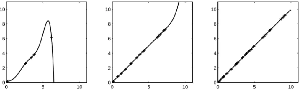
the consistency, that is success of the empirical risk minimization depends, on the generalization ability of the specic hypothesis classHused in the learning process. In order to illustrate a case which violates this condition, let us have a look at the overtting example of gure 2.4. All three hypotheses yield zero training error Remp(h) = 0, but only one of them also minimizes the expected error. In this

specic example training sets of sizes of 5, 10 and 15 were used. The hypothesis class is the class of function H7 of all polynoms with degree ≤ 7. The underlying function where the training instances are sampled from is,f(x) =x. We see that the hypothesis learned on empirical risk minimization is not unique and that it yields a well generalizing or overtting hypothesis. However if the number of training samples is increased, the probability of overtting decreases.

Let us assume the hypothesis class would be designed in such a way that the maximum degree of the polynoms inH grows with the number of training samples

Hn−1. In this case it is always possible to nd a hypothesis which interpolates the given training samples perfectly but fails to approximate the true underlying function. The conditions for convergence stated in equation 2.7 would be violated. In the following we show how SLT approaches this problem by introducing a capacity measure for H and relating it to the generalization ability ofh.

2.2.3 Capacity

In order to evaluate which properties H should have such that the conditions for convergence hold, it is necessary to dene bounds on P

sup

f∈F

|R(f)−Remp(f)|

(17)

1

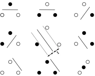
Figure 2.5: In a two dimensional space a maximum of three points can be completely shattered by a plane.

sucient condition for convergence in the context of classication problems is

lim l→∞

(lnN(H, l))

l = 0, ∀ >0 (2.8)

The shattering coecientNis a capacity measure ofHfor classication problems, it denes the maximum number of dierent separations that can be obtained using the functions of H. Given l instances, the shattering coecient is at maximum 2l

since every point can be labeled in 2 ways. The meaning of equation 2.8 is, that if H is so rich, that the number of correct separations grows exponentially in l no learning takes place. In this case a hypothesishwhich explains the training set fully without any error can always be found.

Based on the shattering coecient, Vapnik and Chervonenkis introduced another capacity measure, the VC-Dimension. It is dened as the maximum sample size l which can be completely shattered by H

V C(H) = max l|N(H, l) = 2l

(2.9) As we see the VC-dimension is a worst case measure, if h can shatter all points inS than no learning takes place. If all points are shattered byh it is impossible to determine if his a good model based on the training set. Because it is not possible to nd an instance xi ∈ S which could show that h(xi) 6= yi is a bad model. The

VC-dimension is, as well as the shattering coecient, independent of the underlying distribution of the samples which are shattered. The example in gure 2.5 shows a classier with VC-Dimension 3 which can shatter three points. A VC-dimension of 3 does however not mean that all sets of size 3 can be shattered, as shown in the example at the bottom right. For the gure in the middle we have shown a special case, the plane separating the two classes of points is situated such that the distance

(18)

0 20 40 60 80 100 0 5 10 15 VC−dimension VC bound

Figure 2.6: The value of the VC bound depending on the VC dimension ofH for l = 100

andδ = 0.1.

to the nearest points is equal. This kind of separation is called optimal separating hyperplane and it is the principle the support vector machines are built upon, as we will discuss later. In general the VC-dimension of a separating hyperplane in

RN upper bounded by V C(h) = N + 1 [20], so that the capacity of the classier

depends only on the number of points needed to dene the hyperplane.

One is of course not limited to the use of hyperplanes in order to shatter points. Bartlett et al. [2] show for example how to determine the VC-dimension of Neural Nets in order to determine the number of training points needed to achieve a good generalization of the network. It is important to point out that the VC dimension does not necessarily depend on the number of parameters used to specify h, for example the function h : _R → {+1,−1} = sign(sin (αx)) with one free parameter

is able to shatter innite points as shown in [6]. In addition to the VC-dimension there are other capacity concepts dened in SLT such as entropy, annealed VC-entropy of the growth function which are more specic than the VC-dimension [19] and lead to stricter bounds but are more dicult to determine.

Let us now see how the capacity measure is linked to the generalization ability of a specic hypothesis. The expected risk of a hypothesis h which minimizes the empirical risk given an arbitrary training set ofl samples satises

R(hl)≤Remp(hl) + s 1 l d ln2l d + 1 + ln4 δ | {z } capacity term (2.10) with probability of at least 1−δ given the VC-dimensiond =V C(H)[20]. This

(19)

d is also called capacity term as referred to by [20],[24].

2.2.4 Structural Risk Minimization

In order to complete our discussion about SLT, let us now see how to selectH such that bound on the expected risk is minimized. The idea of structural risk mini-mization (SRM) is to reduce the bound dened by 2.10 by minimizing the empirical error and the capacity term simultaneously. Vapnik proposes to use a hypothesis class H = H1 ⊂ H2. . . ⊂Hn which is composed of nested subsets with nite VC-dimension and choose thehl from the set H which minimizes 2.10. Referring to the

regression example shown in gure 2.4 this means to interpolate with polynomials of dierent degree and choose the h such that the approximation error as well as the capacity term is minimized simultaneously. SRM is useful especially in cases where the number of training samples is small and the empirical risk Remp is not

close to the actual risk R as pointed out by Vapnik in [23]. According to Hastie et al. [15] the main challenge in order to apply SRM is to determine the VC-dimension

H accurately, they state that it is usually only possible to obtain upper bounds on the VC-dimension. Burges noted in [6] that the VC bounds for a support vector machine are very loose depending on the used kernel, but are predictive enough to choose a specic classier h.

2.3 Optimization Theory

As we have seen in the last section solving the learning problem using empirical risk minimization is an optimization problem. Before we continue and show how this problem is solved using the support vector machine approach, we introduce a math-ematical optimization method. The method of Lagrange multipliers describes how a function can be minimized subject to a number of constraints. In our description we follow the denitions given by Boyd in [5]. The optimization problem, also referred to as the primal problem, is solved by Lagrange multipliers is dened as

arg min f0(x)

subject to fi ≤0i= 1. . . M

hi = 0i= 1. . . P

(2.11) By introducing the Lagrange multipliers α and β the inequality and equality constraints are included in the optimization problem leading to the LagrangianL

(20)

L(x, α, β) = f0(x) + M X i=1 αifi(x) + M X i=1 βihi(x) (2.12)

We assume that the DomainDof the problem is nonempty, such that an optimal valuep∗ can be found.

2.3.1 Lagrangian Duality

Let us now see how the optimal value of p∗ can be found. For every Lagrangian L we can dene a dual function

g(α, β) =min

x L(x, α, β) (2.13)

As shown by Boyd the dual function is a lower bound on the optimal solution p∗ and the following holds for every feasible pointx˜

g(α, β) =min

x L(x, α, β)≤L(˜x, α, β)≤f0(˜x) (2.14)

In order nd a nontrivial solution it is necessary to restrict α ≥ 0 otherwise we

could choose the Lagrange multiplier such that g(α, β) = −inf at each feasible

point. The Lagrange multiplier β does not need to be positive, since the value of hi(˜x)for a feasible point is zero as given by the constraint. In order to nd the best

value of the dual function, that is the lower bound which is the closest to p∗, the following optimization problem must therefore be solved

max

α, β minx L(x, α, β)

subject to α ≥0

(2.15) This problem is referred to as the Lagrange dual problem. Let us now state the conditions under which the optimal solution d∗ to the dual problem is equal to the optimal solution p∗ of the primal problem. If the condition d∗ = p∗ hold, then the bound obtained from the Lagrangian dual is tight [5] and we speak of strong duality. One constraint under which strict duality holds is Slaters condition[5]. Given that the primal problem of the form

min

x f0(x)

subject to fi ≤0, i= 1. . . M

Ax =b

(2.16) it states that there must exist an x in the relative interior of D such that the inequality conditions fi are strictly satised. In other words for all inequality

(21)

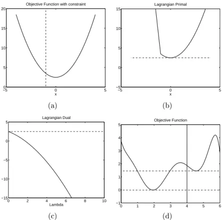
con-−50 0 5 5 10 15 x (a) −5 0 5 −5 0 5 10 x (b) 0 2 4 6 8 10 −15 −10 −5 0 5 Lambda Lagrangian Dual (c) 0 1 2 3 4 5 6 −1 0 1 2 3 4 5 Objective Function (d)

Figure 2.7: The primal and dual solution for a convex (a) and a non-convex optimization problem (d)

straints fi the following holds fi(x)<0. If we further restrict the problem

assum-ing that hi is ane and fi and f0 are convex, the Karush-Kuhn-Tucker conditions (KKT) are sucient for strong duality. For a convex optimization problem the KKT conditions are dened as

fi(˜x)≤0 primal constraint, i= 1. . . M

hi(˜x) = 0 primal constraint, i= 1. . . P ˜

αi ≥0 dual constraint ˜

αifi(˜x) = 0 complementary slackness condition ∇xf0(˜x) + X i ˜ αi∇xfi(˜x) + X i ˜ βi∇xhi(˜x) = 0

rst order derivatives of the primal must vanish for x˜

(2.17) If the KKT conditions hold for at a point x˜, α˜, β˜ then this point is primal and dual optimal.

The equivalence of the primal and dual solution is shown in gure 2.7 (a) - (c). We see how the minimum of the function f(x) =x2+ 2.5 subject to the constraint

(22)

the maximum of the dual is alsod∗ = 2.5, both values are equal since the constraint

function and the objective function are convex. In gure 2.7(d) a non-convex func-tion f0 is minimized subject to the convex constraint −x <= 4, the horizontal lines indicate p∗ and d∗. Using the dual formulation in order to solve this problem we fail to nd the correct minimum subject to the constraint leading to a duality gap between the primal and the dual solution.

In this section we have shown how optimization problems can be solved subject to a number of constraints. We have seen that for a particular type of optimiza-tion problem, namely a convex problem with convex inequality and ane equality constraints, it is possible to solve the Lagrangian dual (2.15) and obtain the same solution as if the Lagrangian primal (2.14) is solved. Up until now there is no reason why we should prefer to solve the optimization problem in the dual form, but as we will see shortly the dual formulation and especially the complementary slackness condition of KKT have very interesting consequences.

2.4 Support Vector Machines

The former sections described the Statistical Learning Theory and a mathematical method to solve a specic kind of optimization problem, this section shows how those theoretical concepts are applied in order to build a well generalizing non-probabilistic classier. This algorithm is the support vector machine, it is based on the minimization capacity term with respect to the empirical risk in order to minimize the expected risk.

2.4.1 Hard-margin SVM

The hard margin support vector machine, is a classier which assigns the labelyi to

xi based on the distancef(xi)of the instance to a decision boundary. The simplest

way to separate points is by a hyperplane, by classifying an instancexaccording to

its distance from the hyperplane dened by vector w and osetb

h(x,w, b) =θ wTx+b. (2.18)

That function θ represents an indicator function whether or not the distance is positive or negative. In order to nd a solution to the above problem, that is to nd w and b which dene the hyperplane, the training set S needs to be linearly separable. That is all points of a class are situated on the same side of the hyperplane, satisfying the following inequality

yi wTxi+b

(23)

if the following holds for all training examples yi

wT_x₊_b

||w|| ≥γ (2.19)

As we have see in equation 2.10 from section 2.2 the expected risk is bounded by the empirical risk and the capacity of the the hypothesis classH. In case of the problem of nding the optimal separating hyperplane for a linear separable problem, minimizing the expected risk 2.10 reduces to the minimization of the capacity term. This is because the empirical risk of misclassifying a linearly separable dataset using a separating hyperplane is zero. As already stated the VC-dimension of a hyper-plane is independent of the number of training points l and only inuenced by the dimensionality of x. We stated previously that the VC dimension is in that case

N + 1 if x ∈ _RN. This bound can be rened as shown by Vapnik [23]. Given

training instances from an N-dimensional x and belonging to a sphere of radius R the VC-dimension of thisγ-margin separating hyperplane is

V C(h(x,w, b)) =min R2 γ2, d + 1 (2.20)

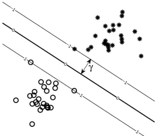
Following the principles of SRM the optimal separating hyperplane from the hyperplane which separates the training set without error, is the one which has the smallest VC-dimension. Or in other words the hyperplane which separates both classes in such a way that the distance from the instances to the hyperplane is maximized simultaneously for both classes as shown in gure 2.8. From the above equation we see that this is condition is fullled for the separating hyperplane with the largest geometrical margin γ such that all points are classied correctly. According to the SLT the VC-dimension is dened as a capacity measure for a function class H with the denition of the VC-dimension given in equation 2.20 it is now possible to evaluate the capacity for a specic functionh. That is nding the optimal separating hyperplane corresponds to the following optimization problem

h(x,w, b)∗ = max w,b γ subject to yi wTxi+b ||w|| ≥γ , i= 1. . . M

Let us now express the geometrical margin γ in terms of the functional margin

ˆ γ =;y wT_x₊_b h(x,w, b)∗ = max w,b ˆ γ ||w|| subject to yi wTxi+b ≥ˆγ , i= 1. . . M

(24)

0 0 0 1 1 1 −1 −1 −1 γ

Figure 2.8: The optimal separating hyperplane

Using the fact that we can always scale wand b by a constant without changing the geometrical margin, we can replace γˆ by 1. The optimization problem now

simplies to h(x,w, b)∗ = max w,b 1 ||w|| subject to yi wTxi+b ≥1, i= 1. . . M

which is equivalent to the following quadratic optimization problem [23] h(x,w, b)∗ = min w,b 1 2||w|| 2 subject to yi wTxi+b ≥1, i= 1. . . M (2.21) In order to solve this convex quadratic optimization problem given the inequality constraint yi wTxi+b

≥ 1, the method of Lagrange multipliers is used. The

Lagrangian of equation 2.21 is dened as

LP(w, b,α) = 1 2w T w−X i αi yi wTxi+b −1 subject to αi ≥0

The optimal separating hyperplane or in other words the hypothesish∗ with the smallest bound on the expected error is found by minimizing the Lagrangian with respect tow, b and maximizing it with respect to α.

(25)

h(x,w, b) = min

w,b maxα LP (w, b,α)

subject to αi ≥0

(2.22) This problem is the primal optimization problem, as we can see it corresponds to solving the empirical risk minimization problem regularized by the capacity of the separating hyperplane. Since both the primal problem of minimizing 1

2||w|| 2 _and the constraints are convex, we can equally solve the corresponding dual problem

h(x,w, b)∗ = max

α minw,b LP (w, b,α)

subject to αi ≥0

(2.23) In order to minimize the dual with respect tow, b let us take the derivative and set it to zero LP ∂w =w− X i αiyixi w=X i αiyixi LP ∂b =− X i αiyi 0 = X i αiyi (2.24)

Substituting the above results into equation 2.23 we obtain the so called Wolfe dual. LD =max α X i αi− 1 2 X i X j αiαjyiyjxTi xj subject to X i αiyi = 0, αi >0 (2.25) After nding the values for α∗_i by applying an algorithm to solve this problem, we need to determine the optimal value for the oset b since it is excluded from the dual solution. We know that the KKT conditions need to be satised in order to make α∗_i optimal in the sense of zero duality gap, therefore we can exploit the complementary slackness conditions. We ndb such thatαi yi wTxi+b

−1

= 0

is satised for all xi with αi = 0. In order to ensure numerical stability, Burges([6])

points out to take the mean value of allb resulting from the single equations. Once the optimal separating hyperplane is dened by determiningwand b we are able to classify a previously unseen instance x by evaluatingwT_x₊_b _{in the following way}

(26)

h(x,w, b) =sgn wTx+b =sgn   X i αiyixi !T x+b   =sgn X i αiyixTi x+b ! (2.26)

Let us now characterize the properties of the solution. The classication of x

depends on the linear expansion of w in terms of the training points xi. This

ex-pansion is sparse, this follows from the complementary slackness condition. Only those points whereyixTi w+b = 1 have a weightαi >0, since the value ofαi can be

maximized without violating the complementary slackness condition. Those points are referred to as support vectors and the algorithm solving for the optimal sepa-rating hyperplane by maximizing the margin is called hard-margin support vector machine. In gure 2.8 we see that only three points have a functional margin of 1, those points dene the optimal separating hyperplane. All other points of the training set are not taken into account when dening the decision boundary.

The advantage of the hard-margin support vector machine over other classiers such as Neural Networks is that the optimization problem has a unique solution, the learning process is rather fast and by constructing the decision rule one obtains a set of support vectors [23]. We refer to unique solution in the sense, that there is one hyperplane which separates the two classes in the best possible way and that any solution found for equation 2.23 is a global minimum. Furthermore using the SVM allows for training with small sample sizes in cases where the empirical risk minimization does not guarantee a small value of the expected risk R, due to the fact that the optimization objective is to minimize the capacity term.

The disadvantage of the hard-margin support vector machine is that it is dened for linearly separable datasets, which is a strong assumption and limits the applica-bility of the classier to real-world data sets. There are two principle ways to deal with the problem of linearly non-separable datasets, either to map the data into a higher dimension where the data is linear separable or to formulate the problem so that a certain amount of misclassication is tolerated. The former approach is called the kernel trick and leads to a non-linear decision surface in the feature space, the later one is the soft-margin support vector machine, both methods are usually combined. We will discuss both of them in the following sections.

(27)

0 0 0 1 1 1 −1 −1 −1 (a) 0 0 0 1 1 1 1 1 1 free S V margin violator, bounded S V (b)

Figure 2.9: Soft-margin SVM using a linear kernel, (b) shows the support vectors which dene the hyperplane

2.4.2 Soft-margin SVM

Since linear separability of two classes can not always be assumed, slack variables ξi were introduced by Cortes and Vapnik [11] in order to relax the separability

condition of the hard-margin SVM. A value of ξ > 0 is assigned to all points that

are situated either on the wrong side of the hyperplane or inside the functional margin wT_x ₊_b _≤ ₁_{. Consequently the optimization problem in equation 2.21}

is relaxed in such a way that margin violation is accepted φ(ξ) = PM

i=1ξi. All points for which0≤ξi ≤1holds, are situated on the correct side of the hyperplane,

whereas allξi >1are misclassied since they lie on the wrong side of the hyperplane.

Additionally to the slack variable the cost parameter C is introduced in order to balance the two optimization objectives to minimize wT_w _{and to ensure that the}

number of margin violators is small. min w 1 2w T w+CX i ξi subject to yi wTxi+b ≥1−ξi ξi ≥0 (2.27)

This constrained convex quadratic optimization problem can also be expressed in an unconstrained way introducing the hinge loss function

Lhinge yi,wTxi+b =max 0,1−yi,wTxi+b min w 1 2w T_w₊_CX i Lhinge yi,wTxi+b (2.28)

The loss function allows us to easily examine how margin violators contribute to the minimization problem and is a way to increase the robustness of the support

(28)

vector machine, as we will see later. This unconstrained optimization problem can be used by applying quadratic solvers or Newton type algorithms. However, the standard formulation of the soft-margin SVM algorithm uses the Lagrange multiplier method to solve the constrained optimization problem in the following way.

The Lagrangian of equation is dened as

LP = 1 2w T_w₊_CX i ξi− X i αi yi xTw+b +ξi−1 −X i µiξi subject to αi ≥0, µi ≥0 (2.29) In order to maximize it with respect to αi set its derivatives with respect to w,

b and ξi to zero LP ∂w =w− X i αiyixi LP ∂b =− X i αiyi LP ∂ξi =C−αi−µi w0 = X i αiyixi 0 = X i αiyi 0≤αi ≤C (2.30)

Finally we nd the corresponding dual as

LD =max α X i αi− 1 2 X i X j αiαjyiyjxTi xj subject to 0≤αi ≤C (2.31) Obviously equation 3.13 is very similar to the solution we found for the hard-margin SVM 2.23 except that the Lagrange multiplierαi is not unbounded anymore,

but upper bounded byC. It must satisfy the box constraints0≤α ≤C. Therefore we can distinguish between two dierent kinds of support vectors, all points which satisfy 0< αi < C are free support vectors, those points are margin violators with 0< ξ <1which are situated at the correct side of the hyperplane. All points which

are situated on the wrong side of the hyperplane are characterized by ξ > 1 and

αi =C, those points are also called bounded support vectors. This type of support

(29)

As we have seen in the last section one approach to deal with data which is not linearly separable is to tolerate a certain amount of misclassication. However the relaxation of the constraint in equation 2.21 does not decrease the bound on the expected risk. The idea of the nonlinear SVM is to map the data from the original feature spacex∈X to a higher dimensional space Zwhere it its linearly separable,

or where at least the margin is increased. The linear decision boundary in this high dimensional space corresponds to a nonlinear decision boundary in the original space. In that sense we incorporate an inductive bias, the knowledge that the data is linearly separable in the high dimensional space, in order to solve the classication problem. Letφ:X→Zbe such a mapping, and letZ be a space which is equipped

with an inner product, then we can rewrite the Lagrangian dual 3.13 as

LD =max α X i αi− 1 2 X i X j αiαjyiyjφ(xi)T φ(xj) subject to 0≤αi ≤C (2.32) However solving would be computationally complex, since it requires to evaluate the inner product in the high-dimensional spaceZ. Therefore kernels are introduced. A kernel is a function which evaluates the inner productφ(xi)

T

φ(xj)in the original

feature space Xsuch that

K(xi,xj) =φ(xi) T

φ(xj) (2.33)

The kernel can be interpreted as a function which measures the similarity measure between two points xi,xj. Therefore the usual approach is to dene a similarity

function K for a given problem such that it fullls the properties of a kernel and not to dene a high dimensional feature space and determine the kernel function afterwards. One criterion in order for a function K : X×X → _R to be a kernel is

that all nite kernel matrices must be positive semidenite. A good overview how to select, construct kernels and combine kernels can be found in [12].

In the following some popular kernels functions are listed, apart from the linear classier which uses no kernel, the radial basis function (RBF) kernel is the most used kernel in practice [21]. Note that the RBF kernel uses the same function as the Parzen based classier, however a Parzen window estimator does not yield the same results since it evaluates the kernel at all training points dierent from the SVM which only evaluates the kernel values of the support vectors.

(30)

0 0 0 0 0 0 0 (a) 0 0 0 0 0 0 0 (b)

Figure 2.10: Non-linear soft-margin SVM using a RBF kernel, (b) shows the support vectors which dene the hyperplane

K(xi,xj) = hxi,xji=xTi xj Linear Kernel K(xi,xj) = (hxi,xji+ 1)p Polynomial Kernel K(xi,xj) = exp −kxi−xjk 2σ2 RBF Kernel (2.34) Figure 2.10 shows the nonlinear decision boundary of a SVM induced by using the RBF kernel. The RBF kernel evaluates the Euclidean distance from a point to a support vectors due to this the shape of the decision boundary at a single point is circular or elliptic, as visualized at the top of the gure. By weighting with αi and

linearly combining the response of the kernel for all support vectors, the nonlinear decision boundary is formed.

2.4.4 Robustness of the SVM

The robustness of support vector machines was studied by Steinwart and Christ-mann in [21] and more general with regard to the robustness properties of convex minimization methods in [9]. More recently Hable and Christmann [14] studied the qualitative robustness of support vector machines. Xu et al. [27] also studied the robustness properties of the SVM and showed that the standard support vector machine solution is equivalent to the solution of a robust optimization problem.

Steinwart applies methods of robust statistics to derive conditions under which non-linear soft-margin support vector machines are robust. He analyzes how changes in the distribution of the random variablesX and Y aect the classier's accuracy depending on the loss function, kernel used and cost parameter C. Steinwart uses

(31)

vector machines. An inuence function measures the impact of a small amount of contamination of the original distributionP of X and Y in the direction of a point z on the quantity of interest [21]. In other words it evaluates how the accuracy of the classier changes if the data used for training is contamined by noise. Based on the theoretical analysis Steinwart concludes that if the rst derivative of a convex margin-based loss function is bounded and a bounded continuous kernel is used, then the inuence function of the SVM is bounded. That is the standard SVM using the hinge loss function in combination with a bounded kernel, as for example the RBF kernel, has a good statistical robustness property. Furthermore Steinwart shows that the robustness of a SVM can be increased by choosing a small value of C.

(32)

3. ROBUST SVM APPROACHES

After introducing the theoretical background of support vector machines in the last chapter, we now discuss the dierent approaches that have been proposed to improve the robustness of the SVM algorithm against outliers by using loss functions dier-ent than the hinge loss. The aim of using alternative loss functions is to make the classier robust against outliers, dierent from those approaches who lter the train-ing data before traintrain-ing the nal classier. The approach of maktrain-ing the classier robust against outliers is attractive because explicit ltering is usually computation-ally complex since it is either based on the estimation of the data distribution or on the construction of new features. An example of a robust SVM formulation which is based on explicit ltering is the weighted support vector machine proposed by Yang et al. [29]. They propose to apply the kernel-based possible c-means algorithm as a preprocessing step in order to weight each training instance according to its eu-clidean distance from the cluster centers. In the following we present the dierent approaches which rely on implicit outlier ltering by using a modied loss function.

3.1 The Inuence of the Loss Function on the SVM

Before we start and show what kind of dierent loss functions for SVMs have been proposed and how the optimization problems are solved, we rst show how the loss function inuences the decision boundary following the discussion of Chapelle [8]. The unconstrained optimization problem of a soft-margin support vector machine with an arbitrary loss function is given as

min w 1 2w T_w₊_CX i L yi,wTxi+b . _(3.1)

If we drop the oset term b and set f(xi) = wTxi, we can simplify rewrite the

problem as min w 1 2w T_w₊_CX i L(yi, f(xi)). (3.2)

We dierentiate the above equation with respect to w and set the derivative to

(33)

−2 −1.5 −1 −0.5 0 0.5 1 1.5 2 0 0.5 1 1.5 y_if(x_i) Loss

Zero−One loss

−2 −1.5 −1 −0.5 0 0.5 1 1.5 2 0 0.5 1 1.5 y_if(x_i) Loss η_0.1 η_0.5 η 0.9 −2 −1.5 −1 −0.5 0 0.5 1 1.5 2 −1 −0.5 0 0.5 1 1.5 2 2.5 3 y_if(x_i) L o s s C onvex part C oncave part Truncated hinge loss

s −2 −1.5 −1 −0.5 0 0.5 1 1.5 2 0 0.5 1 1.5 2 y_if(x_i) Loss

Gaussian error function

Figure 3.1: Four dierent loss functions

w+CX i ∂L(yi, f(xi)) ∂w = 0 w+CX i ∂L(yi, f(xi)) ∂f(xi) f(xi) ∂w = 0 w+CX i ∂L(yi, f(xi)) ∂f(xi) | {z } βi xi = 0. (3.3)

From the above equation we see that w can be written as a linear combination

of training instancesxi. Equation 3.3 directly shows that the inuence of a training

instance xi on the decision boundary dened by w depends on the loss function

used. Each training instance xi is weighted by the derivative of the loss function

with respect tof(xi). Thus instances which are located in a at area of L have no inuence on the expansion of w. This is because including them in the expansion

would not reduce the objective value of equation 3.1.

The hinge loss used in the standard SVM formulation is linear, that means all margin violators with yif(xi) < 1 contribute with the same weight C to w. This

(34)

means the larger the loss of xi the more benecial is it to include the point in

the expansion of w. This is indeed the same result as we achieved by solving the

soft-margin support vector machine in the dual. From the complementary slackness condition we know, that only the margin violator contribute with 0 < yiαi < C to

the expansion of w.

Therefore the aim of the robust SVM methods is to use loss functions which have at regions for points whose distance from the decision boundary yif(xi) is very

large and can be regarded as outliers. Eectively the loss functions are non-convex which makes it necessary to use other optimization methods than in the standard SVM formulation. In the following we will discuss the robust SVM approaches based on the loss functions shown in gure 3.1.

3.2 η

-Hinge Loss Function

Along with a ltering approach Xu et. al [28] present the η-hinge loss. They bound the inuence on outliers by minimizing the SVM optimization problem over a set of loss functions. The corresponding robust eta loss function is dened as

Lη(yi, f(xi)) = ηi[(1−yif(xi) +b)]₊+ 1−ηi (3.4)

with f(xi) = wTxi +b. The value of ηi is bounded to by 0 ≤ ηi ≤ 1 and all

training instances xi which can be regarded as outliers will be assigned a value of

ηi = 1. All other instances are assigned ηi = 0. The eect of setting ηi to 1 for all

outliers is, that the corresponding loss function will be a constant. All instances xi

withLη(yi, f(xi))inside a constant region are ltered and will not become support

vectors. Therefore the optimization objective of the η-hinge loss is to minimize ηi.

The primal form of the optimization problem for the η-hinge loss is stated as min w minη 1 2w T_w₊_CX i η[(1−yif(xi) +b)]₊+ 1−η subject to 0≤ηi ≤1 (3.5) As pointed out by Xu minimizing the above equation by alternating the mini-mization ofwand η yields boolean solutions with ηi = 0 for all outliers and ηi = 1.

They state that this approach is prone to yield solutions which are local minima. Therefore they reformulate the problem in order to simultaneously optimize wand

(35)

min 0≤η≤1minw 2||w|| 2 ₊_C i ηi 1−yixiTw ++ 1−ηi =min 0≤η≤10≤maxα≤C η T ₍_α₋_e₎₋1 2α T _YXT_XY_◦_ηηT α+t withG=YXTXY = min 0≤η≤1, M=ηηT 0≤maxα≤C η T ₍_α₋_e₎₋ 1 2α T ₍_G_◦_M₎_α withM ηηT =M −ηηT 0 = min 0≤η≤1, MηηT _0≤max_α_≤_C η T ₍_α₋_e₎₋ 1 2α T ₍_G_◦_M₎_α (3.6)

This problem is a convex optimization problem, however the optimization variable M is not a vector but a positive semidenite matrix, such kind of problems are solved by quadratic-programming solvers. Xu mentions that the proposed method is robust, but that it is not possible to identify outliers by evaluating the values of ηi after solving the optimization problem. Therefore Xu proposes to drop the

term 1−η in formula 3.5 such that ηi serves as a weight factor for each training

instancexi yielding the robust outlier detection algorithm. A similar approach has

been applied by Zhou et al. [30] and will be explained later.

3.3 Truncated Hinge Loss Function

The truncated hinge loss function is an alternative way to dene a robust loss func-tion and is usually implemented by combining two hinge loss funcfunc-tions as shown in gure 3.1(c). It was rst applied to the support vector machine by Collobert et al. [10] in the context of transductive SVMs in order to reduce the number of support vectors by removing errors from the training set. Wu et al. [26] extend the approach by Collobert to multiclass support vector machines. Wang et al. [25] on the other hand combine two Huber loss functions so that the edges of the truncated hinge loss function are smoothed. All three approaches use the constrained concave-convex procedure (CCCP) to solve the optimization problem as described in equation 3.8. Assuming that the objection functionJ(w)can be split into a convex partJvex(w)

and a concave part Jcave(w), the CCCP minimizes the objective function J(w) in

an iterative way as shown in algorithm 1.

The optimization problem based on the truncated hinge loss function is then stated as a dierence between two hinge loss functions H1 and Hs.

min w 1 2w T_w₊_CX i H1(yif(xi)) | {z } Jvex(w) −CX i Hs(yif(xi)) | {z } Jcav(w) (3.8)

(36)

Algorithm 1 CCCP algorithm Initialize w0 repeat wt+1 =min w Jvex(w) +J 0 cave(w)·w (3.7) until convergence of wt

Collobert as well as Wu solve the optimization problem stated in equation 3.8 by applying CCCP as shown in algorithm 2.

Algorithm 2 CCCP for solving the ramp loss problem β0 = 0

repeat

Solve the convex optimization problem max α X i αi− 1 2 X i X j αiαjyiyjxTi xj subject to −β_it−1 ≤αi ≤C−βit−1 X i yiαi = 0 (3.9)

Compute bt using the unbounded support vectors 0< αt_i < C ⇒yif(xi) = 1

Update β_it= ( C yif(xi)< s 0 otherwise (3.10) until βt=βt−1

The advantage of solving this problem in the dual is, that standard SVM solvers can be used to solve the convex problem. Collobert proposes to train the initial clas-sier withβi = 0 on a subset of the training data. This corresponds to the standard

training procedure based on the hinge loss function. Based on this initial classier all points which have a distance from the margin larger than s will be removed by setting βi = C and thus consequently setting αi = 0 in the next convex training

step. Wu applies CCCP in the primal in order to solve the optimization problem with a Newton-type algorithm and setsβi = 0 in equation 3.3 for those points who

(37)

−2 −1.5 −1 −0.5 0 0.5 1 1.5 2 0 0.5 1 1.5 y if(xi) L o s s s

Figure 3.2: The ltering hinge loss function

3.4 Integrated Outlier Filtering

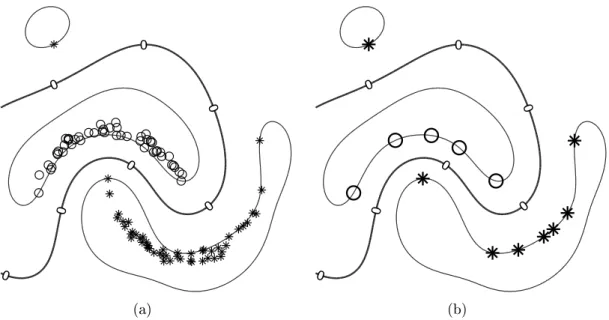
The integrated outlier ltering approach by Zhou [30] is an implementation of the robust outlier detection method proposed by Xu et al. [28] using the loss function shown in Figure 3.2. In order to show the equivalence we continue to use the notation introduced in section 3.2. The optimization problem is stated as

min w ηimin∈{0,1} 1 2w T_w₋X i ηiξi subject to X i ηi ≥M (3.11) where ηi is a binary ltering variable and M the number of non-outliers in the

training set. This problem is then transformed into a semidenite program by relaxing the binary constraint on η to0≤ηi ≤1, as shown above

min 0≤η≤1minw 1 2||w|| 2 +CX i ηi 1−yixiTw + =min 0≤η≤10≤maxα≤C η T (α)− 1 2α T YXTXY◦ηηTα subject to 0≤αi ≤C, eTη≥M G=YXTXY = min 0≤η≤1, MηηT max_α η T ₍_α₋_e₎₋ 1 2α T ₍_G_◦_M₎_α subject to 0≤αi ≤C, eTη≥M (3.12)

In addition to this approach, which Zhou refers to as semi-denite programming robust SVM, Zhou proposes a multi-stage relaxation of the semi-denite program-ming based formulation based on CCCP as shown in Algorithm 3.

The Multi-stage robust SVM algorithm trains a support vector machine itera-tively and removes outliers during each iteration. Since the derivative of the loss

(38)

Algorithm 3 Multi stage relaxation of integrated outlier ltering η0 =1

repeat

Solve the convex optimization problem

Lt_D =max α X i αi− 1 2 X i X j ηiαiαjyiyjxTi xj subject to 0≤αi ≤C (3.13) Update, sortui =yif(xi)in ascending order

η_it= ( 0 if the rank ofui > M 1 otherwise (3.14) until Lt_D−1 −Lt D is suciently small

function of this algorithm is equal to the derivative of the truncated hinge loss dis-cussed in section 3.3 both approaches are equal. This can also be seen by analyzing the algorithms. Settingηi = 0in algorithm3has the same eect as choosingβi =C

in algorithm 2. Both approaches dier only in how they identify outliers. Zhou assumes that the number of non-outliers M is known beforehand and removes the outliers according to their rank, whereas Wu uses a threshold on the distance to the margin in order to identify outliers. Another dierence is that the iterative removal of outliers according to their rank converges afterM instances are left in the training set, the threshold criteria of the truncated hinge loss however only removes points according to the specied threshold.

(39)

4. EXPERIMENTS

The dierent methods to make support vector machine robust against noise by us-ing modied loss functions were introduced in the last chapter. In this chapter the performance of the methods based on the truncated hinge loss function which solve the optimization problem in the dual is analyzed. The motivation to analyze this type of approaches is that they can be easily adopted to highly ecient SVM solvers as LibSVM. The approaches based on the truncated hinge loss function proposed by Collobert [10] and the Integrated outlier ltering for large margin training pro-posed by Zhou [30] fulll this requirement. Collobert removes all training instances with a distance to the margin greater than a xed value, Wu which implements the same approach in the primal proposes s = −1 as a threshold. Zhou on the other

hand removes a certain percentage of the largest margin violators and states that the optimal amount of outliers to remove can be estimated by cross-validation.We will refer to the two approaches in the following as threshold ltering and rank l-tering in our tables and plots. Both methods use the truncated hinge loss function in order to remove outliers.

The objective of our experiments is to determine if the classication accuracy of the robust methods is higher than the accuracy of a standard support vector machine in the presence of noise during training. Furthermore we want to examine if it is possible to determine the optimal robustness parameter for both methods by applying cross-validation as stated by Zhou [30]. The experimental study is de-signed according to the guidelines for machine learning experiments described by Alpaydin [1]. Following those recommendations we now give an overview over the central points of the experimental study.

We test the hypothesis that the robust algorithms perform better than the stan-dard support vector machine in the presence of noise. The primary response variable used to test the hypothesis is the classication accuracy of the dierent algorithms on noisy data sets which we acquire in our experiments. Since the robust algorithms rely on implicit outlier detection and their removal, we also measure the accuracy of the outlier removal process using the F1-score as response variable. Furthermore the number of support vectors is selected as measure of the classiers complexity.

(40)

Data set Dimensionality #Training #Test

UCI Breast cancer 10 383 95

UCI Diabetes 8 429 108

UCI Ionosphere 34 202 50

UCI Liver disorders 6 236 58

UCI Fourclass 2 492 122

UCI Heart 13 192 48

UCI Sonar 60 156 38

Table 4.1: Dimensionality and size of the training and test sets used for evaluation

The support vector machines, and therefore the response variables, are generally inuenced by a variety of factors. The controllable factors of our study are the cost parameter C of the soft-margin SVM, the parameter for the RBF kernel and the robustness parameter controlling the removal of outliers. The scale of the features and the ratio between the number of samples per class are also well known factors [3] [16] which aect the performance of support vector machines. In the following we describe the data sets used, how they are are preprocessed and resampled as well as the experimental strategy used to address the controllable factors.

4.1 Data sets, Resampling and Preparation

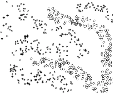
Seven dierent data sets representing binary classication problems are selected for the evaluation of the algorithms, their main characteristics are shown in table 4.1. The data sets are provided by the UCI machine learning database [13] and were retrieved from the collection of data sets provided at the LibSVM website [17]. The UCI data sets are widely used in publications and can be considered as standard evaluation data sets. The dimensionality as well as the size of the data sets selected is small to medium and all data sets are prone to noise. Figure 4.1 illustrates the distribution of the samples after applying t-Distributed Stochastic Neighbor Embedding as dimensionality reduction technique. As we can see from the gure, the two data sets UCI Breast cancer and UCI Fourclass are special since they are almost completely separable.

Regarding the data preparation it is necessary to scale each feature of the data sets such that they lie in the same interval as proposed by [16]. Since the data sets provided by the LibSVM website are standardized to a range of[−1,+1]no further

data preprocessing is applied.

The seven data sets selected are not divided into training and test sets, we there-fore apply a resampling in order to split the data into training and test sets. Bethere-fore dividing the data sets we stratify them such that both of the classes are represented by the same number of samples. The stratied data sets are then resampled by applying the ve-fold cross-validation method as proposed by [18]. We set the repli-cation number to 100 such that 500 training and test set pairs are generated for each UCI data set. Since we use ve-fold cross-validation 80% of the original data

(41)

(a) UCI Breast cancer (b) UCI Diabetes (c) UCI Ionosphere

(d) UCI Liver disorders (e) UCI Fourclass (f) UCI Heart

(g) UCI Sonar

(42)

set size is used for training and 20% for testing. For each of the 100 cross-validation sets consisting of ve training and test set pairs, the test sets are mutually exclusive. After collecting the response variables for each cross-validation set, we average their values yielding an overall number of 100 measurements.

In order to study how much the classication accuracy is aected by label noise, we generate 100 label noise realizations by randomly ipping 5% to 15% of the class labels for each data set as done in the experiments by Zhou. Additionally to random label noise we generate 100 instances of adversarial label noise. Dierent from ran-domly chosing the labels to ip we rst train a SVM on the unpolluted dataset and ip the labels of the instances of class 1 which have the maximum positive distance from the decision boundary. By doing so the instances with the ipped labels can be regarded as outliers with respect to class 2. After generating the noise realiza-tions we apply the same cross-validation method yielding 500 training and test set pairs for each noise level,data set and noise-type. We store all training and test sets generated in order to provide the dierent algorithms with the same training and test data following the blocking approach.

4.2 Experimental Strategy

By scaling and stratifying the data two inuencing factors are removed. The re-maining factors are the cost parameter C of the SVM, the parameter for the RBF kernel and the robustness parameter. In the following we describe how the best parameter combination is selected.

Determining the best cost-,kernel- and robustness parameters in terms of classier accuracy is costly. A commonly used method to determine the optimal parameter combination is the grid search which simply tests all combinations of parameters in a given range. A more sophisticated approach is unconstrained nonlinear optimiza-tion. It takes the value of the objective function into account when selecting the next combination of parameters subject to test. We compared the results of the grid search and nonlinear optimization in terms of computational complexity as well as accuracy and decided to use grid search.

As shown above the grid search tests all parameter combinations in a given range by training the classier on a training set and evaluating its performance on a validation set. For each run in our experiments we randomly select 20% of the

training data as a tuning set and apply 5-fold cross-validation during the gridsearch. That is ve dierent training and validation sets for the gridsearch are generated based on the tuning set. Once the optimal parameter conguration is found we train the nal classier on the whole training set and test its classication accuracy on the independent test.

(43)

for a RBF kernel.

for log2c=−5→7 do

for log2gamma=−7→5 do

do 5-fold cross-validation

if average accuracy over 5-fold cv ≥best accuracy found so far then

update optimal parameter set end if

end for end for

In order to determine if the optimal robustness parameter can be selected by grid search, we extend the above algorithm by an outer loop searching a specied range. For rank based ltering we select the range as s = 5−50%. This range

is much larger than the amount of added noise, since we do not want to introduce information leakage. By analyzing the optimal values we will be able to judge if the optimal parameters found are related to the noise added. For threshold based ltering we choose a range of [−1000,−2 : 0.5 : 0]. Setting the treshold value to −1000 corresponds to not removing any training instances, training instances at

s= 0 are situated directly at the decision boundary.

4.3 Implementation

Both robust support vector approaches are implemented in Matlab using the Matlab-Interface of LibSVM-Weights-3.12[7]. We choose the standard LibSVM 3.12 [7] im-plementation as the reference algorithm in our experiments. All tests are conducted on a Core i5 3.1 GHz computer with 8GB RAM, the statistical analysis is performed using the Statistical Toolbox of Matlab 2011b.

(44)

5. RESULTS

0.650 0.7 0.75 0.8 0.85 0.9 0.95 1 2 4 6 8 10 12 14 16 Accuracy Frequency 0.650 0.7 0.75 0.8 0.85 0.9 0.95 1 5 10 15 20 25 Accuracy Frequency 0.650 0.7 0.75 0.8 0.85 0.9 0.95 1 2 4 6 8 10 12 14 16 18 Accuracy Frequency 0.650 0.7 0.75 0.8 0.85 0.9 0.95 1 5 10 15 20 25 30 Accuracy Frequency 0.650 0.7 0.75 0.8 0.85 0.9 0.95 1 2 4 6 8 10 12 14 16 18 Accuracy Frequency

Figure 5.1: Histograms of the accuracy measures of the tested methods on the Ionosphere data set contamined by 10% label noise using a linear kernel.

After describing the experimental setup and strategy we will now discuss the re-sults of the experiments. We rst examine the distribution of classication accuracy measurements. Figure 5.1 shows the accuracy histograms of the dierent approaches tested. As we can see the accuracy values are situated in the same range, but their distributions dier.

In order to compare the measurement values, especially when their dierences are small, we apply a statistical signicance test to ensure that the dierences between the algorithms are meaningful. We choose the Wilcoxon signed-rank test with p <

0.05 as an non-parametric statistic signicance test. This paired dierence test

evaluates whether or not the dierence between the two series of measurements originate from a distribution with zero median. Due to the fact that we use the same training and test sets for each algorithm, we obtain paired samples and can therefore apply this type of test. All values reported are the median values of 100 measures. In the tables showing the accuracy values of the dierent approaches we print those values in boldface with p < 0.05.

We now present the individual results. We rst compare the results of the linear and the RBF kernel. Afterwards we compare the results for the robust methods with a xed robustness parameter and a cross-validated parameter. All measure-ment tables are attached in the appendix.

As we can see in gure 5.2(a) the reference LibSVM is only mildly aected by label noise given a linear kernel and a nearly linearly separable dataset like UCI Breast cancer. Without any outliers LibSVM yields an accuracy of 96,45% and