DOI 10.1007/s10898-007-9240-3
An algorithm for ordinal sorting based on ELECTRE
with categories defined by examples
Clara Rocha ·Luis C. Dias
Received: 11 September 2007 / Accepted: 13 September 2007 / Published online: 11 October 2007 © Springer Science+Business Media, LLC. 2007
Abstract This work proposes a Progressive Assisted Sorting Algorithm (PASA) based on a multicriteria evaluation ELECTRE-type method. The purpose of the PASA is to aid a decision maker to progressively sort a set of alternatives into a set of categories, which we considered are ordered (ordinal sorting), following a consistency principle. We consider the principle that if an alternative outranks (is as good as) a second one, then it must belong to the same category or to a better category. The set of alternatives already sorted by the decision maker will implicitly define the categories, and will constrain the range of catego-ries where other alternatives may be sorted. We show how the same idea may be used in an aggregation/disaggregation approach, considering some parameters of ELECTRE are not fixed a priori, but are constrained only by the examples provided. In this context, we establish a “convex-shape property” stating that the range of possible categories for an alternative is always an interval of categories. A discussion contrasting this approach with ELECTRE TRI is included in the conclusions.
Keywords Multi-criteria decision aiding·Sorting problem·ELECTRE·Aggregation/ disaggregation approaches
1 Introduction
Sorting problems are concerned with evaluating a set A of alternatives in order to assign them to mutually exclusive categories C1,C2, . . . ,Cncat. In multicriteria analysis, the assignment
C. Rocha
Escola Superior de Tecnologia da Saúde de Coimbra, Instituto Politécnico de Coimbra, Rua 5 de Outubro, S. Martinho do Bispo, Ap. 7006, Coimbra 3040-162, Portugal
C. Rocha
INESC Coimbra, R. Antero de Quental 199, Coimbra 3000-033, Portugal L. C. Dias (
B
)INESC Coimbra and Faculdade de Economia, Universidade de Coimbra, Av. Dias da Silva 165, Coimbra 3004-512, Portugal
of an alternative ai to a category results from its intrinsic evaluation on different criteria, as well as from the definition of the categories, sometimes also provided in terms of multiple criteria. Among the methods that have been proposed to handle multiple criteria sorting problems we can cite, e.g., Trichotomic Segmentation [12], N-TOMIC [11], ORCLASS [10], ELECTRE TRI [19], PROAFTN [1], UTADIS [21], a general class of filtering methods [17], rough sets [6] or the Koksalan-Ulu method [9].
In some cases, the categories are not ordered (nominal sorting or classification). For instance, one may sort the members of a database of persons offering themselves to work in a company into the categories “technical profile”, “commercial profile”, “leadership profile”, etc., without stating one category is the best or the most important. In other cases (ordinal sort-ing), the categories are ordered. For instance, one may sort the same job candidates into the categories “low potential”, “average potential”, “high potential”, etc., where the candidates placed in higher categories are supposedly better than the ones placed in lower categories. When the categories are not ordered, they are usually defined through prototypical elements (e.g., [1]), and the elements of A are sorted according to their similarity with such prototypes. When the categories are ordered, they can also be defined through prototypical elements, but typically they are defined through category limits, i.e., lower and upper bounds, where usually the upper bound of a category is the lower bound of the next better category (e.g., ELECTRE TRI [19]).
We are interested in ordinal sorting problems, with the categories ordered from worst (C1, by convention) to best (Cncat). For these problems, there have been some proposals based on aggregation/disaggregation approaches [3,8,21] to overcome the difficulties often felt by the Decision Maker (DM) when asked to provide values for the method’s parameters. In some of the best-known approaches, either based on utility functions [21] or based on ELECTRE TRI [3,14,16], the DM is asked to provide prototypical elements (i.e., sorting examples), although there exist parameters defining the category limits. In UTADIS [21], the examples are used to infer all of the method’s parameters, including the category limits; in ELECTRE, inferring all of the method’s parameters requires solving difficult non-linear problems [14]. As simplifica-tions, [3] assumes the category limits are given, whereas [16] addresses the difficult problem of inferring these limits from sorting examples. In all of these approaches, the examples are used to infer a sorting model, which may then be used to sort any other alternatives.
A different new direction consists in proposing ordinal sorting procedures without explic-itly defining category limits [5,9]. Rather, the DM is asked to sort some alternatives from
A as examples which will define the categories of the remaining alternatives. Doumpos and
Zopounidis [5] consider the examples as a learning set that can be used to define a sorting model based on the net flow of PROMETHEE, solving a linear program to minimize the violations of the classification rule. Koksalan and Ulu [9] propose an interactive procedure to help the DM add successively new examples until all the alternatives are sorted. Their interactive procedure, based on the additive aggregation model for multi-attribute utility functions, ensures the examples are provided in a consistent manner, namely, imposing the natural principle that if the utility of an alternative aiis equal to or higher than the utility of
aj, then the category of ai must be equal to or better than the category of aj.
The method of Koksalan and Ulu is to our knowledge a first example of what we call a PASA (Progressive Assisted Sorting Algorithm). The purpose of a PASA is to assist a DM in progressively sorting alternatives by assigning them to categories C1,C2, . . . ,Cncat. The DM exercises his or her judgement concerning each alternative to be sorted, with the aid of a PASA that constrains the categories where it may be placed if consistency is to be main-tained concerning previous judgements; namely, the DM is aided by learning the minimum and maximum category where an alternative might be sorted, given the examples already
sorted. Sometimes, the minimum and maximum will coincide. Otherwise, it is up to the DM to make a decision. In these cases, it is the DM who can assist the procedure by choosing one among an interval of potential categories for an alternative. This decision will in turn become a precedent for future ones. The spirit behind a PASA is hence that of aiding a DM to perform a series of sorting decisions in a consistent manner, rather than deriving a model to substitute the DM.
The purpose of this paper is to make a proposal of a PASA based on the ELECTRE methodology, rather than utility functions. However, unlike utility functions, there is not an undisputed principle of consistency to be followed, namely when we note that the outranking relation S defined by ELECTRE is not complete (alternatives that do not outrank each other are called incomparable), it is not transitive (e.g., aiSajand ajSak, but not aiSak), and it may present cycles (e.g., ajSakSaiSaj). These difficulties stem form the strengths of ELECTRE, namely the partial absence of compensation among criteria (a very low performance on one criterion may not be compensated by an excellent performance on another criterion) and the identification of incomparability (an alternative may not be sorted into a precise category because it is too different from any category limits or prototypes).
In this paper we put forward the suggestion (also advocated by [2]) of using the semantic meaning of the outranking relation (aiSaj means ai is at least as good as aj, i.e., ai is not worse than aj) to define a consistency principle: “if an alternative outranks a second one, then it must belong to the same category or to a better category”. Although seemingly logical and weak, this is a relatively strong requirement. For instance, it is not imposed by the ELECTRE TRI method. Let us note that the word consistency in this work refers to not contradicting the principle when outranking relations are used. Hence, lack of consistency may be due to misjudgments of the DM (i.e., judgements the DM is willing to change in retrospect), or may be due to the inadequacy of the principle, or may be due to the way the outranking relation is defined in ELECTRE.
This paper also proposes how the same procedure may be used even when not all of the method’s parameters have been fixed, using an aggregation/disaggregation approach. More concretely, we will assume that the criteria weights and the cutting level of ELECTRE have not been defined and will compute, for each potential sorting decision, a vector of weights and an interval of values for the cutting level that make the decision compatible with the previous ones. Therefore, we may conclude that there is more than one possible category for a given alternative because either it is incomparable to those already sorted, or because of the accepted variability of the weights and the cutting level, or for both of these reasons at the same time. We will consider the parameters that do not interrelate the criteria (i.e., the thresholds associated to each criterion individually) as fixed.
This paper is structured as follows. The next section briefly reminds how the [0,1]-valued outranking relation used by ELECTRE TRI is defined. Section3presents an ELECTRE-type PASA without explicit category limits, assuming all of the method’s parameters are fixed beforehand. Section4presents the same procedure in the context of an aggregation/dis-aggregation approach where the weights and the cutting level do not need to be precisely fixed. Section5presents two illustrative examples. Finally, in Sect.6we highlight the main characteristics of the proposed approach, discussing how it compares with ELECTRE TRI.
2 Valued outranking relations in ELECTRE
Let A= {a1, . . . ,am}denote a set of alternatives (actions, objects, projects) represented by a vector of evaluations on n criteria. Let g1(.), . . . ,gn(.)denote the set of criteria functions,
such that gt(ai)indicates the evaluation (performance) of the i th alternative according to the tth criterion. Without loss of generality, we will assume that the higher the performance value gt(ai), the better the alternative will be.
A valued outranking relation is used by methods such as ELECTRE III [18] and ELEC-TRE TRI [19,20] when comparing one alternative against another. Given any ordered pair
(ai,aj)∈A2, one may compute a credibility degree S(ai,aj)indicating the degree to which
aioutranks aj. This degree may then be compared with a cutting levelλ, to decide whether the outranking holds or not:
ai outranks aj(denoted aiSaj)⇔S(ai,aj)≥ λ
In ELECTRE, the word outranking means “is at least as good as”, or “is not worse than”. When comparing S(ai,aj), S(aj,ai), andλ, four situations may occur:
• aiSaj and¬(ajSai)⇔aiPaj(aiis preferable to aj)
• ¬(aiSaj)and ajSai ⇔ajPai(ajis preferable to ai)
• aiSaj and ajSai ⇔aiI aj(aiis indifferent to aj)
• ¬(aiSaj)and¬(ajSai)⇔aiRaj (ai is incomparable to aj)
The remainder of this section briefly reminds the computation of a credibility degree
S(ai,aj)for any given ordered pair(ai,aj) ∈ A2. For justifications and more details see [13,19].
2.1 Computation of single-criterion concordance indices
The single-criterion concordance index ct(ai,aj)indicates the degree to which the tth crite-rion (t =1, . . . ,n) agrees with the conclusion that ai outranks aj. This index is computed taking into account the difference of performances on the criterion considered, as well as two thresholds: indifference qtand preference pt (0≤qt ≤pt):
ct(ai,aj)= ⎧ ⎪ ⎨ ⎪ ⎩ 0 if gt(aj)−gt(ai)≥pt pt−gt(aj)+gt(ai) pt−qt if qt <gt(aj)−gt(ai) < pt 1 if gt(aj)−gt(ai)≤qt (1)
2.2 Computation of the global concordance index
A global concordance index c(ai,aj)is computed by aggregating the n single-criterion con-cordance indices obtained before. It represents the level of majority among the criteria in favor of the conclusion that ai outranks aj. The computation c(ai,aj)takes into account a vector of criteria weights. Each of these weights kt (t=1, . . . ,n) can be interpreted as the voting power of the respecting criterion. c(ai,aj)can be written as follows:
c(ai,aj)=
n
t=1ktct(ai,aj) n
t=1kt
Usually, the weights are normalized such thatnt=1kt=1, therefore allowing to write:
c(ai,aj)= n
t=1
2.3 Computation of single-criterion discordance indices
The single-criterion discordance index dt(ai,aj)indicates the degree to which the tth crite-rion (t=1, . . . ,n) disagrees with the conclusion that aioutranks aj. This index is computed taking into account the difference of performances on the criterion considered, as well as two thresholds: discordance utand vetovt( pt≤ut≤vt) [13]:
dt(ai,aj)= ⎧ ⎨ ⎩ 1 if gt(aj)−gt(ai)≥vt gt(aj)−gt(ai)−ut vt−ut if ut<gt(aj)−gt(ai) < vt 0 if gt(aj)−gt(ai)≤ut (3)
2.4 Computation of the credibility degree
The computed global concordance index and single-criterion discordance indices are aggre-gated into a credibility degree S(ai,aj)indicating the degree to which aioutranks aj. Orig-inally, [18] proposed the following expression:
S(ai,aj)=c(ai,aj). t∈{1,...,n}: dt(ai,a j)>ct(ai,a j) 1−dt(ai,aj) 1−c(ai,aj).
Two simpler variants have been proposed afterwards. The paper that introduced the pos-sibility of using a discordance threshold ut different than the preference threshold pt [13] suggests:
S(ai,aj)=c(ai,aj).
t∈{1,...,n}
[1−dt(ai,aj)].
Another possibility proposed by [13] is:
S(ai,aj)=c(ai,aj)[1−dmax(ai,aj)] with
dmax(ai,aj)= max
t∈{1,...,n} dt(ai,aj).
In the remainder of this paper we will consider that this latter variant has been chosen.
3 An ELECTRE-type PASA without explicit category limits
Usually, sorting methods require an a priori definition of categories by indicating profiles, i.e., n-dimensional vectors of evaluations(g1(bh), . . . ,gn(bh)), that are either limits sepa-rating the categories or prototypes for the categories. The idea of using profiles as limits is implemented by ELECTRE TRI, in which each category Ch (h =1, . . . ,ncat) is defined by a lower-bound profile bh−1 and an upper-bound profile bh. The pessimistic variant of
ELECTRE TRI, for instance, sorts alternatives as follows:
ai ∈Ch ⇔aiSbh−1∧ ¬aiSbh.
The idea of using profiles as prototypes of the categories is used by PROAFTN [1], which does not require the categories to be ordered (hence applying to the more general category
of nominal classification methods). In this method, alternatives are sorted according to their similarity with the examples.
The idea we propose is to use exemplary alternatives (i.e., alternatives that a DM has already placed into one of the categories judging their merits holistically) to indirectly con-strain the range of possible categories for the remaining alternatives, in the context of a PASA. Like ELECTRE TRI, this approach is meant for ordinal sorting problems only. How-ever, unlike ELECTRE TRI, there are no profiles acting as category limits. On the other hand, like PROAFTN, it requires that some alternatives (or at least some fictitious profiles) are provided as examples for the categories. However, unlike PROAFTN, the approach we propose is designed for ordinal sorting problems, and it is not based on the idea of a similarity relation.
Let us define a set of categories C1, . . . ,Cncat in increasing preference order (C1 is the worst category and Cncatis the best one); formally, we will consider that each category is the set of alternatives that have been sorted into that category. Therefore, ai ∈Ch means that the alterative aihas been sorted into the category Ch.
As inputs, let us consider the DM has a set of alternatives A∗⊂ A that have been
pre-viously sorted. For instance, the alternatives may have been sorted by the DM based on an holistic evaluation of their absolute merit, or they may be fictitious alternatives imagined to fit the DM’s notion of each category, or they may correspond to past decisions. A∗should contain at least one example for each category, so that each category has at least one refer-ence. Let us emphasize that, contrarily to ELECTRE TRI, there is no a priori definition for the categories, which are indirectly defined using examples. This means that we can consider that the categories are vaguely defined in the DMs mind and can be seen as qualitative evalu-ation levels. Furthermore, contrarily to ELECTRE TRI, sorting one alternative may depend on how other alternatives were sorted.
Formally, we can write the inputs as:
A∗=C1∪C2∪. . .∪Cncat (4)
This notation allows us to write a statement like “ai is assigned to category Ch as an example” concisely as ai ∈Ch. We propose to base the sorting of the remaining actions
A\A∗ on one simple principle: “if an alternative ai outranks an alternative aj, then the
category of aimust be at least as good as the category of aj”:
aiSaj∧ai∈Ch∧aj ∈Cs ⇒h≥s. (5)
This principle can be rephrased as stating that “alternatives belonging to a given category
cannot be outranked by any alternative belonging to a lower category, and cannot outrank any alternative belonging to a higher category”. Although this requirement is not respected
by ELECTRE TRI, it is a reasonable and logic principle given that aiSaj means “ai is at least as good as (or is not worse than) aj”.
The following corollaries result form (5): (1) aiPaj∧ai∈Ch∧aj∈Cs⇒h≥s; (2) aiI aj∧ai ∈Ch∧aj ∈Cs ⇒h=s;
The latter corollary stems from the fact that aiI aj if and only if ai and aj outrank each other. Similarly, if there exists a cycle in the outranking relation (aiSajSakS. . .Sai), then (5) also implies that all the alternatives involved in the cycle must be placed in the same category.
Considering the inputs (4) and principle (5), one may try to find an interval of potential categories for each alternative remaining to be sorted. For each alternative ai∈ A\A∗, let us
denote this interval as[Cmi n(ai),Cmax(ai)]. Hence, Cmi n(ai)is the lowest category where
ai may be placed, and Cmax(ai)is the highest category where ai may be placed, without violating (5) and given the current set of examples. Given ai, principle (5) allows one to bound Cmi n(ai)and Cmax(ai)as follows:
• If aioutranks any alternative from A∗, say aj ∈Chfor some h, then aishould be placed into a category at least as good as Ch, i.e., C
mi n(ai)≥Ch.
• If aiis outranked any alternative from A∗, say aj ∈Ch for some h, then aishould be placed into a category at most as good as Ch, i.e., Cmax(ai)≤Ch
. Taking this into account we may write:
Cmi n(ai)=Ch, with h=
1, ifaj ∈A∗:aiSaj
max{h∈ {1, . . . ,ncat} :aiSaj∧aj ∈Ch}, otherwise; (6) Cmax(ai)=Ch , with h= ncat, ifaj ∈A∗:ajSai
min{h∈ {1, . . . ,ncat} :ajSai∧aj ∈Ch}, otherwise.(7) For some ai ∈A\A∗it may result that Cmi n(ai)=Cmax(ai). This means that one of the following cases holds, and the DM should include aiin the only possible category for it:
• ai is outranked by an alternative from C1, which means that aishould be placed in C1 also;
• aioutranks an alternative from Cncat, which means that aishould be placed in Cncatalso.
• aioutranks an alternative from a given category and is outranked by another (or the same) alternative from the same category, which means that aishould be placed in that category. For some ai ∈ A\A∗ it may result that Cmi n(ai) < Cmax(ai). In these situations, the DM may either decide to place the alternative in one of the categories in the interval
[Cmi n(ai),Cmax(ai)], or may postpone this decision to a later stage, turning his/her attention to another unsorted alternative.
Finally, for some ai ∈A\A∗it may result that Cmi n(ai) >Cmax(ai). In these situations, the way the set of example alternatives A∗has been sorted is inconsistent. The cause of the inconsistency is that aioutranks another alternative aj ∈Chand is at the same time outran-ked by an alternative ak ∈Ch
, with h>h(there may or not exist a cycle ajSakSaiSaj). The DM now will have two options. The first solution is to reconsider the way the alterna-tives involved (ak and aj) were sorted, possibly changing the categories where they have been assigned to, in a manner that respects the principle (5). The other solution is to consider merging the categories Ch, Ch, and all the categories in between, into a single category, especially if the number of categories is high.
To summarize, if all the parameters defining an outranking relation are set, then the fol-lowing PASA may be followed to sort alternatives in a set A without explicitly defining the characteristics of the categories:
1. For each h=1, . . . ,ncat, select an alternative from A (or invent fictitious alternatives) to serve as examples of the category Ch. Let A∗be defined as in (4).
2. Choose an element ai ∈A\A∗
3. Determine Cmi n(ai)and Cmax(ai). Then,
• if Cmi n(ai)=Cmax(ai)=Ch, then add ai to Ch(hence adding it to A∗);
• if Cmi n(ai) <Cmax(ai), then either choose a category Ch ∈ [Cmi n(ai),Cmax(ai)] and add ai to that category (hence adding it to A∗), or do nothing (aiwill remain in
• if Cmi n(ai) >Cmax(ai)(inconsistency), then either revise the sorting judgements performed until this moment, or merge the categories[Cmax(ai),Cmi n(ai)]into a single one.
4. Choose a different alternative ai ∈A\A∗and return to 3.
5. If all the alternatives have been analyzed, either stop the procedure or reanalyze the set of alternatives remaining to be sorted, returning to 2.
After completing this procedure, a subset of alternatives A∗⊆ A will have been sorted.
For the remaining alternatives, an interval of possible categories is determined. Considering the alternatives sorted in each of the categories, we may state that:
• No alternative outranks another alternative placed in a higher category;
• An alternative may or not outrank alternatives placed in lower categories;
• An alternative may or not outrank, or be outranked, by an alternative in the same category; it may happen that one is preferable to the other, or that they are indifferent, or that they are incomparable;
• If two alternatives are indifferent (they outrank each other), then they must belong to the same category;
• if there is a cycle in the outranking relation, then all the alternatives forming the cycle must belong to the same category (this idea of considering as indifferent alternatives forming a cycle in the outranking relation was already present in the first ELECTRE method, ELECTRE I [19]).
4 Extension of the idea towards an aggregation/disaggregation procedure
We believe that the kind of procedure presented in the previous section is particularly suited to the ideas of aggregation/disaggregation approaches [8], in which the DM provides infor-mation in the form of results that the method should yield. In such approaches, all or part of the parameter values are to be inferred, rather than directly asking the DM to provide them. The present section has the objective of presenting how the ELECTRE-based PASA may integrate an aggregation/disaggregation approach.
4.1 Constraints of the parameter values
Previous research [14] shows that inferring all the parameters of ELECTRE methods is a difficult mathematical problem. Hence, there exists some work devoted to inferring only a subset of the parameters [13,15,16]. Here, we will consider that all the parameters that are independent from one criterion to another have already been fixed. Indeed, to set the indiffer-ence, preferindiffer-ence, discordance, or veto thresholds of one criterion, the DM may focus on that criterion only and needs not think about the remaining criteria. Contrarily to this, to set the criteria weights or the cutting level, the DM must compare and interrelate the multiple crite-ria, all at the same time. For this reason, and also because this will lead to manageable linear programming problems, we will consider that the variables (the parameters to be inferred) are only the weights k1, . . . ,kn and the cutting levelλ.
To avoid situations where some criteria have a null weight or an overwhelming weight, we will constrain the weights to an interval such that no criterion can have so little weight that it might almost be discarded, or so much weight that it would become a “dictator”. We propose
that no criterion should weigh more than half of the total number of criteria, by defining the following set K of acceptable weight vectors:
K= {(k1, . . . ,kn):(1/n−x)≤kt ≤(1/n+x)(t=1, . . . ,n) and
n
t=1
kt =1}, with x such that:
1/n+x= n/2 ×(1/n−x)
This will allow each weight to vary within an interval centered at the value corresponding to an equal weights situation (k1 =k2 =. . .=kn =1/n), while ensuring that no criterion weighs more than half of other criteria (rounded to the next integer, if n is odd). We therefore propose that the maximum value for the weights should not be greater thann/2times the minimum value for the weights. For instance, n=7 leads to kt∈ [2/35;8/35].
Concerning the cutting levelλ, we will accept the intervalλ∈ [0,1], although one would usually expect thatλ≥0.5.
4.2 Inference of the weights and the cutting level
The inference of the weights k1, . . . ,knand the cutting levelλwill be performed following the iterative and interactive process proposed in Sect.3. The main difference will be that considering some parameters as variables, rather than having all the parameters fixed, will result in larger intervals of categories where each alternative may be placed.
As before, let us consider the DM is able to provide a set of alternatives A∗ = C1∪
C2 ∪. . .∪Cncat as examples for the different categories. The process should start with
Ch = ∅for h=1, . . . ,ncat. These examples implicitly define a set J of compatible vectors
(k1, . . . ,kn, λ). By compatible, we mean that∀(k1, . . . ,kn, λ)∈ J , the principle (5) is not violated considering A∗. As a note, let us mention that formally the sets J and A∗should be written as Jrand Ar∗, with r being an index identifying the iteration, since these sets will change during the interactive process. Nevertheless, we will omit these indices, to keep a simpler notation. J = {(k, λ):λ−S(ap,ai)≥ε,∀ap,ai ∈ A∗:ap∈Ch,ai∈Cs, h<s ∧ n t=1 kt =1 ∧ kt ≥0(t=1, . . . ,n)}
whereεis an arbitrarily fixed near-zero positive quantity, needed to model the strict inequality
λ−S(ap,ai) >0, i.e.,¬(apSai).
We will now present a linear programming (LP) formulation to find the parameter val-ues allowing an alternative ai ∈ A\A∗to be sorted in a given category Ch, subject to the constraints(k1, . . . ,kn, λ)∈ J . In other words, we will solve an LP to test whether ai can be sorted in a given category, given the examples defining A∗. Repeating this test for all the categories will indicate the interval of categories[Cmi n(ai),Cmax(ai)]where it would be reasonable to sort ai.
All the constraints implied by out principle (5) refer to “negative” outranking statements
¬(apSai), whenever aphas been placed in a category lower than that of ai. Hence, for very high values ofλ, namely forλ=1, it is likely that no outranking holds (the exceptions might come from alternatives dominating other alternatives), thereby satisfying all the constraints. For this reason, the approach we suggest is based on finding the minimum value forλthat
allows an alternative aito be placed in a category Ch. It is then up to the DM to decide whether that minimumλis still too high (meaning that placing ai in Chis unacceptable) or not.
The following LP can be solved to find the minimumλ allowing an alternative ai ∈
A\A∗to be sorted in a given category Ch, with parameter values(k1, . . . ,kn, λ)∈ J and respecting (5):
(LP1) Min λi,h
s.t. λi,h−S(ai,am)≥ ε,∀am∈Ct, wi t h t>h
λi,h−S(ap,ai)≥ ε,∀ap ∈Cs, wi t h s<h //Constraints ensuring(5)
kj ≤(1/n+x), (j=1, . . . ,n) //Upper bound for kj
kj ≥(1/n−x), (j=1, . . . ,n) //Lower bound kj
(k, λi,h) ∈ J
Letλ∗i,h denote the optimal value of LP1. This value indicates that it is possible to sort
ai into Chfor cutting level values in the interval[λ∗i,h,1]. The cutting level, let us remind, indicates whether the credibility of the outranking relations is or not sufficient to establish an outranking conclusion. It can be interpreted as meaning the required majority of the criteria weights in favor of an outranking (possibly weakened in case of significant discordance) needed to accept that conclusion. Ifλ∗i,his low, i.e., below 0.5 (meaning a required majority of 50%) or not much greater than 0.5, then the DM can conclude that sorting ai into Ch is perfectly acceptable. In contrast, ifλ∗i,h is high, i.e., equal to 1 or near 1, then the DM can conclude that sorting ai into Chis unacceptable.
For each ai ∈ A\A∗, it is possible to solve ncat linear programs (although it may not be necessary to solve as many, as we show next), to compute the following vector:
siλ=(λ∗i,1, λ∗i,2, . . . , λ∗i,ncat). (8)
Based on this information, the DM may decide to sort aiinto one of the categories (hence adding ai to A\A∗), or may decide to postpone a decision on ai and proceed to analyze a different alternative. For instance, if there are three categories and sλi =(0.25,0.85,0.90), then the DM could easily decide to place ai into C1, otherwise a cutting level as high as 0.85 would be required. On the other hand, if siλ=(0.25,0.33,0.40), then these computa-tions would be of no help to the DM, because usually the DM considersλ≥0.5, therefore greater than the minimum required for each of the three possibilities of assignment. As in the procedure presented in Sect.3, it is also possible to reach a situation of inconsistency. This would occur if all the values of siλwere considered too high, e.g., siλ=(0.95,0.82,0.90). In such cases, following the procedure in Sect.3, the DM would either have to revise previous judgements or to merge categories.
In summary, the PASA proposed in Sect.3may be adapted to the case where the weights and cutting level are not fixed, based on computing the minimum cutting level that allows placing each action into each category. If the DM specifies a valueλfor the cutting level, then this will define the minimum and maximum category to which each ai∈ A\A∗may be assigned to, given the assignments made previously:
Cmi n(ai)=min{Ch :λ∗i,h ≤λ}, and Cmax(ai)=max{Ch :λ∗i,h ≤λ}.
For instance, consider there are 5 categories and one has sλi=(0.85,0.53,0.40,0.78,0.92) for a given ai. In this situation, if the DM indicates the cutting level isλ=0.6 implies that
Cmi n(ai)=C2and Cmax(ai)=C3. However, the DM does not have to commit to a precise value forλ. The same interval of possible categories for ai would be reached if the DM simply expressed that 0.78 was an excessive value for the cutting level.
We will now show that siλ (8) obeys to what we could call a “convex-shape prop-erty”:λ∗i,h ≤ max{λ∗i,h−1, λ∗i,h+1}. Therefore, it may not be necessary to compute all the elements of siλto find Cmi n(ai)and Cmax(ai)(ai ∈ A\A∗). For instance, one may proceed as follows:
h←1
WHILEh≤ncat andλ∗i,h is unacceptably high DO
h←h+1 END WHILE
Cmi n(ai)←h
IFh>ncat THEN STOP {Inconsistent situation}
h←ncat
WHILEh≥1andλ∗i,his unacceptably high DO h←h−1
END WHILE
Cmax(ai)←h{Inconsistent ifh<1orh<h}.
For instance, suppose that a DM considers a cutting level is too high when it exceeds 0.7. In this case, if siλ=(0.25,[0.25],[0.34],0.54,0.72)then only the first, the fourth, and the fifth values would have to be computed: since 0.25<0.7 and 0.54<0.7, all the values in between must be lower than 0.7.
The following Proposition establishes the “convex-shape property”:
Proposition 1 If ai can be placed in Cx and ai can be placed in Cz (x < z−1) given J
then, for all y∈ {x+1,x+2, . . . ,z−1}, ai can be placed in Cy.
Proof Since aican be placed in Cz, it must hold:
∃(k, λ)∈ J :aα∈ Cw, w <z: aα S ai. (9)
On the other hand, Since aican be placed in Cx, it must hold:
∃(k, λ)∈ J :aβ ∈ Cb,b>x: ai S aβ. (10)
We will now suppose the proposition is false and show this leads to a contradiction. If the proposition was false, then there would exist an index y greater than x and lower than z such that aicould not be placed in Cy, i.e.:
∀(k, λ) ∈ J,[(∃aα ∈ Cw, w<y: aα S ai)
∨(∃aβ∈ Cb,b>y: ai S aβ)] (11)
The previous expression states that, for every vector of parameter values in J (the set of acceptable vector of parameter values given the examples provided so far), either a) there exists an action aαin a category lower than Cythat outranks ai; or b) there exists an action
aβin a category higher than Cythat is outranked by ai. However, sincew<y∧y<z⇒ w<z, then the case a) contradicts (9), whereas since b> y∧y>x ⇒b>x, then the
case b) contradicts (10). Hence, (11) leads to a contradiction.
5 Illustrative examples
In this section we will illustrate the use of the procedure proposed in this paper using two sets of data. In both cases, we considered the weights and cutting level as variables, and to impose
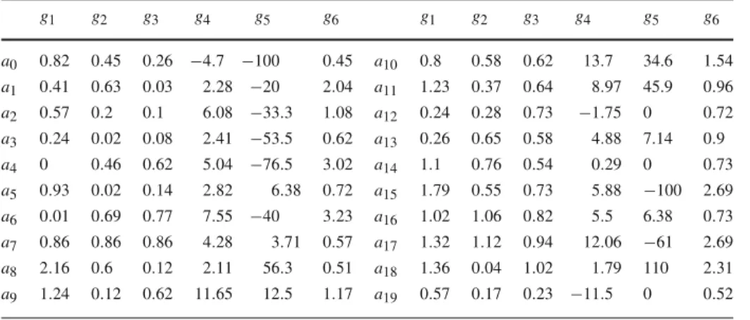
Table 1 Evaluations on six criteria for 20 stocks g1 g2 g3 g4 g5 g6 g1 g2 g3 g4 g5 g6 a0 0.82 0.45 0.26 −4.7 −100 0.45 a10 0.8 0.58 0.62 13.7 34.6 1.54 a1 0.41 0.63 0.03 2.28 −20 2.04 a11 1.23 0.37 0.64 8.97 45.9 0.96 a2 0.57 0.2 0.1 6.08 −33.3 1.08 a12 0.24 0.28 0.73 −1.75 0 0.72 a3 0.24 0.02 0.08 2.41 −53.5 0.62 a13 0.26 0.65 0.58 4.88 7.14 0.9 a4 0 0.46 0.62 5.04 −76.5 3.02 a14 1.1 0.76 0.54 0.29 0 0.73 a5 0.93 0.02 0.14 2.82 6.38 0.72 a15 1.79 0.55 0.73 5.88 −100 2.69 a6 0.01 0.69 0.77 7.55 −40 3.23 a16 1.02 1.06 0.82 5.5 6.38 0.73 a7 0.86 0.86 0.86 4.28 3.71 0.57 a17 1.32 1.12 0.94 12.06 −61 2.69 a8 2.16 0.6 0.12 2.11 56.3 0.51 a18 1.36 0.04 1.02 1.79 110 2.31 a9 1.24 0.12 0.62 11.65 12.5 1.17 a19 0.57 0.17 0.23 −11.5 0 0.52
Table 2 Indifference and preference thresholds
g1 g2 g3 g4 g5 g6
qj 0.05 0.05 0 0.1 8.72 0.05
pj 0.25 0.2 0.2 0.5 10 0.25
strict inequalities in LP1 we usedε=0.00001. Since the DMs of the original studies were not present, and since the results obtained in these studies are not intended to be compared with the ones to be obtained with our procedure, we followed a simple “rule-of-thumb” to provide examples. This rule is to choose for some alternatives the category corresponding to the minimum value in the vector sλi corresponding to them. Of course, in the presence of a real DM, his/her preferences and requirements, based on holistic judgement and experience, should strongly influence the choice of the examples. Hence, these illustrative examples should not be seen as indicating a way to automatically sort the alternatives.
5.1 First example
We will use data form an application for sorting stocks listed in the Athens Stock Exchange [7], namely 20 alternatives from the commercial sector, which were evaluated on 6 criteria (Table1). The criteria names are not relevant here, therefore we will note only that all criteria are to be maximized, except g3(.), where the lower the values, the better. Three categories are to be used: C1(“not attractive”), C2(“uncertain”), and C3(“attractive”, the best category).
We will use the original values [7] for the indifference and preference thresholds (Table2), but we will not use the veto thresholds, i.e., we will ignore discordance. This occurs, in this particular example, because the original values for the veto thresholds led to many veto situations. Since our procedure is based on varying weights and the cutting level to see if it is possible to avoid all the outrankings forbidden by (5), having many veto situations is undesirable to the extent that many of the forbidden outrankings will not hold regardless of the weights and the cutting level values.
The remaining parameters are considered as variables. The cutting levelλcan assume val-ues in[0,1], whereas the weight vectors are constrained to a polytope K defined as suggested in Sect. 4.1. (no criterion is preponderant and no criterion is negligible):
K = {(k1, . . . ,k6):1/12≤kj ≤3/12(j=1, . . . ,6)∧k1+k2+. . .+k6 =1}.
Let us suppose the DM starts by stating one example for each of the three categories:
a3→C1, a14→C2, and a11→C3, i.e., A∗=C1∪C2∪C3, with C1= {a3}, C2= {a14},
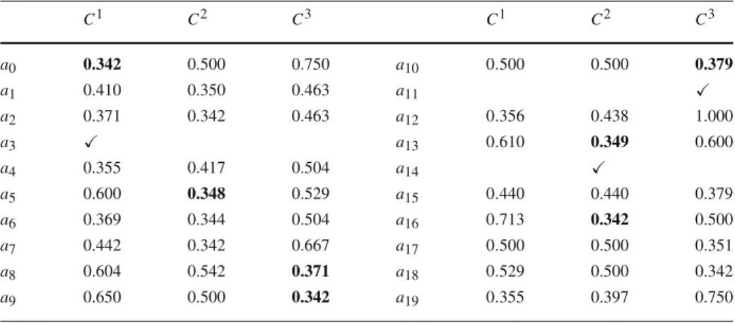
and C3 = {a11}. Table3depicts the optimal valuesλ∗i,hof (LP1) for each potential way of sorting the remaining alternatives in A\A∗.
If as usual in ELECTRE the DM states thatλwill be at least 0.5, then any sorting pos-sibility withλ∗i,h < 0.5 will be feasible (the sorting is possible for anyλ∈ [λ∗i,h,1]). For instance, we may see that alternative a0 can perfectly be sorted into C1 or C2. However,
sorting a0into C3would require acceptingλ≥0.75, which might be considered too high. If
the DM considered thatλ≥0.60 would already be too high, then the alternative a13could be
placed only in C2. Concerning the remaining alternatives, there are typically two categories (sometimes three) where each one could easily be placed. This lack of constraints is natural given the scarce information used up to this moment. In the absence of a DM, we will choose as a set of new examples those that had only one element in siλlower than 0.5: a0 →C1, a5, a13, and a16are sorted into C2, a8, a9, and a10are sorted into C3. The results are now
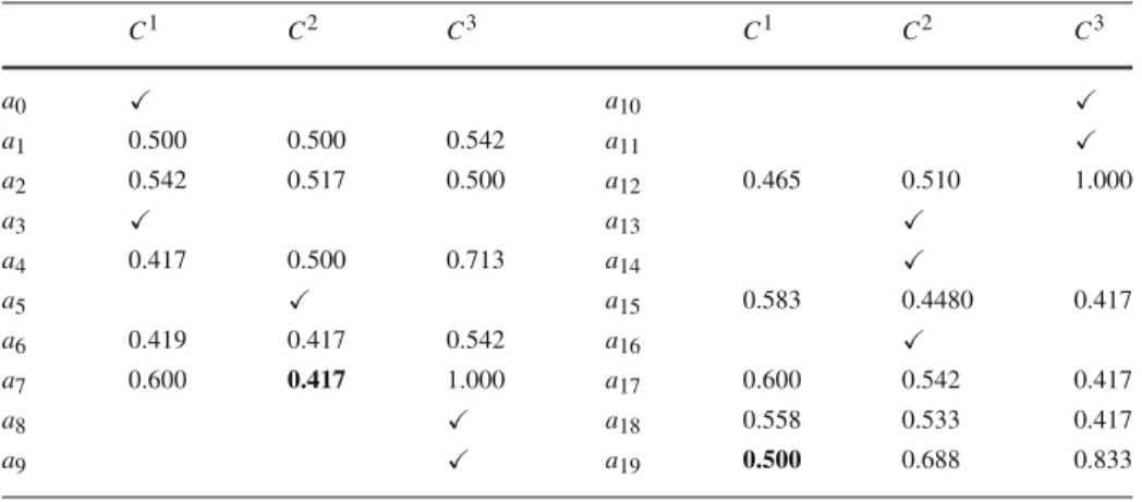
those depicted in Table4, where it can be seen that each value forλ∗i,his not lower than the respective value in Table3. This is natural, since the minimum value of the linear program (LP1) does not decrease as new constraints are added.
Again, we remind that this procedure is not to be followed in such an automatic way. Rather, the holistic evaluations of the DM should play the main role. As a matter of fact, when the most obvious choices are made (e.g., considering at this point adding a7 →C2
and a19→C1, two situations whereλ∗i,his clearly low compared with the other sorting
pos-sibilities for the same alternatives), they are not likely to add much information. Therefore, we will continue now considering a4→C1, a2,a7→C2, and a17→C3, where a2→C2
would not be an obvious choice for sorting a2, but would be the result of a request by the
DM. The corresponding results are provided in Table5.
Table 3 Minimum cutting levelsλ∗i,hfor sorting the alternatives at iteration 1
C1 C2 C3 C1 C2 C3 a0 0.342 0.500 0.750 a10 0.500 0.500 0.379 a1 0.410 0.350 0.463 a11 a2 0.371 0.342 0.463 a12 0.356 0.438 1.000 a3 a13 0.610 0.349 0.600 a4 0.355 0.417 0.504 a14 a5 0.600 0.348 0.529 a15 0.440 0.440 0.379 a6 0.369 0.344 0.504 a16 0.713 0.342 0.500 a7 0.442 0.342 0.667 a17 0.500 0.500 0.351 a8 0.604 0.542 0.371 a18 0.529 0.500 0.342 a9 0.650 0.500 0.342 a19 0.355 0.397 0.750
Table 4 Minimum cutting levelsλ∗i,hfor sorting the alternatives at iteration 2 C1 C2 C3 C1 C2 C3 a0 a10 a1 0.500 0.500 0.542 a11 a2 0.542 0.517 0.500 a12 0.465 0.510 1.000 a3 a13 a4 0.417 0.500 0.713 a14 a5 a15 0.583 0.4480 0.417 a6 0.419 0.417 0.542 a16 a7 0.600 0.417 1.000 a17 0.600 0.542 0.417 a8 a18 0.558 0.533 0.417 a9 a19 0.500 0.688 0.833
Table 5 Minimum cutting levelsλ∗i,hfor sorting the alternatives at iteration 3
C1 C2 C3 C1 C2 C3 a0 a10 a1 0.613 0.500 0.546 a11 a2 a12 0.465 0.522 1.000 a3 a13 a4 a14 a5 a15 0.583 0.474 0.486 a6 0.542 0.417 0.542 a16 a7 a17 a8 a18 0.558 0.575 0.500 a9 a19 0.515 0.688 0.833
Table 6 Minimum cutting levelsλ∗i,hfor sorting the alternatives at iteration 4
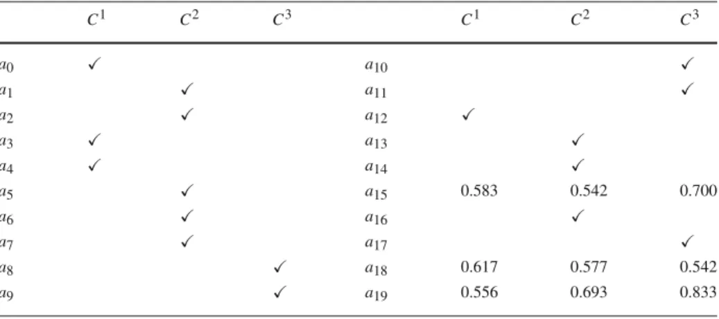
C1 C2 C3 C1 C2 C3 a0 a10 a1 a11 a2 a12 a3 a13 a4 a14 a5 a15 0.750 0.750 0.700 a6 a16 a7 a17 a8 a18 a9 a19 0.556 0.693 0.833
Table 7 Minimum cutting levelsλ∗i,hfor sorting the alternatives after removing example a18→C3 C1 C2 C3 C1 C2 C3 a0 a10 a1 a11 a2 a12 a3 a13 a4 a14 a5 a15 0.583 0.542 0.700 a6 a16 a7 a17 a8 a18 0.617 0.577 0.542 a9 a19 0.556 0.693 0.833
Table 8 Performances of the alternatives to be sorted (second example)
g1 g2 g3 g4 g5 g6 g7 g1 g2 g3 g4 g5 g6 g7 a0 35.8 67.0 19.7 0.0 0.0 5.0 4.0 a20 15.5 8.5 56.2 5.5 1.8 4.0 2.0 a1 16.4 14.5 59.8 7.5 5.2 5.0 3.0 a21 13.2 9.1 74.1 6.4 5.0 2.0 2.0 a2 35.8 24.0 64.9 2.1 4.5 5.0 4.0 a22 9.1 4.1 44.8 3.3 10.4 3.0 4.0 a3 20.6 61.7 75.7 3.6 8.0 5.0 3.0 a23 12.9 1.9 65.0 14.0 7.5 4.0 3.0 a4 11.5 17.1 57.1 4.2 3.7 5.0 2.0 a24 5.9 −27.7 77.4 16.6 12.7 3.0 2.0 a5 22.4 25.1 49.8 5.0 7.9 5.0 3.0 a25 16.9 12.4 60.1 5.6 5.6 3.0 2.0 a6 23.9 34.5 48.9 2.5 8.0 5.0 3.0 a26 16.7 13.1 73.5 11.9 4.1 2.0 2.0 a7 29.9 44.0 57.8 1.7 2.5 5.0 4.0 a27 14.6 9.7 59.5 6.7 5.6 2.0 2.0 a8 8.7 5.4 27.4 4.5 4.5 5.0 2.0 a28 5.1 4.9 28.9 2.5 46.0 2.0 2.0 a9 25.7 29.7 46.8 4.6 3.7 4.0 2.0 a29 24.4 22.3 32.8 3.3 5.0 3.0 4.0 a10 21.2 24.6 64.8 3.6 8.0 4.0 2.0 a30 29.5 8.6 41.8 5.2 6.4 2.0 3.0 a11 18.3 31.6 69.3 2.8 3.0 4.0 3.0 a31 7.3 −64.5 67.5 30.1 8.7 3.0 3.0 a12 20.7 19.3 19.7 2.2 4.0 4.0 2.0 a32 23.7 31.9 63.6 12.1 10.2 3.0 2.0 a13 9.9 3.5 53.1 8.5 5.3 4.0 2.0 a33 18.9 13.5 74.5 12.0 8.4 3.0 3.0 a14 10.4 9.3 80.9 1.4 4.1 4.0 2.0 a34 13.9 3.3 78.7 14.7 10.1 2.0 2.0 a15 17.7 19.8 52.8 7.9 6.1 4.0 4.0 a35 −13.3 −31.1 63.0 21.2 29.1 2.0 1.0 a16 14.8 15.9 27.9 5.4 1.8 4.0 2.0 a36 6.2 −3.2 46.1 4.8 10.5 2.0 1.0 a17 16.0 14.7 53.5 6.8 3.8 4.0 4.0 a37 4.8 −3.3 71.1 8.6 11.6 2.0 2.0 a18 11.7 10.0 42.1 12.2 4.3 5.0 2.0 a38 0.1 −9.6 42.5 12.9 12.4 1.0 1.0 a19 11.0 4.2 60.8 6.2 4.8 4.0 2.0 a39 13.6 9.1 76.0 17.1 10.3 1.0 1.0
Sorting many alternatives at each iteration increases the risk of reaching an inconsistency situation. For instance, let us suppose the DM decided to sort all the remaining alternatives except a15 and a19to the categories where the valueλ∗i,h was minimum. This would lead
to the results in Table6, where the DM must accept a cutting level of at least 0.7 to sort
a15. If we suppose this was considered too high by the DM, then some examples would have to be withdrawn. To inform this decision, one may check which constraints of (LP1)
are binding at the optimal solutions concerning a15, which would show that the example
concerning a18is responsible for the high values inλ∗15,1andλ∗15,2. Withdrawing only the
example a18(removing the alternative from C3) leads to Table7. At this point the DM could
decide a15 →C2, which would not change s∗19. Then, a19→C1would be a natural
con-tinuation for this process, yielding s18∗ =(0.617,0.577,0.750). Finally, a18→C2could be
the natural ending for this process. 5.2 Second example
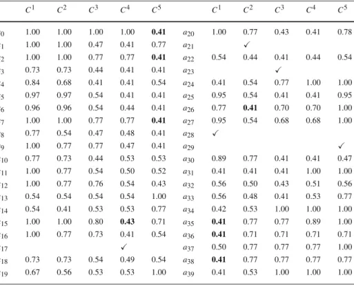
We will now present a second example with more alternatives to sort and more categories. We will use data from [4], referring to the evaluation of 40 companies to be sorted into 5
cate-Table 9 Thresholds associated with the criteria
g1 g2 g3 g4 g5 g6 g7
qj 1 4 1 1 0 0 0
pj 2 6 3 2 3 0 0
uj 35 90 45 20 35 3.5 3.5
vj 45 120 55 30 45 6.5 6.5
Table 10 Minimum cutting levelsλ∗i,hat iteration 1 (2nd example)
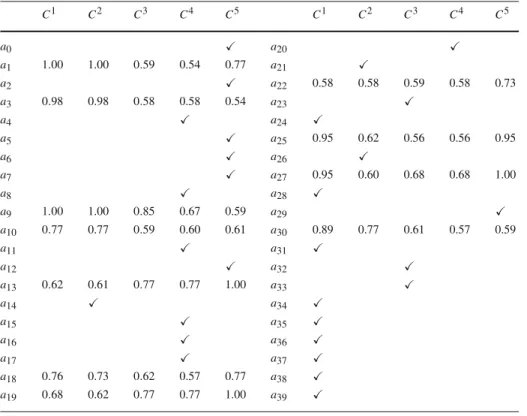
C1 C2 C3 C4 C5 C1 C2 C3 C4 C5 a0 1.00 1.00 1.00 1.00 0.41 a20 1.00 0.77 0.43 0.41 0.78 a1 1.00 1.00 0.47 0.41 0.77 a21 a2 1.00 1.00 0.77 0.77 0.41 a22 0.54 0.44 0.41 0.44 0.54 a3 0.73 0.73 0.44 0.41 0.41 a23 a4 0.84 0.68 0.41 0.41 0.54 a24 0.41 0.54 0.77 1.00 1.00 a5 0.97 0.97 0.54 0.41 0.41 a25 0.95 0.54 0.41 0.41 0.95 a6 0.96 0.96 0.54 0.44 0.41 a26 0.77 0.41 0.70 0.70 1.00 a7 1.00 1.00 0.77 0.77 0.41 a27 0.95 0.54 0.68 0.68 1.00 a8 0.77 0.54 0.47 0.48 0.41 a28 a9 1.00 0.77 0.77 0.47 0.41 a29 a10 0.77 0.73 0.44 0.53 0.53 a30 0.89 0.77 0.41 0.41 0.47 a11 1.00 0.77 0.54 0.50 0.52 a31 0.41 0.41 0.41 1.00 1.00 a12 1.00 0.77 0.76 0.54 0.43 a32 0.56 0.50 0.43 0.51 0.56 a13 0.54 0.54 0.54 0.54 1.00 a33 0.56 0.48 0.41 0.53 0.77 a14 0.54 0.41 0.53 0.53 0.77 a34 0.42 0.53 1.00 1.00 1.00 a15 1.00 1.00 0.80 0.43 0.71 a35 0.41 0.77 0.77 0.89 1.00 a16 1.00 0.77 0.73 0.41 0.54 a36 0.41 0.71 0.71 0.71 0.71 a17 a37 0.50 0.77 0.77 0.77 1.00 a18 0.73 0.73 0.54 0.49 0.54 a38 0.41 0.77 0.77 0.77 0.77 a19 0.67 0.56 0.53 0.53 1.00 a39 0.41 0.53 1.00 1.00 1.00
gories (in the original application there were only 3 categories) representing their risk, based on their performances on 7 criteria. Criteria g1, g2, g6, and g7are to be maximized, whereas g3, g4, and g5are to be minimized. Table8depicts the performances of the alternatives on
these criteria.
We will consider as fixed the indifference, preference, discordance, and veto thresholds associated with each criterion, indicated in Table9. We now enable discordance to occur, although we have chosen values for uj andvj that do not allow veto situations to occur frequently when comparing the alternatives.
The remaining parameters are again considered as variables. The cutting levelλ can assume values in[0,1], whereas the weight vectors are constrained to a polytope K defined as suggested in Sect. 4.1:
K = {(k1, . . . ,k7):2/35≤kj ≤8/35(j=1, . . . ,7)∧k1+k2+. . .+k7 =1}. Let us suppose the DM starts by stating one example for each of the five categories:
a28→C1, a21→C2, a23→C3, a17→C4, and a29→C5. Table10depicts the optimal
valuesλ∗i,hof (LP1) for each potential way of sorting the remaining alternatives in A\A∗. Despite the scarce information used, there are some possible assignments that are very natural to accept, such as sorting a0into C5. If we hypothesize that the DM wants to consider a
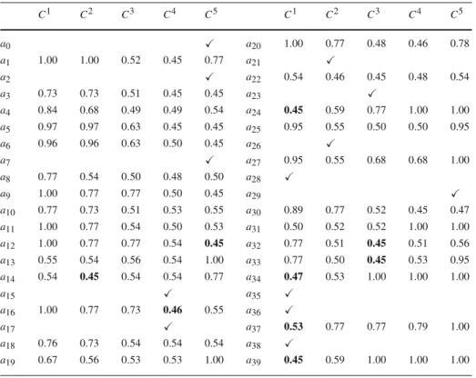
cutting level lower than 0.7, then the following examples could be also added: a35,a36,a38→ C1, a
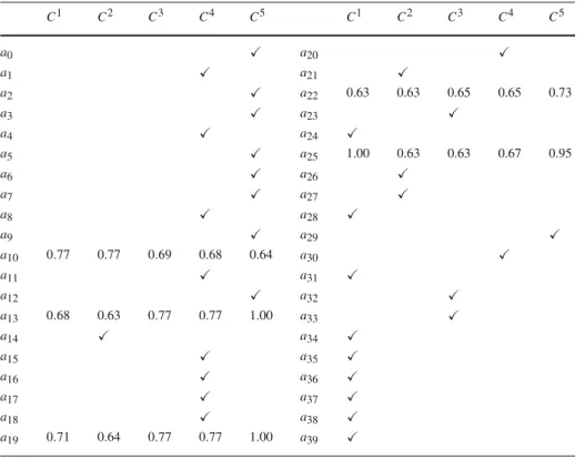
26→C2, a15→C4, a0,a2,a7→C5. Adding these examples would lead to the results
Table 11 Minimum cutting levelsλ∗i,hat iteration 2 (2nd example)
C1 C2 C3 C4 C5 C1 C2 C3 C4 C5 a0 a20 1.00 0.77 0.48 0.46 0.78 a1 1.00 1.00 0.52 0.45 0.77 a21 a2 a22 0.54 0.46 0.45 0.48 0.54 a3 0.73 0.73 0.51 0.45 0.45 a23 a4 0.84 0.68 0.49 0.49 0.54 a24 0.45 0.59 0.77 1.00 1.00 a5 0.97 0.97 0.63 0.45 0.45 a25 0.95 0.55 0.50 0.50 0.95 a6 0.96 0.96 0.63 0.50 0.45 a26 a7 a27 0.95 0.55 0.68 0.68 1.00 a8 0.77 0.54 0.50 0.48 0.50 a28 a9 1.00 0.77 0.77 0.50 0.45 a29 a10 0.77 0.73 0.51 0.53 0.55 a30 0.89 0.77 0.52 0.45 0.47 a11 1.00 0.77 0.54 0.50 0.53 a31 0.50 0.52 0.52 1.00 1.00 a12 1.00 0.77 0.77 0.54 0.45 a32 0.77 0.51 0.45 0.51 0.56 a13 0.55 0.54 0.56 0.54 1.00 a33 0.77 0.50 0.45 0.53 0.95 a14 0.54 0.45 0.54 0.54 0.77 a34 0.47 0.53 1.00 1.00 1.00 a15 a35 a16 1.00 0.77 0.73 0.46 0.55 a36 a17 a37 0.53 0.77 0.77 0.79 1.00 a18 0.76 0.73 0.54 0.54 0.54 a38 a19 0.67 0.56 0.53 0.53 1.00 a39 0.45 0.59 1.00 1.00 1.00
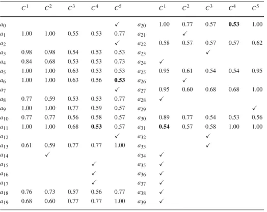
Table 12 Minimum cutting levelsλ∗i,hat iteration 3 (2nd example) C1 C2 C3 C4 C5 C1 C2 C3 C4 C5 a0 a20 1.00 0.77 0.57 0.53 1.00 a1 1.00 1.00 0.55 0.53 0.77 a21 a2 a22 0.58 0.57 0.57 0.57 0.62 a3 0.98 0.98 0.54 0.53 0.53 a23 a4 0.84 0.68 0.53 0.53 0.73 a24 a5 1.00 1.00 0.63 0.53 0.53 a25 0.95 0.61 0.54 0.54 0.95 a6 1.00 1.00 0.63 0.56 0.53 a26 a7 a27 0.95 0.60 0.68 0.68 1.00 a8 0.77 0.59 0.53 0.53 0.77 a28 a9 1.00 1.00 0.77 0.59 0.57 a29 a10 0.77 0.77 0.56 0.58 0.57 a30 0.89 0.77 0.54 0.53 0.56 a11 1.00 1.00 0.68 0.53 0.57 a31 0.54 0.57 0.58 1.00 1.00 a12 a32 a13 0.61 0.59 0.77 0.77 1.00 a33 a14 a34 a15 a35 a16 a36 a17 a37 a18 0.76 0.73 0.57 0.56 0.77 a38 a19 0.68 0.60 0.77 0.77 1.00 a39
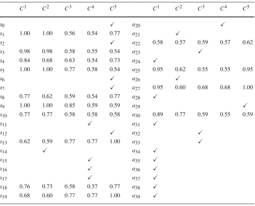
in Table11. Tables12–16present a possible sequence based on a systematical choice of the lowerλ∗i,hvalues.
After the last iteration, only two alternatives remain to be sorted: a22 and a25. There
remains some freedom concerning how to sort them. For instance, sorting a22into C1, C2, C3, or C4(C5would require a higher cutting level) does not change the values of sλ
25,
mean-ing it allows sortmean-ing a25into one of the three categories in the interval[C2,C4]. Likewise,
sorting a25into one of the three categories in the interval[C2,C4]does not constrain the
sorting possibilities for a22. Therefore, the procedure would not be of further help to the DM
concerning how to sort these two alternatives.
6 Conclusion
This work presented a PASA based on the ELECTRE methodology. Its purpose is to support a DM who does not wish to provide a formal and explicit definition for the categories in an ordinal sorting problem. Rather, the categories can be seen as subjective qualitative evalua-tion levels vaguely established in the DM’s mind. The PASA supports the DM by enforcing the principle (5): “if an alternative outranks (is as good as) a second one, then it must be placed on the same category or in a better category”.
We have shown that if the outranking relation is completely defined (all the parameter values are fixed), then it is possible to constrain the range of categories where an alternative
Table 13 Minimum cutting levelsλ∗i,hat iteration 4 (2nd example) C1 C2 C3 C4 C5 C1 C2 C3 C4 C5 a0 a20 a1 1.00 1.00 0.56 0.54 0.77 a21 a2 a22 0.58 0.57 0.59 0.57 0.62 a3 0.98 0.98 0.58 0.55 0.54 a23 a4 0.84 0.68 0.63 0.54 0.73 a24 a5 1.00 1.00 0.77 0.58 0.54 a25 0.95 0.62 0.55 0.55 0.95 a6 a26 a7 a27 0.95 0.60 0.68 0.68 1.00 a8 0.77 0.62 0.59 0.54 0.77 a28 a9 1.00 1.00 0.85 0.59 0.59 a29 a10 0.77 0.77 0.58 0.58 0.58 a30 0.89 0.77 0.59 0.55 0.59 a11 a31 a12 a32 a13 0.62 0.59 0.77 0.77 1.00 a33 a14 a34 a15 a35 a16 a36 a17 a37 a18 0.76 0.73 0.58 0.57 0.77 a38 a19 0.68 0.60 0.77 0.77 1.00 a39
may be sorted given sorting examples previously expressed. We have also shown how the same idea may be used in an aggregation/disaggregation approach, considering the weights and the cutting level are not fixed a priori, but constrained by the examples provided. In this context, we established a “convex-shape property” that shows that there are no “holes” in the range of possible categories for an alternative: if it can be placed in Cx and Cy, then it can be placed in any category in[Cx,Cy].
Finally, we have proposed, and we have illustrated with some examples, a process based on the computation of the minimum cutting levelλ∗i,hneeded to allow an alternative aito be sorted into a category Ch.
The spirit of the approach proposed in this paper is that of aiding a DM to perform sorting decisions in a consistent manner, rather than deriving a model to substitute the DM. Each sorting decision will constrain the subsequent ones if consistency with principle (5) is to be maintained. Therefore, the DM is aided when the procedure shows what is the minimum and maximum category where an alternative might be sorted. Sometimes, the minimum and maximum will coincide. Some other times, it is up to the DM to make the decision. In this sense, the procedure both assists the DM and is assisted by the DM. The DM assists the pro-cedure by choosing one among a range of potential categories for an alternative. On the other hand, the DM will be assisted subsequently as the newly sorted alternative may contribute to narrow the interval of possible categories for future alternatives.
Comparing this approach with ELECTRE TRI and its aggregation/disaggregation exten-sions [3], the most salient feature of the approach proposed in this paper is that the explicit
Table 14 Minimum cutting levelsλ∗i,hat iteration 5 (2nd example) C1 C2 C3 C4 C5 C1 C2 C3 C4 C5 a0 a20 a1 1.00 1.00 0.59 0.54 0.77 a21 a2 a22 0.58 0.58 0.59 0.58 0.73 a3 0.98 0.98 0.58 0.58 0.54 a23 a4 a24 a5 a25 0.95 0.62 0.56 0.56 0.95 a6 a26 a7 a27 0.95 0.60 0.68 0.68 1.00 a8 a28 a9 1.00 1.00 0.85 0.67 0.59 a29 a10 0.77 0.77 0.59 0.60 0.61 a30 0.89 0.77 0.61 0.57 0.59 a11 a31 a12 a32 a13 0.62 0.61 0.77 0.77 1.00 a33 a14 a34 a15 a35 a16 a36 a17 a37 a18 0.76 0.73 0.62 0.57 0.77 a38 a19 0.68 0.62 0.77 0.77 1.00 a39
definition of category limits (profiles) is avoided. However, contrarily to other approaches that define categories on the basis of exemplary alternatives (e.g., [1]), we use the outranking relation in an asymmetrical way, rather than being interested in an indifference relation.
Avoiding the definition of category limits may be considered as an advantage of this procedure, as inferring the category limits is not an easy task without imposing a few sim-plifications [16]. In any case, we are indirectly defining multiple limits. In ELECTRE TRI (pessimistic variant), an alternative is sorted into a category if it outranks its lower limit and does not outrank its upper limit, with lower and upper limits defined a priori. In this paper, an alternative is sorted into a category if it is not outranked by a lower limit and does not outrank an upper limit, with lower and upper limits being any alternative already sorted by the DM in worse or better categories, respectively.
Both the procedure proposed here and ELECTRE TRI have the common characteristic of not sorting an alternative into a precise category if that alternative shows to be atypical. In ELECTRE TRI this is reflected in different results between the pessimistic and optimistic variants, which appear when the alternative to be sorted is incomparable to one or more limits. In this paper, the procedure in Sect.3may also result in Cmi n(ai) =Cmax(ai), if the alternative is incomparable to all the examples placed in a given category. However, if the DM then decides to consider that alternative as an example for one of the categories in
[Cmi n(ai),Cmax(ai)], then subsequent similar alternatives will use that example to justify a more precise classification. As the number of sorted alternatives increases, the chance of
Table 15 Minimum cutting levelsλ∗i,hat iteration 6 (2nd example) C1 C2 C3 C4 C5 C1 C2 C3 C4 C5 a0 a20 a1 a21 a2 a22 0.63 0.63 0.65 0.65 0.73 a3 a23 a4 a24 a5 a25 1.00 0.63 0.63 0.67 0.95 a6 a26 a7 a27 a8 a28 a9 a29 a10 0.77 0.77 0.69 0.68 0.64 a30 a11 a31 a12 a32 a13 0.68 0.63 0.77 0.77 1.00 a33 a14 a34 a15 a35 a16 a36 a17 a37 a18 a38 a19 0.71 0.64 0.77 0.77 1.00 a39
finding an atypical alternative decreases. The downside is that as the number of examples increases, so does the chance of being inconsistent.
Since the examples can be fictitious vectors of performances invented by the DM (as usually are the limits in ELECTRE TRI), our paper can be interpreted as proposing an exten-sion of ELECTRE TRI to allow multiple limits (probably incomparable ones) separating the categories. The main difference would then be the fact that the condition of outranking the lower limit is replaced by the condition of not being outranked by a lower limit. This use of this approach would place each alternative in the lowest category allowed by the principle (5) (pessimistic variant), or in the highest category possible (optimistic variant). If the principle (5) is to be strictly followed, as sustained in this paper, then it must apply to all the alternatives that are sorted by the DM. Nevertheless, the DM can select not to consider all alternatives as examples, i.e., not to sort all alternatives to precise categories. This means that the set A∗ would strictly follow the principle (5), serving as prototypes to constrain the sorting of the remaining alternatives ai ∈ A\A∗to an interval[Cmi n(ai),Cmax(ai)](Cmi n(ai)being the result of a pessimistic procedure, and Cmax(ai)being the result of an optimistic procedure). Comparing the aggregation/disaggregation approach proposed here with the one proposed for ELECTRE TRI, another difference is to have only negative outranking (i.e., non-outran-king) constraints of the typeλ−S(ap,ai)≥ε, whereas for ELECTRE TRI we have positive (λ−S(ap,ai)≤0) as well as negative outranking constraints. Therefore, in this paper we do not infer a value for the cutting levelλ(we know thatλ=1 would trivially solve almost all of the constraints), but we infer a minimum value for this parameter. This forces the DM
Table 16 Minimum cutting levelsλ∗i,hat iteration 7 (2nd example) C1 C2 C3 C4 C5 C1 C2 C3 C4 C5 a0 a20 a1 a21 a2 a22 0.66 0.65 0.67 0.67 0.73 a3 a23 a4 a24 a5 a25 1.00 0.65 0.65 0.67 0.95 a6 a26 a7 a27 a8 a28 a9 a29 a10 a30 a11 a31 a12 a32 a13 a33 a14 a34 a15 a35 a16 a36 a17 a37 a18 a38 a19 a39
to deal explicitly with the meaning of the cutting level when deciding in which categories may each alternative be sorted into, which may be seen as the price to pay in this approach to avoid the definition of category limits.
Finding appropriate ways of incorporating positive outranking constraints in this approach is an interesting issue to research in the future. Future research is also needed to evaluate the implications of the number and choice of examples in the results of the procedure. This involves not only to continue experimenting with examples such as the ones presented here, but also possibly performing simulation studies.
Acknowledgement This work has been supported by FCT/FEDER grant POCI 2010/EGE/58371/2004. References
1. Belacel, N.: Multicriteria assignment method PROAFTN: methodology and medical application. Euro-pean J. Oper. Res. 125(1), 175–183 (2000)
2. Bilgin, S., Köksalan, M., Mousseau, V., Özpeynirci, O.: A new outranking-based approach for assigning alternatives to ordered classes. Communication to the 18th International Conference on Multiple Criteria Decision Making. pp. 19–23. Chania, Greece (2006)
3. Dias, L.C., Mousseau, V., Figueira, J., Clímaco, J.N.: An aggregation/disaggregation approach to obtain robust conclusions with ELECTRE TRI. European J. Oper. Res. 138(2), 332–348 (2002)
4. Dimitras, A., Zopounidis, C., Hurson, C.: A multicriteria decision aid method for the assessment of business failure risk. Found. Comput. Decision Sci. 20(2), 99–112 (1995)