Bayesian Biclustering on Discrete Data: Variable Selection Methods

(1)

Bayesian Biclustering on Discrete Data: Variable Selection

Methods

(Article begins on next page)

The Harvard community has made this article openly available.

Please share

how this access benefits you. Your story matters.

Citation

Guo, Lei. 2013. Bayesian Biclustering on Discrete Data: Variable

_{Selection Methods. Doctoral dissertation, Harvard University.}

Accessed

April 17, 2018 4:22:44 PM EDT

Citable Link

http://nrs.harvard.edu/urn-3:HUL.InstRepos:11181216

Terms of Use

This article was downloaded from Harvard University's DASH

_{repository, and is made available under the terms and conditions}

applicable to Other Posted Material, as set forth at

http://nrs.harvard.edu/urn-3:HUL.InstRepos:dash.current.terms-of-use#LAA

(2)

Bayesian Biclustering on Discrete Data: Variable

Selection Methods

A dissertation presented by Lei Guo to

The Department of Statistics in partial fulfillment of the requirements

for the degree of Doctor of Philosophy in the subject of Statistics Harvard University Cambridge, Massachusetts September 2013

(3)

c 2013 - Lei Guo

(4)

Dissertation Advisor: Jun S. Liu Lei Guo

Bayesian Biclustering on Discrete Data: Variable Selection

Methods

Abstract

Biclustering is a technique for clustering rows and columns of a data matrix simul-taneously. Over the past few years, we have seen its applications in biology-related fields, as well as in many data mining projects. As opposed to classical clustering methods, biclustering groups objects that are similar only on a subset of variables. Many biclustering algorithms on continuous data have emerged over the last decade. In this dissertation, we will focus on two Bayesian biclustering algorithms we devel-oped for discrete data, more specifically categorical data and ordinal data.

The international HapMap project has made available the single-nucleotide poly-morphism (SNP) data of thousands of individuals across the world. We analyzed the SNPs data with our biclustering algorithm for categorical data and described the similarities between human populations. In contrast to existing methods, our method can locate the SNPs that are specific to subpopulation groups. This can provide in-sight to the genome-wide association study (GWAS) by eliminating SNPs that are common to di↵erent ethic groups. We also identified a number of SNPs that are linked to disease, and this thesis describes their behavior in di↵erent subpopulations. The biclustering process can be used as a variable selection step prior to existing population inference procedures.

(5)

The successful completion of my PhD has been a memorable moment in my life with the best years of my life spent at the Harvard University; Department of Statis-tics, where I was able to work with some of the most brilliant minds in the world. During this journey, I am grateful to many individuals who have contributed to my educational, personal and professional development and who have truly helped me to present meaningful knowledge to the world through years of research.

I am forever grateful to my advisor, Prof. Jun S. Liu as this dissertation would not have been possible without his constant guidance, encouragement, unyielding support and patience. I also sincerely appreciate the help from the rest of my thesis committee, which includes Prof. Tirthankar Dasgupta and Prof. David P. Harrington.

In addition, I would like to thank other faculty and sta↵ members of the De-partment of Statistics and the Harvard community, which include Edoardo Airoldi, Joseph K. Blitzstein, Betsey Cogswell, Steven Finch, S.C. Samuel Kou, James Mate-jek, Xiao-Li Meng, Luke W. Miratrix, Carl N. Morris, Alice Moses, Dale Rinkel, Donald B. Rubin, Maureen Stanton, and Darryl E. Zeigler.

For my entire PhD life I’ve been so fortunate to work with my amazing labmates, and I would like to thank: Ke Deng, Jiong Du, Daniel Fernandez, Simeng Han, Bo Jiang, Yang Li, Xuxin Liu, Yang Liu, Ping Ma, Di Wu, Jiexing Wu, Chao Ye for their enduring encouragement, camaraderie and the wonderful memories that they have provided for a lifetime.

Throughout this time, my parents have fully supported me and have given me endless help and encouragement. I am extremely blessed to have them in my life and proud to be their son.

(8)

Acknowledgments

This long journey would not have been the same without the support of my friends and special thanks go to: Rex G. Baker IV, Nickolas P. Chelyapov, Amanda Cheng, Chao Du, Linglan Gong, Jian Guo, Oliver Hayen, Konstantina Karterouli, Xiaoyan Peng, Melissa Rick, Lei Shen, Nan Shen, Yujun Wu, Ying Yan and Rie Yano.

(9)

(10)

Chapter 1 Introduction

Clustering is the art of organizing similar objects into groups according to their variables so that objects are more similar to each other within each groups. It is a common technique in statistical data analysis, and has applications in many fields, e.g., biological sequence analysis, population structure inference, medical imaging, market research, social networking analysis, recommender systems, search engine op-timization, etc.

Central to the problem of clustering is how one defines a ”cluster.” The notion of a cluster can be defined in many ways, resulting in many di↵erent clustering algorithms (Estivill-Castro (2002)). Typical cluster models include connectivity models, which choose a measure of distance and then perform clustering based on distance con-nectivity; centroid models, which characterize clusters using a single centroid vector; distribution models, which employ statistical models to describe the clusters; density models, which define clusters as connected dense regions in the data space; subspace models, which select a subset of attributes and define clusters based on this subset of

(11)

Chapter 1: Introduction

space; etc. Subspace models are also called biclustering, or two-way clustering, which is the model this dissertation will explore in more detail in the following chapters.

Clustering algorithms produce di↵erent results based on their particular defini-tions of ”cluster.” Connectivity-based hierarchical clustering treats clusters as closely connective objects, and describes a cluster by the maximum distance to connect all parts of such cluster. There are also multiple choices for distance measure, e.g., sin-gle linkage, complete linkage, average linkage, ward, median, etc. More clusters will form as distance increases, and this can be represented with a dendrogram, with the x-axis as the objects and the y-axis as the distance for the clusters to merge. There is no single partitioning of the data set but a hierarchy of clusters at di↵erent levels. K-means is another popular clustering algorithm based on centroid models. Given K (the number of clusters) the algorithm iteratively assigns each object into its nearest cluster and calculates the cluster’s centroid. This is a NP-hard optimization problem and can usually be approximated. The clustering model most used by statisticians is distribution model-based clustering, or model-based clustering. The major bene-fit of model-based clustering is that the clusters are clearly defined as /textitobjects that share the same distribution. The interpretation of the clustering results is also straightforward, with each fitted parameter having its context based meanings. How-ever, a known problem with model based clustering is overfitting. When we add more parameters into the model, we can always explain the data better, but the complex-ity of the model grows. Model complexcomplex-ity penalties are necessary for choosing the appropriate model.

(12)

over a subset of variables. The concept was first introduced by Hartigan (1972), and the termbiclustering was coined by Mirkin (1996). However, for almost 30 years, the technique has seen no application in real data. In the year 2000, as more and more gene expression data was becoming available, Cheng and Church reintroduced the same concept and applied it to the gene expression data of yeast (Cheng and Church (2000)).

To further illustrate the concept, let us consider a rectangular matrix M, with

I rows and J columns. Rows represent objects and columns represent features or variables. Biclustering algorithms seek to find a sub-matrix: a subset of rows that share similar patterns across a subset of columns. A simple example is consumers’ purchase behavior with respect to clothing. Variables for clothes include color, style, material, texture, size, etc. Some people may only consider style, color, and texture when making a purchase, while other people may care about style and material. Based on the preferences of people, we can divide them into two separate groups, one using style, color and texture variables, the other one using style and material. Those form two biclusters and we used only a subset of the physical properties of clothes for each group. Another example for illustrating the concept of biclustering is the subject matter of documents. After removing commonly used words like a, the,

do, etc., we will have a data matrix. Each row of the matrix represents a document and each column represents the counts of the occurrences of words that appeared in the document. We can thus find a subset of words and use those words to group similar documents together. Each of those groups are assumed to include documents with the same subject matter. For those problems, the data matrix contains many

(13)

variables but the groups are defined only using a subset of the variables. Traditional partitioning methods such ask-means will often produce undesirable results and are not ideal algorithms for classification.

Just as with traditional clustering, di↵erent definitions of biclusters inform dif-ferent biclustering algorithms (Madeira and Oliveira (2004)). There are four major types of biclusters: (a) Biclusters with constant values; (b) Biclusters with constant values on rows (or columns); (c) Biclusters with coherent values (additive or multi-plicative); and(d)Biclusters with coherent evolutions. Many biclustering algorithms have been developed since the application of biclustering to gene expression data, and we will review some notable algorithms in the next chapter.

This dissertation will focus on introducing two new biclustering algorithms, and one related application, to Human SNPs data from the HapMap project. Chapter 2 will give an overview of popular biclustering algorithms and their applications in di↵erent fields. Chapter 3 will introduce the basics of categorical data, drawing exam-ples from di↵erent subjects, and will explain the theoretical background for Bayesian biclustering on categorical data. Chapter 4 will illustrate scenarios relating to the usage of ordinal data, and will also detail the Bayesian framework for biclustering on ordinal data using a Normal Random Cuto↵ approximation model. We also fur-ther extend the biclustering model with the capacity to handle more levels of ordinal data by introducing a Uniform Binomial mixture model. Chapter 5 will focus on the application of the categorical biclustering model to human single-nucleotide polymor-phism (SNP) data from HapMap Phase III, as well as to disease linked SNPs analysis. Therein, we also present significant findings and result analysis.

(14)

Chapter 2 An overview of Biclustering

Methods

2.1 Notation

We will now introduce a few notations to formally definebicluster. These notations will be used throughout the rest of the Chapter.

Suppose we have a data matrix A, with rows as object set X and columns as variable set Y and the entry aij. The purpose of biclustering methods is to find a

sub-matrix of Awith row set I⇢X and column set J⇢Y, such that the I objects are as similar as possible on column set J. This sub-matrixA_{I,J} is called abicluster, as seen in Figure 2.1. We use a.j to denote the mean of thejth column in the bicluster,

ai. as the mean of the ith row in the bicluster, and a.. as the overall mean of all

(15)

Chapter 2: An overview of Biclustering Methods

Figure 2.1: Illustration of a Bicluster. For a single bicluster, after re-arranging rows and columns, we can change it from the configuration on the right panel to the one on the left.

2.2 Types of Biclusters

By the nature of the data, there are two types of biclusters: (a) Biclusters with quantitative values and (b) Biclusters with qualitative values. According to the con-figuations of the biclusters they detect, Madeira and Oliveira (2004) furtherclustered existing biclustering algorithms into four major classes:

(16)

1. Biclusters with constant values.

constant values on rows and columns

aij =µ

2. Biclusters with constant values on columns or rows.

constant values on rows aij =µ+↵i constant values on columns aij =µ+ j

3. Biclusters with coherent values.

additive aij =µ+↵i+ j multiplicative aij =µ·↵i· j

4. Biclusters with coherent evolutions.

Figure 2.2: Illustration of the four major types of biclusters that existing algorithms seek to recover.

(17)

values while di↵erent rows have di↵erent values. In Figure 2.2c, every column has identical values while di↵erent columns have di↵erent values. Figure 2.2b and Figure 2.2c are equivalent if we transpose the data matrix. In Figure 2.2d, every cell is a summation of row e↵ect and column e↵ect, each row has a di↵erent row e↵ect, and similarly for di↵erent columns. In Figure 2.2e, every cell is a multiplication of row e↵ect and column e↵ect, each row has a di↵erent row e↵ect, and similarly for di↵erent columns. Figure 2.2d and Figure 2.2e are essentially the same if we take the logarithm of the data matrix. The first three types of biclustering algorithms deal with the numeric values of the data matrix directly. They aim to find subsets of rows that are similar over corresponding subsets of columns. Because these three types of biclustering use the numeric values of a data matrix directly, many related biclustering algorithms have been developed, which we will illustrate in the following sections.

The fourth type of biclustering algorithm deals with coherent evolutions, regard-less of the real numeric values in the data matrix. The biclustering is performed on an abstract layer of the data. This abstract layer views data as symbols. There are two types of symbols: non-ordered symbols, that is, nominal (categorical); and order-preserving symbols, that is, ordinal. Few algorithms have been developed for coherent evolution data and most of them are simply ad-hoc. This dissertation presents a gen-eral framework for the biclustering of these two types of data, and will present the details thereof in Chapters 3 and 4. Our biclustering algorithm for categorical and ordinal data can handle both numeric matrices and matrices with coherent evolution data. The continuous case for coherent value (additive and multiplicative)

(18)

bicluster-Chapter 2: An overview of Biclustering Methods

ing has been covered by Gu and Liu (2008).

2.3 Patterns of Biclusters

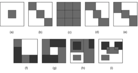
Figure 2.3: Di↵erent structures of biclusters, from Madeira and Oliveira (2004) There are generally more than one bicluster in a data matrix. Let’s assume there areKbiclusters in a data matrix. In the ideal case, after reordering rows and columns of the data matrix, the biclusters may appear as rectangular blocks. Within each of those blocks, the objects are more similar to each other in terms of their values on the chosen subset of columns.

For most algorithms, we assume a neutral background where little information can be captured for the elements outside the bicluster blocks. However, in our model, we do not assume the existence of a background, and allow columns that are shared across biclusters to be background in the traditional meaning. These background

(19)

Depending on the relative positioning of those blocks in the data matrix, Madeira and Oliveira (2004) stated there are eight di↵erent configurations for the bicluster structures after reordering rows and columns, as plotted in 2.3.

1. Biclusters with exclusive rows and columns.

2. Nonoverlapping biclusters with checkerboard structure.

3. Exclusive-rows biclusters.

4. Exclusive-columns biclusters.

5. Nonoverlapping biclusters with tree structure.

6. Nonoverlapping nonexclusive biclusters.

7. Overlapping biclusters with hierarchical structure.

8. Arbitrarily positioned overlapping biclusters.

This is an exhaustive list of possible relative positioning of biclusterings. However, from a variable selection perspective, we can unify them into one single configuration: biclusters with exclusive rows. First, biclusters with exclusive columns are equiva-lent to biclustering with exclusive rows by transposing the data matrix. Biclusters with exclusive rows and columns can be viewed as a special case of biclusters with exclusive rows. Non-overlapping biclusters with the checkerboard structure in Fig-ure 2.3c can be further grouped into three larger biclusters each with exclusive rows. Non-overlapping biclusters with the tree structure in Figure 2.3f can be grouped into

(20)

column sets. Similarly, for Non-overlapping nonexclusive biclusters in Figure 2.3g, three new biclusters can be formed with cluster 2 having a gap in the middle of the bicluster. Overlapping biclusters with a hierarchical structure as displayed in Figure 2.3h are more complicated and can be dissected into seven new biclusters, each with exclusive rows (some of them have gaps in them). Following the same logic, we can separate the arbitrarily positioned overlapping biclusters in Figure 2.3i into several smaller biclusters with exclusive rows. Under our model setting, we can simplify all the above bicluster patterns to a single chessboard structure, and everything is a special case for this structure. Two examples are presented in Figure 2.4 and Figure 2.5.

(21)

Figure 2.4: Non-overlapping Non-exclusive biclusters mapped to three row-exclusive, column-non-exclusive biclusters under our definition of biclusters.

(22)

Figure 2.5: Two overlapping biclusters mapped to five biclusters in BBCD.

The essential part of this concept is to assign every row into a bicluster. If every column of the chosen bicluster is the same as the corresponding column across all other biclusters, this bicluster will be treated as trivial, and be discarded. This idea will be further illustrated in Chapter 3 as we explain our biclustering model on categorical data.

(23)

2.4 Biclustering algorithms

1. Block Clustering

The first biclustering algorithm ever developed was by Hartigan (1972), which is also called block clustering. Block clustering aims to find biclusters with constant values across the data matrix. Supposing there are K biclusters in the data, an ideal case would be that within each of those K biclusters the entry valuesaij are identical. They use a SSQ (Sum of Squares) to measure the

deviation of the found biclusters from the ideal model.

Given a particular partition B1, B2, . . . , BK, where Bk is the sets of rows and

columns of bicluster k in the data matrix, the deviation is defined as:

SSQ= K X k=1 X i,j2Bk (aij bk)2

where bk is the average of all entries in partition Bk, or in other words, in

bicluster k.

The algorithm starts with a partition that consists of the full data set. It proceeds by splitting selected partitions. At the kth step, a partition Bp is

chosen for splitting and then the partition will change from B1, B2, . . . , Bp,

. . . , Bk toB1,B2, . . . ,Bp 1, Bp0, B

00

p . . . , Bk, which increases the total number

of biclusters by 1. The split can happen either on rows or on columns. The algorithm selects the splitting that will maximize the SSQ reduction at the kth step, and stops when the total number of biclusters reachesK.

(24)

biclustering works.

2. Bayesian Biclustering for Continuous data (BBC)

Gu and Liu (2008) developed a Bayesian Biclustering model for continuous data and used a Gibbs sampling procedure to infer the bicluster structure in the data matrix. They introduced two normalization methods for data processing: the interquartile range normalization and the smallest quartile range normaliza-tion. Similar to the Plaid model (Lazzeroni and Owen (2002)), in BBC, gene expression value aij in a bicluster k is assumed to be the summation of the

additive e↵ects of cluster specific background level µk, gene e↵ect ↵ik, condition

e↵ect jk, and a noise term ✏ijk. Entries that do not belong to any cluster are

described by a noise term ✏ij.

Aij = K X k=1 [(µk+↵ik+ jk +✏ijk)·⇢ikjk] +✏ij(1 K X k=1 ⇢ikjk)

where ⇢ik 2 {0,1} is the gene bicluster membership indicator; jk 2 {0,1} is

the condition bicluster membership indicator; and Aij is in bicluster k if and

only if ⇢ik =jk = 1.

Unlike the ordinal Plaid model, BBC only allows biclusters to overlap in ei-ther row direction or column direction, which results in two versions of BBC: non-overlapping gene biclustering and non-overlapping condition biclustering. In non-overlapping gene biclustering, a gene can be assigned into at most one cluster, while a condition can be assigned into multiple biclusters. The con-straints can be represented as PK ⇢ _ 1. In either version of BBC, there

(25)

are no overlapping elements between di↵erent clusters. The priors for the membership indicators are set as:

jk ⇠Bernoulli(qk)

P(⇢ik= 1,⇢il = 0, l 6=k) = pk

P(⇢il = 0, l= 1,2, . . . , K) =p0 = 1 PK_k₌₁pk

Initial values for qk are set to be 0.5 and pk = _K1₊₁. Di↵erent choices of initial

values of qk and pk do not a↵ect the results much.

Priors for other parameters are set as:

µk ⇠ N(0, µ2k) ↵ik |⇢ik = 1 ⇠ N(0, ↵2k) jk |jk = 1 ⇠ N(0, 2_k) ✏ijk ⇠ N(0, "2k) ✏ij ⇠ N(0, "2) Hyperpriors for 2µk, 2 ↵k, 2 k, 2 "k, 2

" are all from Inverse Gamma distributions.

Denote all hyperpriors as a vector.

Under this setting, the probability distribution of aij can be written as:

aij ⇠ 8 > < > : N(µk+↵ik+ jk, "2k) if ⇢ik·jk = 1; N(0, 2 ") if ⇢ik·jk = 0.

(26)

The conditional marginal distribution of aij is:

Y |⇢, ⇠N(0,⌃)

where Y = (Y0, Y1, . . . , YK)T with Yk = {aij : ⇢ikjk = 1}, k 1; ⌃ is the

covariance matrix of Y.

The membership indicator ⇢ and  can be updated iteratively according to:

P(jk = 1 |[ jk],⇢, , Y)

P(jk = 0 |[ jk],⇢, , Y)

P(⇢ik = 1|⇢[ ik],, , Y)

P(⇢ik = 0|⇢[ ik],, , Y)

With the membership indicators, one can recover the bicluster structures in the data matrix. The number of biclusters K can be determined by running the algorithm with di↵erent values ofK and selecting one according to the Bayesian Information Criterion (BIC) (Schwarz (1978)).

3. Cheng and Church -biclustering

Cheng and Church (2000) proposed a -biclustering method for the gene ex-pression data. Their definition of bicluster is the same as the additive Plaid model (Lazzeroni and Owen (2002)): each entry in a bicluster can be viewed as a summation of a constant cluster-specific background level, gene e↵ect and condition e↵ect. After those e↵ects are removed, the residual levels should be

(27)

notation at the beginning of this chapter, given the gene expression matrix A, genes subset I and conditions subset J, we define:

a.j = P i2Iaij |I _| ai. = P j2Jaij |J | a.. = P i2I,j2Jaij |I ||J |

For entry aij in the bicluster, its residual can be calculated as rij =aij ai.

a.j+a... The mean square residual score of the submatrix A{I,J} is

H(I, J) = X

i2I,j2J

r2

ij

|I _||J _|

The goal is to find a locally maximal sub-matrix with a score smaller than . There are two phases in the algorithm: decay and growth. It starts with the full data matrix as the desired bicluster, for each row it calculates the average residual as ri = _|_J1_|P_j₂_Jrij, and for each column it calculates rj = _|1_I_|P_i₂_Irij.

The row or column with the highest average residual value will be removed from the bicluster. This iterates until H(I, J) is below threshold . In the second phase of the algorithm, it seeks to add rows or columns with the lowest average residual values to the bicluster, under the constraint that H(I, J)< .

This algorithm can detect biclusters one at a time. To find more biclusters, the identified bicluster blocks have to be replaced with random noise to prevent it from being included in the new bicluster.

(28)

4. Coupled Two-way Clustering

Getz et al. (2000) introduced an algorithm for gene microarray data analysis called Coupled Two-way Clustering (CTWC). The algorithm uses a traditional one-way clustering method to find clusters on rows and columns iteratively. To do this, astationary cluster is defined as a genes subsetV’ and conditions subset U’ in a larger genes set V and conditions set U, such that when traditional clustering is performed on V, the columns of the stationary cluster V’ can be recovered as a significant cluster. Similarly, the genes set V’ can also be recovered by performing one-way clustering on the larger genes set V.

The algorithm starts with the whole data matrix and iteratively select a genes subsetV and conditions subsetU. Traditional one-way clustering is then applied to the sub-matrix V ⇥ U. If a stationary cluster is found, then the rows and columns of thestationary cluster will be added to the respective selected genes and conditions set. The algorithm proceeds until no new stationary cluster can be found. The performance of Coupled Two-way Clustering also depends on the traditional one-way clustering algorithm employed. Some algorithms that cannot distinguish significant clusters from non-significant ones cannot be embedded into the Coupled Two-way Clustering.

5. The Iterative Signature Algorithm

Bergmann et al. (2003) proposed a biclustering method specially designed for noisy gene expression data known as ISA (the Iterative Signature Algorithm). In their algorithm, they define bicluster as a gene transcription module such

(29)

over every chosen condition in the bicluster, which can be measured using a Z-score. The algorithm iteratively searches for the sets of genes and conditions until the desired bicluster is found.

ISA aims to find a special bicluster such that the conditions of a bicluster uniquely determine the objects and vice versa. In a mathematic framework, if we standardize row-wise and column-wise a data matrix to generate EG _and

EC _{respectively, a bicluster} _B _{= (U’,} _V’_{) is defined as the combination of} _U’

and V’ which satisfies

U0 =_{u₂U :_|eC_uV0|> TC C}, V0 ={v 2V :|eGU0v|> TG G}

simutaneously. The definition is intuitively reasonable under normal assump-tion.

The algorithm is formalized as follows. We start with a set of individuals V0

arbitrarily or based on some prior information. U’ and V’ can be iteratively updated by

Ui ={u2U :|eCuVi|> TC C}, Vi+1 ={v 2V :|e

G

Uiv|> TG G}

The algorithm terminates at step n such that

|Vn i\Vn i 1| |Vn i[Vn i 1|

(30)

ferent settings of these parameters andV0can be tried to detect a representative

set of biclusters.

6. Plaid Model

Lazzeroni and Owen (2002) developed a statistical algorithm called the Plaid model to deal with biclusters with additive or multiplicative coherent values. Multiplicative coherent values can be converted into additive values by taking the logarithm of the original data matrix. Here we will illustrate the additive Plaid model. The basic concept is to treat the data matrix as a superposition of layers of data. Each layer is a bicluster, with each entry as a cluster specific background level plus a row e↵ect and a column e↵ect. Under this setting, the Plaid model can deal with overlapping biclusters.

Think of the data matrix as a gene expression data set, with rows as genes and columns as conditions, the expression matrix can be represented as

Aij =µ0+

K

X

k=1

✓ijk⇢ikjk

where µ0 is the overall background level, ⇢ik 2 {0,1} is the gene membership

indicator for the bicluster,jk 2{0,1}is the condition membership indicator for

the bicluster;✓ijk =µk+↵ik+ jk, whereµkis the bicluster specific background

level for bicluster k, ↵ik is the additive gene e↵ect for the ith gene, jk is the

(31)

Finding the biclusters then boils down to the following minimization problem:

X i,j (Aij K X k=0 ✓ijk⇢ikjk)2

where ✓ij0 = µ0, ⇢i0 = j0 = 1. To make the model identifiable, constraints

P

i⇢2ik↵ik = 0 and

P

j2jk jk = 0 are imposed. The layers are added one at a

time and at each layer-finding step we choose the layer that minimizes the sum of squared errors.

Suppose we have K 1 layers, to seek for the Kth _{layer, we want to minimize}

Q(K) = 1 2 n X i=1 p X j=1 (Z_ij(K 1) ✓ijK⇢iKjK)2 = 1 2 n X i=1 p X j=1 (Z_ij(K 1) (µK+↵iK+ jK)⇢iKjK)2 subject toP_i⇢2 iK↵iK = 0 andPj2jK jK = 0 where Z_ij(K 1) =Aij K_X1 k=0 ✓ijk⇢ikjk

is the sum of squared errors after removing the first K 1 layers.

(32)

The parameters for ✓ijK can be calculated using Lagrange multipliers:

µK = P i P j⇢iKjKZ (K 1) ij (P_i⇢2 iK)( P j2jK) ↵iK = P j(Z (K 1) ij µK⇢iKjK)jK ⇢iKPj2jK jK = P j(Z (K 1) ij µK⇢iKjK)⇢iK jKP_i⇢2iK Updating ⇢iK and jK

Given ✓ijK, ⇢iK and jK that minimize Q(K) can be obtained as:

⇢iK = P j✓ijKjKZ (K 1) ij P j✓2ijK2jK jK = P i✓ijK⇢iKZ (K 1) ij P i✓ijK2 ⇢2iK

The parameters were updated iteratively for many steps. The layer K will

only be accepted if the residual matrix Z_ij(K 1) contains non noise. Otherwise, the algorithm will stop and report K 1 as the total number of biclusters in the data. A permutation test is conducted to judge whether Z_ij(K 1) still has a certain pattern.

7. Spectral Biclustering

Spectral Biclustering was developed using a linear algebra method of Singular Value Decomposition (SVD) of a data matrix. Kluger et al. (2003) presented this method and showed that it applies to a gene expression matrix that has a

(33)

Suppose we have a gene expression data matrixE, which has a hidden checker-board structure. If we supply a vector xthat matches the block pattern of the rows of E, we will get a vectory that reveals the column block structure of E. In other words, we can project the row block pattern of matrixEby multiplying it with a matching x. If we multiply y with ET_{, we will get another vector} _x’_,

which has the same block patter as x. We can see that the block pattern of x

forms a closed space underET_·_E_{, which can be described as linear combination}

of the eigenvectors of matrixET_E_{. Similarly, the eigenvectors of}_EET _{span the}

closed space formed by vectors with the block pattern of y, which is the block pattern of the columns of E.

E·x= 0 B B B B B B B B @ 1 1 2 2 3 3 1 1 2 2 3 3 4 4 5 5 6 6 4 4 5 5 6 6 1 C C C C C C C C A · 0 B B B B B B B B B B B B B B B B @ a a b b c c 1 C C C C C C C C C C C C C C C C A = 0 B B B B B B B B @ d d e e 1 C C C C C C C C A =y

(34)

Chapter 2: An overview of Biclustering Methods ET ·y= 0 B B B B B B B B B B B B B B B B @ 1 1 4 4 1 1 4 4 2 2 5 5 2 2 5 5 3 3 6 6 3 3 6 6 1 C C C C C C C C C C C C C C C C A · 0 B B B B B B B B @ d d e e 1 C C C C C C C C A = 0 B B B B B B B B B B B B B B B B @ a0 a0 b0 b0 c0 c0 1 C C C C C C C C C C C C C C C C A =x0 ET ·E·x=ET ·E· 0 B B B B B B B B B B B B B B B B @ a a b b c c 1 C C C C C C C C C C C C C C C C A = 0 B B B B B B B B B B B B B B B B @ a0 a0 b0 b0 c0 c0 1 C C C C C C C C C C C C C C C C A =x0

The eigenvectors and eigenvalues for ET_E _and _EET _{can be obtained by}

pe-forming a singular value decomposition on matrixE.

E =U⌃VT

The columns of U and V are the corresponding eigenvectors for EET _and

ET_E _{and the square of the diagonal elements are the corresponding eigenvalues}

shared by the eigenvector pairs. One can check the block pattern of each of the eigenvector pairs and find the corresponding biclusters.

(35)

The Statistical-Algorithmic Method for Bicluster Analysis (SAMBA) was de-veloped by Tanay (Tanay et al. (2002), Tanay et al. (2005)), and converts the data matrix into a bipartite graph. For gene expression data, the two parts of the corresponding bipartite graph are genes and conditions, with edges for significant expression level changes. Let G = (U, V, E) be the bipartite graph converted from the input expression data. V is the set of genes and U is the set of conditions. A vertex pair (u, v) 2 E if and only if there is a significant change of expression level for gene v under experimental condition u. Let H = (U’, V’, E’) be a subgraph of G, and let ¯E’ = (U’ ⇥ V’) \ E’. The null model assumes the occurrence of each edge (u, v) is from a Bernoulli distribu-tion with parameter pu,v, while the alternative model assumes that each edge

of a bicluster is from a Beroulli distribution with a constantpc (pc > pu,v). The

log likelihood for H can be written as:

log(L(H)) = X (u,v)2E0 log pc pu,v + X (u,v)2E¯0 log 1 pc 1 pu,v

This log likelihood is used as a score function for the subgraph H. Finding the most significant bicluster in the data matrix now becomes a problem of finding the heaviest subgraphs in the converted bipartitie graph using the weight defined above for the subgraph. The algorithm then searches for subgraphs using a heuristic method by starting with heavy bicliques as seeds around each vertex of the graph. It iteratively modifies the current bicluster by adding or removing a vertex until no score improvement can be achieved.

(36)

9. xMOTIF

Murali and Kasif (2003) presented a biclustering method that defined biclus-ter as a group of genes that are simultaneously conserved across a subset of conditions. The found bicluster is called a gene expression motif (xMOTIF). The conservation of a gene can be quantified by asserting whether its expres-sion values are in the same state across conditions. A gene state is a range of expression values that are statistically significant. A state is more interesting if it contains more expression values than one would expect if the values were generated at random. The null hypothesis is that the expression values of a gene are generated from a uniform distribution. Let interval [a, b] be the state we are interested in, and K out of the total of n values fall into this interval, we can compute the p-value of this state as:

X

kin

(b a)i(1 (b a))(n i)

Here, a and b are both numbers between 0 and 1, because gene expression values lie in the interval [0, 1].

The states were chosen according to the p-values of the intervals. The algorithm starts from di↵erent conditions as seeds and tries to find the largest xMOTIF by adding gene-states that are most distinguishing for genes and the corresponding conditions. The found xMOTIF must satisfy the following: the number of conditions chosen is at least an ↵-fraction of all the conditions; for genes not in the xMOTIF, it is conserved in at most a -fraction of the conditions; and,

(37)

every gene in the xMOFIT is conserved across all the chosen conditions, e.g., in the same state.

The major logic behind xMOTIF is to extract from the data matrix an abstract layer: states and then use the states to perform the biclustering. It can handle coherent evolutions data with constant nominal patterns on rows or columns.

10. Other Biclustering algorithms

Many other biclustering methods have been published so far, applying to a variety of data types. Among them are FLOC (Yang et al. (2002) Yang et al. (2003)), pClusters (Wang et al. (2002)), PRMs (Segal et al. (2001)) and OPSMs (Ben-Dor et al. (2002)) etc.

(38)

Chapter 3 Bayesian Biclustering on

Categorical Data

3.1 Background

Many biclustering algorithms have been developed since Cheng and Church (2000) applied their -biclustering to gene expression data. However, most of those al-gorithms deal with continuous data. Very few of existing methods are designed for discrete data. In this chapter, we propose a Bayesian Biclustering method for categor-ical (nominal) data. In Chapter 4 we will introduce another algorithm we developed under the Bayesian frame work for ordinal data.

(39)

Chapter 3: Bayesian Biclustering on Categorical Data

3.2 Categorical Data

Categorical data, a type of discrete data sometimes called nominal data, is a statistical data type whose value is one of a number of fixed categories. There is no intrinsic ordering to these categories. One simple example for categorical data is the color of people’s hair, which might be black, red, brown, blond, brunette, etc. There is no way to rank hair color from low to high. For categorical data, because there is no ordering, calculating the arithmetic mean does not make any sense. A distance based clustering method is no longer applicable in this situation. In this chapter we will mainly discuss biclustering for categorical data. We will leave the modeling of the ordinal data (the other kind of discrete data) for the next chapter.

The data we are interested in is an I by J rectangular data matrix Y, with rows representing objects and columns representing variables. There are M di↵erent cat-egories for each entry aij in the data set, yij 2 {1,2, . . . , M}. In reality, di↵erent

variables may have di↵erent numbers of categories. We can easily extend our algo-rithm to be applicable to this scenario by allowing M to be variable specific, e.g.,

yij 2{1,2, . . . , Mj}.

3.3 Modeling

Similar to existing biclustering methods, the primary goal of our biclustering al-gorithm is to find a subset of rows and columns such that the selected objects are more similar to each other over the selected columns. In addition, we are also inter-ested in identifying those variables that are determinant of the biclusters, namely the

(40)

variables that distribute unevenly across all biclusters such that they can be used to characterize the biclusters. In our model, we assume that the objects are independent conditional on their bicluster assignment, and that there is no interaction between column variables.

Unlike existing approaches, we do not distinguish background and foreground from each other explicitly. We assign each object into one of the predefined biclusters, and each object can only be assigned into one bicluster. We include all columns in the bi-cluster, and use a pattern indicator for each column to describe the similarity pattern between biclusters. The majority of the biclusters that share the same distribution are assigned to the background of that column. This is a general definition and it can deal with all the previously listed bicluster structure patterns. Another advantage of our algorithm is that it can handle not only numerical biclusters with constant row or column values, but also biclusters with coherent evolutions, e.g.,sign changes, nominal patterns, etc.

3.3.1 Notations

LetKbe the number of clusters in our algorithm, letZirepresent the cluster ID for

objecti, and letSjbe the column pattern indicator for thejthcolumn,j = 1,2, . . . , J.

Zi can take values from {1,2,· · · , K}, i = 1,2, . . . , I. As mentioned above, each

object will be and can only be assigned into one cluster.

As the pattern indicator for K clusters, S is a vector of lengthK and each of its elements can take a value of either 0 or 1. There are initially 2K _di_↵_erent

(41)

configura-Chapter 3: Bayesian Biclustering on Categorical Data tions. ✓ K 0 ◆ , ✓ K 1 ◆ , ✓ K 2 ◆ , . . . , ✓ K K 1 ◆ , ✓ K K ◆

In describing the similarity pattern in our model,

✓ K K 1 ◆ , ✓ K K ◆

are essentially equivalent. We remove this redundancy and use only all-1 vector (1,1, . . . ,1) to refer to this specfic pattern. The final configurations of S reduces to 2K _K_.

3.3.2 Model Settings

In our model, we assume that columns are independent of each other, rows are independent conditional on their cluster assignment. Given the bicluster assignment

Zi =k, eachyij is from a multinomial distribution with frequency parameter~✓kj. Let

⇥ be the set of all~✓kj, which has 3 dimensions: K byJ byM.

The distribution of the jth _{variable of object} _i_{, given its cluster ID}_Z

i, distinction

pattern indicator Sj, and frequency parameter ⇥, can be expressed as follows:

yij |Z,S,⇥⇠M ultinom(~✓Zi,j)

The full likelihood of this model can be written as follows:

P(Y |Z,S,⇥) = I Y i=1 J Y j=1 ✓Zi,j,yij (3.1)

(42)

Priors

We model the assignment of Zi as a Chinese Restaurant Process, and give the

prior as: P(Z)_/ (↵z)↵z K (↵z+I) Y k (Ck) (3.2)

whereCkis the size of clusterk,↵zis theconcentrationparameter in Chinese

Restau-rant Process. Here we set↵z = 1.

The priors for S was given to penalize the inclusion of distinctive clusters over columns. We let P(S |Z)/Y j aPkSkj P Sja P kSkj (3.3)

wherea <1 is a positive number. In our simulation study and real data application, we use a= 0.05.

We assume that the multinomial parameters for all column cluster specific cat-egorical distributions are from the same Dirichlet distribution and give each ~✓k,j a

Dirichlet prior as:

~✓k,j |Z, S ⇠Dirichlet(↵~✓); (3.4) P(⇥_|Z, S)_/Y j 0 @ Y k:Skj=1 M Y m=1 ✓↵✓ 1 k,j,m· Y k:Skj=0 M Y m=1 ✓↵✓ 1 k,j,m 1 A (3.5)

(43)

clusters in ~↵✓ as:

~

↵✓ = {1,1,· · · ,1}

When the number of categories in the data is large, it is reasonable to use a fixed total pseudo-counts and allocate them equally to each dimension of ~↵✓. In our

simulation and application, there are only 3 categories and we used _{1,1,1_}. Under above setting, the joint posterior of the model can be written as

P(Z, S,⇥|Y)/P(Y |Z, S,⇥)·P(Z)·P(S |Z)·P(⇥|Z, S) /Y i Y j ✓j,Sj,Zi,yij · (↵z)↵z K (↵z+I) Y k (Ck) ·Y j aPkSkj P Sja P kSkj ·Y j 0 @ Y k:Skj=1 (P_m↵✓) P m (↵✓) M Y m=1 ✓↵✓ 1 k,j,m · Y k:Skj=0 (P_m↵✓) P m (↵✓) M Y m=1 ✓↵✓ 1 k,j,m 1 A (3.6)

3.3.3 Sampling Methods

Denote H~(·) as a function that returns the count of each category in the supplied vector. Let (~a)~b _{stand for the vectorized power function, which raises the elements of}

~a to the power of the corresponding elements of~b, respectively.

There are three parameters in our model: Z,S, ⇥. We will iteratively sample Z,

(44)

Conditional on the assignment of all other Zis, the prior for Zi is:

P(Zi =k |Z i) = 8 > < > : ↵z ↵z+I 1 if k is a new cluster C_ki ↵z+I 1 if k is an existing cluster (3.7)

For the new cluster, since there is no data available, we can draw ⇥ and S

directly from their prior distributions. Because the parameter space for Zi is

{0,1,_{· · ·} , K_}, we can calculate the conditional posterior probability for Zi of

taking each of those possible values and sample Zi from a multinomial

distri-bution proportional to this posterior probability.

P(Zi |Z i,⇥, S, Y) / P(Y |Zi, Z i,⇥, S)·P(Zi |Z i) (3.8) / J Y j=1 ✓j,Zi,yij ·P(Zi |Z i₎ _(3.9) 2. Sample S given Y, Z, ⇥

To sample S, we first integrate out ⇥. The conditional posterior distribution for S can then be written as

P(Sj |S j, Z, Y)/P(Y |Sj, S j, Z)·P(Sj |S j) /B( H(Yij) i:Zi=k,Skj=0 +~↵✓)· Y k:Skj=1 B(H(Yij) i:Zi=k +↵~✓) ·aPkSkj (3.10)

(45)

hyperpa-Chapter 3: Bayesian Biclustering on Categorical Data

rameter of the Dirichlet prior we assign to ⇥.

B(~↵) = Q

i (↵i)

(P_i↵i)

(3.11)

There are 2K _K _di_↵_{erent configurations of} _S

j. We can thus calculate the

conditional posterior probability for each configuration ofSj and then draw Sj

proportionally.

3. Sample ⇥ given Y, S, Z

As a result of the above setting, the multinomial parameters for foreground and background are assumed to be from the same Dirichlet distribution. We will further experiment and demonstrate the sensitivity of the algorithm at the end of this Chapter.

The conditional posterior for✓k,j can be written as

P(✓k,j |⇥ k,j, S, Z, Y)/P(Y |✓k,j,⇥ k,j, S, Z)·P(✓k,j |⇥ k,j) (3.12)

Considering column j, if Skj = 1, then cluster k is a distinctive cluster for

column j, and we will sample ✓j,Sj,k based on the data only belongs to cluster

k; alternatively, if Skj = 0, then cluster k is one of the few identical clusters,

and we will sample ✓j,Sj,k based on the combined data that belongs to those

(46)

sampled value of ✓j,Sj,k is assigned to each of them.

✓k,j Skj=1 ⇠ Dirichlet(H(Yij) i:Zi=k +↵~✓) (3.13) ✓k,j Skj=0 ⇠ Dirichlet( H(Yij) i:Zi=m, s.t. Smj=0 +↵~✓) (3.14)

Let us illustrate the process again using K = 3 as an example.

Given K = 3, there are 23 3 = 5 di↵erent distinction patterns for Sj, which

are ₀ B B B B B @ 0 0 0 1 C C C C C A 0 B B B B B @ 1 0 0 1 C C C C C A 0 B B B B B @ 0 1 0 1 C C C C C A 0 B B B B B @ 0 0 1 1 C C C C C A 0 B B B B B @ 1 1 1 1 C C C C C A

Suppose the configuration ofSj is

0 B B B B B @ 0 1 0 1 C C C C C A

We can see that S1j and S3j are both 0, to sample their frequency probability

vector✓j,Sj,1 and ✓j,Sj,3, we pool the observations from columnj which satisfies

Zi = 1 or 3, denote this data as D~0. Then we sample

~

p0 ⇠Dirichlet H~(D~0) +~↵✓

(47)

Notice thatS2j = 1, which means cluster 2 is from a di↵erent distribution than

cluster 1 and 3. Thus we only use the observations from column j that satisfy

Zi = 2, denote this data asD~2. Then we sample

~

p1 ⇠Dirichlet H~(D~2) +~↵1

We assign the value of ~p1 to ✓j,Sj,2.

Further, if the configuration of Sj is

0 B B B B B @ 1 1 1 1 C C C C C A

We can see thatS1j, S2j and S3j are all 1, which means cluster 1, cluster 2 and

cluster 3 are from di↵erent distributions respectively. To sample~✓j,Sj,1, we only

use the observations from columnj that satisfyZi = 1, denote this data asD~1,

and sample

~

p1 ⇠Dirichlet H~(D~1) +~↵✓

We assign the value of ~p1 to ✓j,Sj,1;

Next we use the observations from column j that satisfy Zi = 2, denote this

data asD~2, and sample

~

(48)

We assign the value of ~p2 to Pj,Sj,2; similarly, we can obtain the sample for

Pj,Sj,3.

We do this according to the distinction pattern of Sj and for every column j

and obtain a⇥ matrix of K byJ byM.

3.3.4 Determination of Number of Clusters

The number of clusters K is incorporated into our model. However, sometimes the algorithm will be trapped into local mode because of the high energy barrier between settings of di↵erent clusters. From our simulation study, it is difficult to increase the number of clusters, but the number of clusters will converge to the true number of clusters if starting with a higher number. In our model, the joint posterior probabilities for di↵erent numbers of clusters are up to a normalizing constant and are thus comparable.

We will run independent chains starting with di↵erent number of clusters until the number of clusters converges to a stable number. Then we will compare the joint posterior mode for di↵erent numbers of clusters in determining the optimal number of clusters.

3.3.5 Algorithm Summary

1. Start with K = 2.

2. Arbitrarily set values of Z(1) _and _S(1) _{in the Gibbs algorithm.}

(49)

following steps:

(a) Sample ⇥(t+1) _{from Y,} _S(t) _and _Z(t)_.

(b) Sample Z(t+1) _{from Y,} _S(t) _and _⇥(t+1)_.

(c) Sample S(t+1) from Y, Z(t+1) and ⇥(t+1). (d) t_!t+ 1.

4. Iteratively run Step 3 until convergence.

5. Record the output at the joint posterior mode.

6. K _!K+ 1 until the number of clusters converges.

7. Select the value of K that leads to the highest joint posterior probability as the optimal number of clusters. Output the posterior samples of Z,⇥and S under this K.

3.4 Simulation Study

3.4.1 Validation of Biclustering Results

We used a Jaccard Index (Jaccard (1901)) to validate the correctness of our biclus-tering results. The Jaccard Index is an e↵ective measure for comparing the similarity and diversity between sample sets. For any two sets S1 and S2, their Jaccard Index

is defined as the size of the intersection divided by the size of the union of the sample sets:

(50)

In our case, where there is more than one bicluster in each set, we use an adapted version of Jaccard Index (Kaiser and Leisch (2008)) to measure the similarity of our estimated bicluster structure and the true structure.

J(E, T) = 1 K1 K1 X a=1 K2 X b=1 |Ea\Tb | |Ea[Tb |

where K1 is the number of biclusters in the estimated set, K2 is the number of

biclusters in the true set; Ea is the ath bicluster in the estimated set; Tb is the bth

bicluster in the true set.

The value of a Jaccard Index of any two sets is between 0 and 1. Larger values suggest higher similarity between two bicluster sets.

3.4.2 Date Generation

For the simulation study, we generated three data matrices. Data set A is a 600 by 2000 matrix, which contains 3 biclusters. Data set B is a 1000 by 1400 matrix, which contains 5 biclusters. Data set C is a 600 by 600 matrix containing 3 biclusters. The number of categories in Data set A was set to be 3, i.e. M = 3. For background columns, the samples were drawn from a multinomial distribution with probability vector _{0.33,0.33,0.33_}. For foreground, the samples were drawn from multinomial with probability vector _{0.1,0.3,0.6_}, _{0.5,0.1,0.4_} and _{0.7,0.1,0.2_} respectively; The number of categories in Data set B was set to be 4, i.e. M = 4. For columns, the multinomial probability vector for both background and foreground samples were independent draws from Dirichlet distribution with parameter _{1,1,1,1_}. Data set

(51)

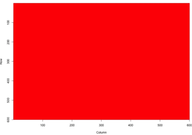
distribution{0.33,0.33,0.33}. According to our bicluster definition, it has 1 bicluster and S is the same over all columns. The number of categories of the data in Data set C was set to 3.

Figure 3.1: The true bicluster structure from which Data matrix A is simulated. Each color demonstrates a di↵erent bicluster. Each of the 3 biclusters contains 200 rows and 800 columns.

(52)

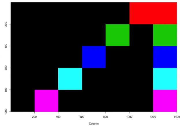
Figure 3.2: The true structure for Data matrix B. There are 5 biclusters embedded, with an equal size 200 by 400.

(53)

Figure 3.3: The true structure for Data matrix C. The data are generated randomly for each category. It corresponds to 1 background bicluster in our definition

Notice that in the first data set, there are a total of 23 _{3 = 5 distinctive patterns}

that S can take and we embed all those patterns into the data, as seen in Figure 3.1. In the second data set, there are a total of 25 _{5 = 27 distinctive patterns}_S _{can take}

and we embeded 7 of them, which is displayed in Figure 3.2. In the thrid data set,S

(54)

3.4.3 Data set A: 3 clusters

Following the sampling procedure presented in section 3.3.5, we started with 3 clusters and let the algorithm run for 1,000 steps and discard the initial 500 steps as burn-in. The priors were set as ↵z = {1,1,1}, ↵✓ = {2,2,2,2}, a = 0.05. The

initial values forZ,S, and⇥were assigned randomly based on their priors. The trace plot of joint posteriors for all 3 chains can be viewed in Figure 3.4. We can see that chain 2 was trapped in local mode. To further investigate, we increased the number of independent chains to 100 and found out that 11 of the chains were stuck in local modes.

(55)

Figure 3.4: Trace plot for the joint posteriors of 3 independent chains. Chain 2 is plotted in red.

(56)

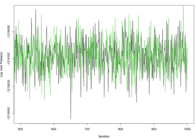
Figure 3.5: Trace plot for the joint posteriors of the chain 1 and 2, after burn-in.

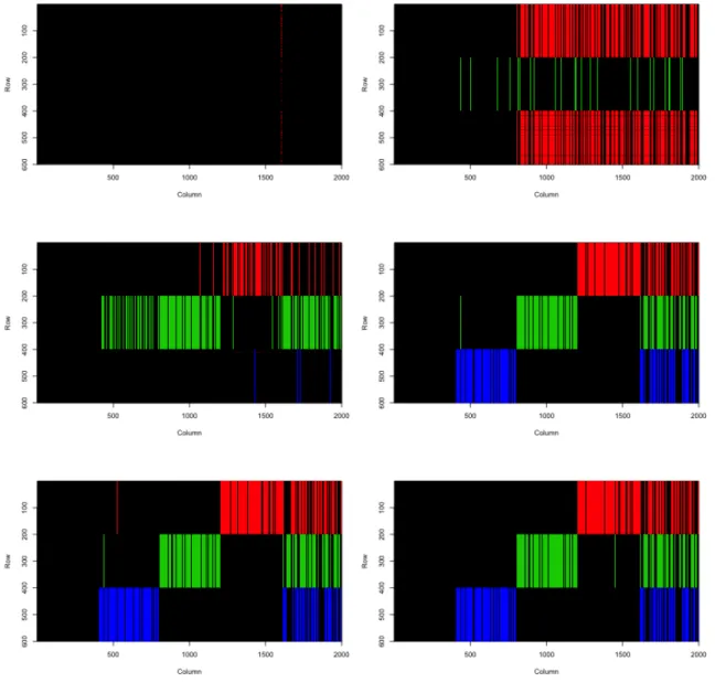
By looking into chain 1 which is not in a local mode, we can plot the recovered bicluster structure as the iteration goes in Figure 3.6. The bicluster structure in the plots correspond to those at step 20, 22, 25, 27, 50, 80. We can see the algorithm converges to the truth very fast even starting from random initial values.

(57)

Figure 3.6: Recovered bicluster structure at di↵erent step.

As a solution to the local mode trapping problem, we chose the chains with highest joint posteriors and plotted their mixing after burn-in in Figure 3.5. As we can see, the mixing is good. Then we started with 2, 4, 5, 6 clusters, each with 10 independent chains and found out that all these independent runs will eventually converge to 3 or

(58)

2 clusters. We compared their joint posterior modes from corresponding chains with highest posteriors and found that the optimal number of clusters in this simulated was 3.

An alternative approach to overcome the local mode problem is to use a hierar-chical clustering method to provide a starting configuration for our algorithm. More precisely, we treated the categorical data as continuous and employed the Euclidean distance measure for hiearchical clustering.

We again ran 3 parallel MCMC chains with ↵z = {1,1,1}, ↵✓ = {2,2,2,2}, a= 0.05. The initial values forZ were set using the results from hierarchical clustering and it converges very fast. The diagnostics for the parallel chains are presented in Figure 3.7 and 3.8. The ACF plot in Figure 3.9 reveals that the autocorrelation drops to 0 at a high rate. The implementation of hierarchical clustering was adapted from open source clustering package Cluster 3.0. (de Hoon et al. (2004))

(59)

Figure 3.7: Trace plot for the joint posteriors of 3 independent chains, started with hierarchical clustering results.

(60)

Figure 3.8: Trace plot for the joint posteriors of 3 independent chains after burn-in, started with hierarchical clustering results.

(61)

Figure 3.9: ACF plot for the joint posteriors, started with hierarchical clustering results

By running the algorithm with 3, 4, 5, and 6 clusters, the algorithm will all converge to 3 clusters as the iterations run. However, if we started with 2 clusters, the algorithm will stay at 2 because of the high energy barrier. After comparing the joint posterior mode at 2 and 3 clusters, we finally identified 3 as the optimal number of clusters, which is consistent with the true number of clusters. The change of number of clusters from di↵erent runs is illustrated in Figure 3.10.

(62)

Figure 3.10: Change of number of clusters from independent runs starting from 2, 3, 4, 5, 6 clusters

The results of the recovered biclustering structure is plotted in Figure 3.11. The Jaccard Index for this estimate is 0.87, which indicates a good estimate of the original biclustering structure. Di↵erent reasonable settings of priors have also be tested and they have little impact on the estimation accuracy. A detailed comparision of the sensitivity of the algorithm is presented at the end of this Chapter.

(63)

Figure 3.11: the biclusters learned through the MCMC algorithm. They resemble the true structure in general except for a small amount of errors.

3.4.4 Data set B: 5 clusters

We performed similar analysis for Data matrix 2, started with 2, 3, 4, 5, 6, 7, and 8 clusters independently, and the number of clusters converged to 5 when greater than 5. By comparing their joint posterior mode we chose 5 as the optimal number of clusters. The diagnostic plots are presented as in Figure 3.12 and Figure 3.13.

(64)

(65)

Figure 3.13: Autocorrelation plot for the joint posterior for 5 clusters. No significant autocorrelation emerges when the lag is greater than 1.

(66)

Figure 3.14: The 5 biclusters determined by joint posterior mode. The estimated bicluster structure is very close to the true structure.

The estimated biclustering structure is presented in Figure 3.14. The recovered structure is very similar to the embeded true bicluster structure with a Jaccard Index of 0.86.

3.4.5 Data set C: 1 cluster

For Data set C, we let the algorithm run starting from 1, 2, 3, 4, 5, 6 clusters and it all converges to 1 bicluster, which is the same as we simulated.

(67)

3.4.6 Sensitivity tests for Bayesian Categorical BiClustering

Model

In this section, we will present the experiments we performed to test the sensitiv-ity of the Bayesian Categorical Biclustering algorithm. To test the sensitivsensitiv-ity of the algorithm, we embeded 3 biclusters into the data as in Figure 3.1, each with di↵ er-ent similarities between the column bicluster specific multinomial distributions. The number of categories of data was set to be 3. In the simulated data, the same color in each column means the data was drawing from the same multinomial distribution. Di↵erent colors on the same column means that they are each from a di↵erent multi-nomial distribution. All the multimulti-nomial distributions were generated from the same prior Dirichlet distribution.

As↵increases, the sampled probability vectors for column bicluster-specific multi-nomial distributions, fromDirichlet(↵,↵, . . . ,↵) will tend to be more and more sim-ilar to each other. We let ↵ go from 0.1 to 10 and calculated the estimate accuracy by evaluating the Jaccard Index for each simulation. In our Gibbs sampling, we used the same prior setting (↵z = 1, ↵p = 2 and a = 0.1) across all tests. The recovered

(68)

Table 3.1: Sensitivity Test Results

Dirichlet Prior: ↵ a ↵z ↵p Jaccard Index

(0.1, 0.1, 0.1) 0.1 1 2 0.779 (0.2, 0.2, 0.2) 0.1 1 2 0.833 (0.3, 0.3, 0.3) 0.1 1 2 0.849 (0.4, 0.4, 0.4) 0.1 1 2 0.846 (0.5, 0.5, 0.5) 0.1 1 2 0.843 (1, 1, 1) 0.1 1 2 0.802 (5, 5, 5) 0.1 1 2 0.601 (7, 7, 7) 0.1 1 2 0.330 (10, 10, 10) 0.1 1 2 0.137

As we can see, when the Dirichlet prior for generating the data goes beyond 5, the estimate accuracy drops fast and becomes unsatisfactory. The algorithm is in general very robust. We tried di↵erent values for↵z and ↵p in our sampling and the

recovered bicluster structure and Jaccard Index accuracy are similar. There are lots of potential applications of this algorithm in real life and we hope it can help facilitate new scientific discoveries.

(69)

Figure 3.15: Bicluster structure learned through the MCMC algorithm. All column bicluster specific multinomial parameters are drawn fromDirichlet(0.1,0.1,0.1). Jac-card Index: 0.779

(70)

(71)

(72)

(73)

(74)

Figure 3.20: Bicluster structure learned through the MCMC algorithm. All column bicluster specific multinomial parameters are drawn from Dirichlet(1,1,1). Jaccard Index: 0.802

(75)

(76)

(77)

Figure 3.23: Bicluster structure learned through the MCMC algorithm. All column bicluster specific multinomial parameters are drawn from Dirichlet(10,10,10). Jac-card Index: 0.137

(78)

Chapter 4 Bayesian Biclustering on Ordinal

Data

4.1 Introduction

Ordinal data is a statistical data type we see often in real life. For example, in movie rating websites like Internet Movie Database (IMDB), people are asked to rate a movie on a scale of 1 to 5. A rating of 5 stars is better than a 4 star rating, but we do not know how much better it is. Ordinal data captures the ordering information in the data and presents it as discrete values. The intervals between successive scales are usually not equal. We also see this type of data in questionnaires, reviews etc. Another everyday example is the Apple App store, which asks people to rate the apps they downloaded on an ordinal scale of up to 5 stars.

As we discussed in Chapter 1, a certain type of bicluster with coherent evaluation patterns consists of orders instead of the real numerical values of the data. Taking

(79)

Chapter 4: Bayesian Biclustering on Ordinal Data

movie rating data, for example, we are interested in finding individuals such that their ratings are more similar to each other, over a subset of movies. After finding those cliques, we can build a recommendation system for suggesting movies to users. We have not been able to find existing biclustering methods for ordinal data. We here propose two Bayesian Biclustering algorithms, one using latent variable and cuto↵ points from the normal distribution to model ordinal data, and the other one using a mixture of binomial and discrete uniform distributions. There are more parameters in the normal cuto↵ model when levels of data are higher, while the intuition behind the modeling is more straightforward. The mixture model uses a fixed number of two parameters for each bicluster and is easier in terms of implementation and converges faster. In the following sections, we will first illustrate the Bayesian modeling of Uniform Binomial Mixture model (UBM) and test the model with a simulated data set. The Normal Random Cuto↵model (NRC) will be discussed later and the general framework will be presented at the end of this chapter.

Bayesian Biclustering on Discrete Data: Variable Selection Methods

Bayesian Biclustering on Discrete Data: Variable Selection

Methods

(Article begins on next page)

The Harvard community has made this article openly available.

Please share

how this access benefits you. Your story matters.

Citation

Guo, Lei. 2013. Bayesian Biclustering on Discrete Data: Variable

Selection Methods. Doctoral dissertation, Harvard University.

Accessed

Citable Link

http://nrs.harvard.edu/urn-3:HUL.InstRepos:11181216

Terms of Use

This article was downloaded from Harvard University's DASH

repository, and is made available under the terms and conditions

applicable to Other Posted Material, as set forth at

http://nrs.harvard.edu/urn-3:HUL.InstRepos:dash.current.terms-of-use#LAA

Bayesian Biclustering on Discrete Data: Variable

Selection Methods

Bayesian Biclustering on Discrete Data: Variable Selection

Methods

Abstract

Contents

Acknowledgments

Chapter 1

Introduction

Chapter 2

An overview of Biclustering

Methods

2.1

Notation

2.2

Types of Biclusters

2.3

Patterns of Biclusters

2.4

Biclustering algorithms

Chapter 3

Bayesian Biclustering on

Categorical Data

3.1

Background

3.2

Categorical Data

3.3

Modeling

3.3.1

Notations

3.3.2

Model Settings

3.3.3

Sampling Methods

3.3.4

Determination of Number of Clusters

3.3.5

Algorithm Summary

3.4

Simulation Study

3.4.1

Validation of Biclustering Results

3.4.2

Date Generation

3.4.3

Data set A: 3 clusters

3.4.4

Data set B: 5 clusters

3.4.5

Data set C: 1 cluster

3.4.6

Sensitivity tests for Bayesian Categorical BiClustering

Model

Chapter 4

Bayesian Biclustering on Ordinal

Data

4.1

Introduction

_{Selection Methods. Doctoral dissertation, Harvard University.}

_{repository, and is made available under the terms and conditions}