ROSE: A Package for Binary Imbalanced
Learning
by Nicola Lunardon, Giovanna Menardi, and Nicola Torelli
Abstract TheROSEpackage provides functions to deal with binary classification problems in the presence of imbalanced classes. Artificial balanced samples are generated according to a smoothed bootstrap approach and allow for aiding both the phases of estimation and accuracy evaluation of a binary classifier in the presence of a rare class. Functions that implement more traditional remedies for the class imbalance and different metrics to evaluate accuracy are also provided. These are estimated by holdout, bootstrap, or cross-validation methods.
Introduction
Imbalanced learningis the heading which denotes the problem of supervised classification when one of the classes is rare over the sample. As class imbalance situations are pervasive in a plurality of fields and applications, the issue has received considerable attention recently. Numerous works have focused on warning about the heavy implications of neglecting the imbalance of classes, as well as proposing suitable solutions to relieve the problem. Nonetheless, there is a general lack of procedures and software explicitly aimed at handling imbalanced data and which can be readily adopted also by non expert users. To the best of our knowledge, in the R environment, only a few functions are designed for imbalanced learning. It is worth mentioning packageDMwR(Torgo,2010), which provides a specific function (smote) to aid the estimation of a classifier in the presence of class imbalance, in addition to extensive tools for data mining problems (among others, functions to compute evaluation metrics as well as different accuracy estimators). In addition, packagecaret(Kuhn,2014) contains general functions to select and validate regression and classification problems and specifically addresses the issue of class imbalance with some naive functions (downSampleandupSample).
These reasons motivate theROSEpackage (Lunardon et al.,2013), which is intended to provide both standard and more refined tools to enhance the task of binary classification in an imbalanced setting. The package is designed around ROSE (Random Over-Sampling Examples), a smoothed bootstrap-based technique which has been recently proposed byMenardi and Torelli(2014). ROSE helps to relieve the seriousness of the effects of an imbalanced distribution of classes by aiding both the phases of model estimation and model assessment.
This paper is organized as follows: after a brief introduction to the problem of class imbalance and to the statistical foundations at the basis of the ROSE method, we provide an overview of the functions included in the package and illustrate their use with a numerical example.
The class imbalance problem
Without attempting a full discussion, we summarize here the main statistical issues emerging in imbalanced learning. The outline focuses on those aspects that are relevant for a full comprehension of the routines implemented in the package. The interested reader is invited to refer toMenardi and Torelli(2014) and the references therein for a deeper discussion and technical details.
The presence of a strong imbalance in the distribution of the response variable may lead to heavy consequences in pursuing a classification task, in both phases of model estimation and accuracy evalu-ation. Disregarding the specificities of different models, what typically happens is that classification rules are overwhelmed by the prevalent class and the rare examples are ignored.
Most of the current research on imbalanced classification focuses on proposing solutions to improve the model estimation step. The most common remedy to the imbalance problem involves altering the class distribution to obtain a more balanced sample. Remedies based on balancing the class distribution include various techniques of data resampling, such as random oversampling (with replacement) of the rare class and random undersampling (without replacement) of the prevalent class. Under the same hat of these balancing methods, we can also include the ones designed to generate new artificial examples that are ‘similar’, in a certain sense, to the rare observations. Generation of new artificial data that have not been previously observed reduces the risk of overfitting and improves the ability of generalization compromised by oversampling methods, which are bound to produce ties in the sample. As will be clarified subsequently, the ROSE technique can be rightly considered as following this route.
is at least as important as model estimation, because the extent to which a classification rule may be operationally applied to real-world problems, for labeling new unobserved examples, depends on our ability to measure classification accuracy.
In the accuracy evaluation step, the first problem one has to face concerns the choice of the accuracy metric, since the use of standard measures, such as the overall accuracy, may yield misleading results. The choice of the evaluation measure has to be addressed in terms of some class-independent quantities, such as precision, recall or the F measure. For the operational computation of these measures, one should set a suitable threshold for the probability of belonging to the positive class, above which an example is predicted to be positive. In standard classification problems, this threshold is usually set to 0.5, but the same choice is not obvious in imbalanced learning, as it is likely that no examples are labeled as positive. Moreover, moving a threshold to smaller values is equivalent to assume a higher misclassification cost for the rare class, which is usually the case. To avoid an arbitrary choice of the threshold, a ROC curve can be adopted to measure the accuracy, because it plots the true positive rate versus the false positive rate as the classification threshold varies.
Apart from the choice of an adequate performance metric, a more serious problem in imbalanced learning concerns the estimation method for the selected accuracy measure. To this aim, standard practices are the resubstitution method, where the available data are used for both training and assessing the classifier or, more frequently, the holdout method, which consists of estimating the classifier over a training sample of data and assessing its accuracy on a test sample. In the presence of a class imbalance, often, there are not sufficient examples from the rare class for both training and testing the classifier. Additionally, the scarcity of data leads to estimates of the accuracy measure which are affected by a high variance and are then regarded as unreliable. On the other hand, the resubstitution method is known to lead to overoptimistic evaluation of learner accuracy. Then, alternative estimators of the accuracy measure have to be considered, as pointed out in the next section.
The ROSE strategy to deal with class imbalance
ROSE (Menardi and Torelli,2014) provides a unified framework to deal simultaneously with the two above-mentioned problems of model estimation and accuracy evaluation in imbalanced learning. It builds on the generation of new artificial examples from the classes, according to a smoothed bootstrap approach (see,e.g., Efron and Tibshirani,1993).
Consider a training setTn, of sizen, whose generic row is the pair(xi,yi),i=1, . . . ,n. The class
labelsyibelong to the set{Y0,Y1}, andxiare some related attributes supposed to be realizations of a
random vectorxdefined on Rd, with an unknown probability density functionf(x). Let the number of units in classYj,j=0, 1, be denoted bynj<n. The ROSE procedure for generating one new artificial
example consists of the following steps: 1. Selecty∗=Yjwith probabilityπj.
2. Select(xi,yi)∈Tn, such thatyi=y∗, with probabilityn1j.
3. Samplex∗ fromKHj(·,xi), withKHj a probability distribution centered atxi and covariance
matrixHj.
Essentially, we draw from the training set an observation belonging to one of the two classes, and gen-erate a new example(x∗,y∗)in its neighborhood, where the shape of the neighborhood is determined by the shape of the contour sets ofKand its width is governed byHj.
It can be easily shown that, given selection of the class labelYj, the generation of new examples fromYj, according to ROSE, corresponds to the generation of data from the kernel density estimate of f(x|Yj), with kernelKand smoothing matrixHj(Menardi and Torelli,2014). The choices ofKand
Hjmay be then addressed by the large specialized literature on kernel density estimation (see,e.g.
Bowman and Azzalini,1997). It is worthwhile to note that, forHj→0, ROSE collapses to a standard
combination of over- and under-sampling.
Repeating steps 1 to 3mtimes produces a new synthetic training setT∗m, of sizem, where the
imbalance level is defined by the probabilitiesπj(ifπj=1/2, then approximately the same number of
examples belong to the two classes). The sizemmay be set to the original training set sizenor chosen in any way.
Apart from enhancing the process of learning, the synthetic generation of new examples from an estimate of the conditional densities of the two classes may also aid the estimation of learner accuracy and overcome the limits of both resubstitution and the holdout method. Operationally, the use of ROSE for estimating learner accuracy may follow different schemes, which resemble standard accuracy estimators but claim a certain degree of originality. For example, a holdout version of ROSE would involve testing the classifier on the originally observed data after training it on the artificial training setT∗m. Alternatively, bootstrap or cross-validated versions of ROSE may be chosen as estimation
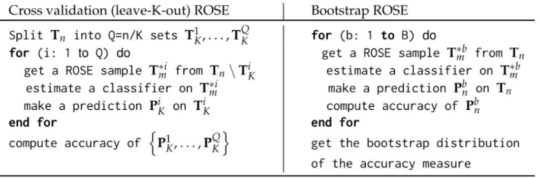
Table 1:Pseudo-code of the alternative uses of ROSE for model assessment.
Cross validation (leave-K-out) ROSE Bootstrap ROSE Split Tn into Q=n/K sets T1K, . . . ,T
Q
K for (b: 1 to B) do
for (i: 1 to Q) do get a ROSE sample T∗mb from Tn
get a ROSE sample T∗mi from Tn\TiK estimate a classifier on T∗mb
estimate a classifier on T∗mi make a prediction Pbn on Tn
make a prediction PiK on TiK compute accuracy of Pbn
end for end for
compute accuracy of nP1K, . . . ,PQKo get the bootstrap distribution of the accuracy measure
methods, as illustrated in Table1. An extensive simulation study inMenardi and Torelli(2014) has, in fact, shown that the holdout and bootstrap versions of ROSE tend to overestimate the accuracy, but their mean square error is lower than the one obtained by utilizing a standard holdout method. Hence, overall, these estimates are preferable.
Package illustration
Overview
The package provides a complete toolkit to tackle the problem of binary classification in the presence of imbalanced data. Functions are supplied to encompass all phases of the learning process: from model estimation to assessment of the accuracy of the classification. In the former phase, the user has to choose both the remedy to adopt for the class imbalance, and the classifier to estimate for the learning process. For the first aim, functionsROSEorovun.samplecan be adopted to balance the sample. One is allowed to choose among all the functions already implemented in R to build the desired binary classifier, such asglm,rpart,nnet, as well as user defined functions. Once a classifier has been trained, its accuracy has to be evaluated, which requires the choice of both an appropriate accuracy measure, and an estimation method that can provide a reliable estimate of such measure. Functionsroc.curveandaccuracy.measimplement the most commonly adopted measures of accuracy in imbalance learning, while functionROSE.evalprovides a ROSE version of holdout, bootstrap or cross-validation estimates of the accuracy measures, as described above.
A summary of the functions provided by the package, classified according to the main tasks they are designed for, is listed in Table2.
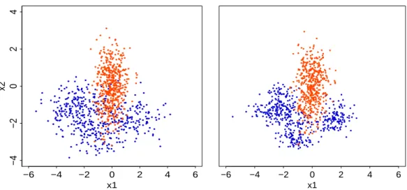
ROSEalso includes the simulated datahacide, which are adopted here to illustrate the pack-age. The workspacehacideconsists of a bidimensional training sethacide.trainand a test set hacide.test, amounting to 1000 and 250 rows, respectively. The binary label class (denoted ascls) has a heavily imbalanced distribution, with the positive examples occurring in approximately 2% of the cases. The rare class may be described as a depleted noisy semi-circle filled with the prevalent class, which is normally distributed and has elliptical contours. See the top-left panel of Figure1for an illustration.
Ignoring the imbalance
After loading the package and the data, we explore the training set structure: > library(ROSE)
Loaded ROSE 0.0-3
Table 2:Summary of the functions in packageROSE
Data balancing
ROSE
ovun.sample
Accuracy measures
roc.curve accuracy.meas
Accuracy estimatorsROSE.eval
x2 −4 −2 0 2 4 ● ● ● ● ● ● ● ● ● ● ● ● ● ● ● ● ● ● ● ● ● ● ● ● ● ● ● ● ● ● ● ● ● ● ● ● ● ● ● ● ● ● ● ● ● ● ● ● ● ● ● ● ● ● ● ● ● ● ● ● ● ● ● ● ● ● ● ● ● ● ● ● ● ● ● ● ● ● ● ● ● ● ● ● ● ● ● ● ● ● ● ● ● ● ● ● ● ● ● ● ● ● ● ● ● ● ● ● ● ● ● ● ● ● ● ● ● ● ● ● ● ● ● ● ●● ● ● ● ● ● ● ● ● ● ● ● ● ● ● ● ● ● ● ● ● ● ● ● ● ● ● ● ● ● ● ● ● ● ● ● ● ● ● ● ● ● ● ● ● ● ● ● ● ● ● ● ● ● ● ● ● ● ● ●● ● ● ● ● ● ● ● ● ● ● ● ● ● ● ● ● ● ● ● ● ● ● ● ● ● ● ● ● ● ● ● ● ● ● ● ● ● ● ● ● ● ● ● ● ● ● ● ● ● ● ● ● ● ● ● ● ● ● ● ● ●● ● ● ● ● ● ● ● ● ● ● ● ● ● ● ● ● ● ● ● ● ● ● ● ● ● ● ● ● ● ● ● ● ● ● ● ● ● ● ● ● ● ● ● ● ● ● ● ● ● ● ● ● ● ● ● ● ● ● ● ● ● ● ● ● ● ● ● ● ● ● ● ● ● ● ● ● ● ● ● ● ● ● ● ● ● ● ● ● ● ● ● ● ● ● ● ● ● ● ● ● ● ● ● ● ● ● ● ● ● ● ● ● ● ● ● ● ● ● ● ● ● ● ● ●● ● ● ● ● ● ● ● ● ● ● ● ● ● ● ● ● ●● ● ● ● ● ● ● ● ● ● ● ● ● ● ● ● ● ● ● ● ● ● ● ● ● ● ● ● ● ● ● ● ● ● ● ● ● ● ● ● ● ● ● ● ● ● ● ● ●● ● ● ● ● ● ● ● ● ● ● ● ● ● ● ● ● ● ● ● ● ● ● ● ● ● ● ● ● ● ●●● ● ● ● ● ● ● ● ● ● ● ● ● ● ● ● ● ● ● ● ● ● ● ● ● ● ● ● ● ● ● ● ● ● ● ● ● ● ● ● ● ● ● ● ● ● ● ● ● ● ● ● ● ● ● ● ● ● ● ● ● ● ● ● ● ● ● ● ● ● ● ● ● ● ● ● ● ● ● ● ● ● ● ● ● ● ● ● ● ● ● ● ● ● ● ● ● ● ● ● ● ● ● ● ● ● ● ● ● ● ● ● ● ● ● ● ● ● ● ● ● ● ● ● ● ● ● ● ● ● ● ● ● ● ● ● ● ● ● ● ● ● ● ● ● ● ● ● ● ● ● ● ● ● ● ● ● ● ● ● ● ● ● ● ● ● ● ● ● ● ● ● ● ● ● ● ● ● ● ● ● ● ● ● ● ● ● ● ● ● ● ● ● ● ● ● ● ● ● ● ● ● ● ● ● ● ● ● ● ● ● ● ● ● ● ● ● ● ● ● ● ● ● ● ● ● ● ● ● ● ● ● ● ● ● ● ● ● ● ● ● ● ● ● ● ● ● ● ● ● ● ● ● ● ● ● ● ● ● ● ● ● ● ● ● ● ● ● ● ● ● ● ● ● ● ● ● ● ● ● ● ● ● ● ● ● ● ● ● ● ● ● ● ● ● ● ● ● ● ● ● ● ● ● ● ● ● ● ● ● ● ● ● ● ● ● ● ● ● ● ● ● ● ● ● ● ● ● ● ● ● ● ● ● ● ● ● ● ● ● ● ● ● ● ● ● ● ● ● ● ● ● ● ● ● ● ● ● ● ● ● ● ● ● ● ● ● ● ● ● ● ● ● ● ● ● ● ● ● ● ● ● ● ● ● ● ● ● ● ● ● ● ● ● ● ● ● ● ● ● ●● ● ● ● ● ● ● ● ● ● ● ● ● ● ● ● ● ● ● ● ● ● ● ● ● ● ● ● ● ● ● ● ● ● ● ●● ● ● ● ● ● ● ● ● ● ● ● ● ● ● ● ● ● ● ● ● ● ● ● ● ● ● ● ● ● ● ● ● ● ● ● ● ● ● ● ● ● ● ● ● ● ● ● ● ● ● ● ● ● ● ● ● ● ● ● ● ● ● ● ● ● ● ● ● ● ● ● ● ● ● ● ● ● ● ● ● ● ● ● ● ● ● ● ● ● ● ● ● ● ● ● ● ● ● ● ● ● ● ● ● ● ● ● ● ● ● ● ● ● ● ● ● ● ● ● ● ● ● ● ● ● ● ● ● ● ● ● ● ● ● ● ● ● ● ● ● ● ● ● ● ● ● ● ● ● ● ● ● ● ● ● ● ● ● ● ● ● ● ● ● ● ● ● ● ● ● ● ● ● ● ● ● ● ● ● ● ● ● ● ● ● ● ● ● ● ● ● ● ● ● ● ● ● ● ● ● ● ● ● ● ● ● ● ● ● ● ● ● ● ● ● ● ● ● ● ● ● ● ● ● ● ● ● ● ● ● ● ● ● ● ● ●● ● ● ● ● ● ● ● ● ● ● ● ● ● ● ● ● ● ● ● ● ● ● ● ● ● ● ● ● ● ● ● ● ● ● ● ● ● ● ● ● ● ● ● ● ● ● ● ● ● ● ● ● ● ● ● ● ● ● ●● ● ● ● ● ● ● ● ● ● ● ● ● ● ● ● ● ● ● ● ● ● ● ● ● ● ● ● ● ● ● ● ● ● ● ● ● ● ● ● ● ● ● ● ● ● ● ● ● ● ● ● ● ● ● ● ● ● ● ● ● ●● ● ● ● ● ● ● ● ● ● ● ● ● ● ● ● ● ● ● ● ● ● ● ● ● ● ● ● ● ● ● ● ● ● ● ● ● ● ● ● ● ● ● ● ● ● ● ● ● ● ● ● ● ● ● ● ● ● ● ● ● ● ● ● ● ● ● ● ● ● ● ● ● ● ● ● ● ● ● ● ● ● ● ● ● ● ● ● ● ● ● ● ● ● ● ● ● ● ● ● ● ● ● ● ● ● ● ● ● ● ● ● ● ● ● ● ● ● ● ● ● ● ● ● ●● ● ● ● ● ● ● ● ● ● ● ● ● ● ● ● ● ●● ● ● ● ● ● ● ● ● ● ● ● ● ● ● ● ● ● ● ● ● ● ● ● ● ● ● ● ● ● ● ● ● ● ● ● ● ● ● ● ● ● ● ● ● ● ● ● ●● ● ● ● ● ● ● ● ● ● ● ● ● ● ● ● ● ● ● ● ● ● ● ● ● ● ● ● ● ● ●●● ● ● ● ● ● ● ● ● ● ● ● ● ● ● ● ● ● ● ● ● ● ● ● ● ● ● ● ● ● ● ● ● ● ● ● ● ● ● ● ● ● ● ● ● ● ● ● ● ● ● ● ● ● ● ● ● ● ● ● ● ● ● ● ● ● ● ● ● ● ● ● ● ● ● ● ● ● ● ● ● ● ● ● ● ● ● ● ● ● ● ● ● ● ● ● ● ● ● ● ● ● ● ● ● ● ● ● ● ● ● ● ● ● ● ● ● ● ● ● ● ● ● ● ● ● ● ● ● ● ● ● ● ● ● ● ● ● ● ● ● ● ● ● ● ● ● ● ● ● ● ● ● ● ● ● ● ● ● ● ● ● ● ● ● ● ● ● ● ● ● ● ● ● ● ● ● ● ● ● ● ● ● ● ● ● ● ● ● ● ● ● ● ● ● ● ● ● ● ● ● ● ● ● ● ● ● ● ● ● ● ● ● ● ● ● ● ● ● ● ● ● ● ● ● ● ● ● ● ● ● ● ● ● ● ● ● ● ● ● ● ● ● ● ● ● ● ● ● ● ● ● ● ● ● ● ● ● ● ● ● ● ● ● ● ● ● ● ● ● ● ● ● ● ● ● ● ● ● ● ● ● ● ● ● ● ● ● ● ● ● ● ● ● ● ● ● ● ● ● ● ● ● ● ● ● ● ● ● ● ● ● ● ● ● ● ● ● ● ● ● ● ● ● ● ● ● ● ● ● ● ● ● ● ● ● ● ● ● ● ● ● ● ● ● ● ● ● ● ● ● ● ● ● ● ● ● ● ● ● ● ● ● ● ● ● ● ● ● ● ● ● ● ● ● ● ● ● ● ● ● ● ● ● ● ● ● ● ● ● ● ● ● ● ● ● ● ● ● ● ●● ● ● ● ● ● ● ● ● ● ● ● ● ● ● ● ● ● ● ● ● ● ● ● ● ● ● ● ● ● ● ● ● ● ● ●● ● ● ● ● ● ● ● ● ● ● ● ● ● ● ● ● ● ● ● ● ● ● ● ● ● ● ● ● ● ● ● ● ● ● ● ● ● ● ● ● ● ● ● ● ● ● ● ● ● ● ● ● ● ● ● ● ● ● ● ● ● ● ● ● ● ● ● ● ● ● ● x1 x2 ● ● ● ● ● ● ● ● ● ● ● ● ● ● ● ● ● ● ● ● ● ● ● ● ● ● ● ● ● ● ● ● ●● ● ● ● ● ● −6 −4 −2 0 2 4 6 −4 −2 0 2 4 x1 ● ● ● ● ● ● ●● ● ● ● ● ● ● ● ● ● ● ● ● ● ● ● ● ● ● ● ● ● ● ● ● ● ● ● ● ● ● ● ● ● ● ● ● ● ● ● ● ● ● ● ● ● ● ● ● ● ● ● ● ● ● ● ● ● ● ● ● ● ● ● ● ● ● ● ● ● ● ● ● ● ● ● ● ● ● ● ● ● ● ● ● ● ● ● ● ● ● ● ● ● ● ● ● ● ● ● ● ● ● ● ● ● ● ● ● ● ● ● ● ● ● ● ● ● ● ● ● ● ● ● ● ●● ● ● ● ●● ● ● ● ● ● ● ● ● ● ● ● ● ● ● ● ● ● ● ● ● ●● ● ● ● ● ● ● ● ● ● ● ● ● ● ● ● ● ● ● ● ● ● ● ● ● ● ● ● ● ● ● ● ● ● ● ● ● ● ● ● ● ● ● ● ● ● ● ● ● ● ● ● ● ● ● ● ● ● ● ● ● ● ● ● ● ● ● ● ● ● ● ● ● ● ● ● ● ● ● ● ● ● ● ● ● ● ● ● ● ● ● ● ● ● ● ● ● ● ● ● ● ● ● ● ● ● ● ● ● ● ● ● ● ● ● ● ● ● ● ● ● ● ● ● ● ● ● ● ● ● ● ● ● ● ● ● ● ● ● ● ● ● ● ● ● ● ● ● ● ● ● ● ● ● ● ● ● ● ● ● ● ● ● ● ● ● ● ● ● ● ● ● ● ● ● ● ● ● ● ● ● ● ● ● ● ● ● ● ● ● ● ● ● ● ● ● ● ● ● ● ● ● ● ● ● ● ● ● ● ● ● ● ● ● ● ● ● ● ● ● ● ● ● ● ● ● ● ● ● ● ● ● ● ● ● ● ● ● ● ● ● ● ● ● ● ● ● ● ● ● ● ● ● ● ● ● ● ● ● ● ● ● ● ● ● ● ● ● ● ● ● ● ● ● ● ● ● ● ● ● ● ● ● ● ● ● ● ● ● ● ● ● ● ● ● ● ● ● ● ● ● ● ●● ● ● ● ● ● ● ● ● ● ● ● ● ● ● ● ● ● ● ● ● ● ● ● ● ● ● ● ● ● ● ● ● ● ● ● ● ● ● ● ● ● ● ● ● ● ● ● ● ● ● ●● ● ● ● ● −6 −4 −2 0 2 4 6
Figure 1: Outcomes of data balancing strategies implemented in the ROSE package on the hacide.traindata. The orange and blue colors denote the majority and minority class examples, respectively. Top-left panel: training data; top-right: oversampling; bottom-left: undersampling; bottom-right: combination of over and undersampling.
> data(hacide) > str(hacide.train)
'data.frame': 1000 obs. of 3 variables:
$ cls: Factor w/ 2 levels "0","1": 1 1 1 1 1 1 1 1 1 1 ... $ x1 : num 0.2008 0.0166 0.2287 0.1264 0.6008 ... $ x2 : num 0.678 1.5766 -0.5595 -0.0938 -0.2984 ... > table(hacide.train$cls) 0 1 980 20
Now, we show that ignoring class imbalance is not inconsequential. Suppose we want to build a binary classification tree, based on the training data. We first load packagerpart.
> library(rpart)
> treeimb <- rpart(cls ~ ., data = hacide.train)
In the current example, the accuracy of the estimated classifier may be evaluated by a standard application of the holdout method, because as many data as we need can be simulated from the same distribution as the training sample to test the classifier. For the sake of illustration, a test sample hacide.testis supplied by the package.
Irrespective of the performance metric used for evaluation, a prediction on the test data is first required.
> pred.treeimb <- predict(treeimb, newdata = hacide.test) > head(pred.treeimb) 0 1 1 0.9898888 0.01011122 2 0.9898888 0.01011122 3 0.9898888 0.01011122 4 0.9898888 0.01011122 5 0.9898888 0.01011122 6 0.9898888 0.01011122
The accuracy may be now assessed by means of the performance metricsaccuracy.measorroc.curve provided by the package. These functions share the mandatory argumentsresponseandpredicted, representing true class labels and the predictions of the classifier, respectively. Predicted values may take the form of a vector of class labels, or alternatively may represent the probability or some score of belonging to the positive class.
> accuracy.meas(hacide.test$cls, pred.treeimb[,2]) Call:
accuracy.meas(response = hacide.test$cls, predicted = pred.treeimb[,2]) Examples are labelled as positive when predicted is greater than 0.5 precision: 1.000
recall: 0.200 F: 0.167
Functionaccuracy.meascomputes recall, precision, and the F measure. The estimated classifier shows maximum precision, that is, there are no false positives. On the other hand, recall is very low, thereby implying that the model has predicted a large number of false negatives.
Functionaccuracy.measis endowed with an optional argumentthreshold, which defines the predicted value over which an example is assigned to the rare class. As one can deduce by the the output above, argumentthresholddefaults to 0.5, like the standard cut-off probability adopted in balanced learning. In the current example, movingthresholddoes not improve classification (results not reported) but this is usually an advisable practice in imbalanced learning. Indeed, the default choice is often too high and might lead to not labeling any example as positive, which would entail undefined values for precision, recall, and F.
To safeguard the user by an arbitrary specification ofthresholdinaccuracy.meas, the package supplies functionroc.curve, which computes the area under the ROC curve (AUC) as a measure of accuracy and is not affected by the choice of any particular cut-off value.
> roc.curve(hacide.test$cls, pred.treeimb[,2], plotit = FALSE) Area under the curve (AUC): 0.600
Additionally, when optional argumentplotitis left to its defaultTRUE,roc.curvemakes an internal call toplotand displays the ROC curve in a new window. Further arguments of functionsplotand linescan be invoked inroc.curveto customize the resulting ROC curve.
In the current example, the returned AUC is small, thereby indicating that the poor prediction is due to the class imbalance and is not imputable to a wrong threshold.
Balancing the data
The example above highlights the need of adopting a cure for the class imbalance. The first-aid set of remedies provided by the package involves creation of a new artificial data set by suitably resampling the observations belonging to the two classes. Functionovun.sampleembeds some consolidated resampling techniques to perform such a task and considers different sampling schemes. It is endowed with the argumentmethod, which takes one value amongc("over","under","both").
Option"over"determines simple oversampling with replacement from the minority class until either the specified sample sizeNis reached or the positive examples have probabilitypof occurrence. Thus, whenmethod = "over", an augmented sample is returned. Since the prevalent class amounts to 980 observations, to obtain a balanced sample by oversampling, we need to set the new sample size to 1960.
> data.bal.ov.N <- ovun.sample(cls ~ ., data = hacide.train, method = "over", N = 1960)$data
> table(data.bal.ov.N$cls) 0 1
980 980
Functionovun.samplereturns an object of classlistwhose elements are the matched call, the method for data balancing, and the new set of balanceddata, which has been directly extracted here. Alterna-tively, we may design the oversampling by setting argumentp, which represents the probability of the positive class in the new augmented sample. In this case, the proportion of positive examples will be only approximatively equal to the specifiedp.
> data.bal.ov.p <- ovun.sample(cls ~ ., data = hacide.train, method = "over", p = 0.5)$data
> table(data.bal.ov.p$cls) 0 1
980 986
In general, a reader who executes this code would obtain a different distribution of the two classes, because of the randomness of the data generation. To keep trace of the generated sample, aseedmay be specified:
> data.bal.ov <- ovun.sample(cls ~ ., data = hacide.train, method = "over", p = 0.5, seed = 1)$data
The code chunks above also show how to instruct functionovun.sampleto recognize the different roles of the column data, namely through the specification of the first argumentformula. This expects the response variableclson the left-hand side and the predictors on the right-hand side, in the guise of most R regression and classification routines. As usual, the‘.’has to be interpreted as ‘all columns not otherwise in the formula’.
Similar to option"over", option"under"determines simple undersampling without replacement of the majority class until either the specified sample sizeNis reached or the positive examples has probabilitypof occurring. It then turns out that whenmethod = "under", a sample of reduced size is returned. For example, if we setp, then
> data.bal.un <- ovun.sample(cls ~ ., data = hacide.train, method = "under", p = 0.5, seed = 1)$data
> table(data.bal.un$cls) 0 1
19 20
Whenmethod = "both"is selected, both the minority class is oversampled with replacement and the majority class is undersampled without replacement. In this case, both the argumentsNandphave to be set to establish the amount of oversampling and undersampling. Essentially, the minority class is oversampled to reach a size determined as a realization of a binomial random variable with sizeNand probabilityp. Undersampling is then performed accordingly, to abide by the specifiedN.
> data.bal.ou <- ovun.sample(cls ~ ., data = hacide.train, method = "both", N = 1000, p = 0.5, seed = 1)$data
> table(data.bal.ou$cls) 0 1
520 480
From a qualitative viewpoint, these strategies produce rather different artificial data sets. A flavor of these differences is illustrated in Figure1, where the outcome of running the three options of functionovun.sample on datahacide.trainis displayed. Each observation appearing in the resulting balanced data set is represented by a point whose size is proportional to the number of ties. Oversampling produces a considerable amount of repeated observations among the rare examples, while undersampling excludes a large number of observations from the prevalent class. A combination of over- and undersampling is a compromise between the two, but still produces several ties for the minority examples when the original training set size is large and the imbalance is extreme.
Data generation according to ROSE attempts to circumvent the pitfalls of the resampling methods above by drawing a new, synthetic, possibly balanced, set of data from the two conditional kernel density estimates of the classes. Endowed with argumentsformula,data,N, andp, functionROSE shares most of its usage withovun.sample:
x1 x2 ● ● ● ● ● ● ● ● ● ● ● ● ● ● ● ● ● ● ● ● ● ● ● ● ● ● ● ● ● ● ● ● ● ● ● ● ● ● ● ● ● ● ● ● ● ● ● ● ● ● ● ● ● ● ● ● ● ● ● ● ● ● ● ● ● ● ● ● ● ● ● ● ● ● ● ● ● ● ● ● ● ● ● ● ● ● ● ● ● ● ● ● ● ● ● ● ● ● ● ● ● ● ● ● ● ● ● ● ● ● ● ● ● ● ● ● ● ● ● ● ● ● ● ● ● ● ● ● ● ● ● ● ● ● ● ● ● ● ● ● ● ● ● ● ● ● ● ● ●● ● ● ● ● ● ● ● ● ● ● ● ● ● ● ● ● ● ● ● ● ● ● ● ● ● ● ● ● ● ● ● ● ● ● ● ● ● ● ● ● ● ● ● ● ● ● ● ● ● ● ● ● ● ● ● ● ● ● ● ● ● ● ● ● ● ● ● ● ● ● ● ● ● ● ● ● ● ● ● ● ● ● ● ● ● ● ● ● ● ● ● ● ● ● ● ● ● ● ● ● ● ● ● ● ● ● ● ● ● ● ● ● ● ● ● ● ● ● ● ● ● ● ● ● ● ● ● ● ● ● ● ● ● ● ● ● ● ● ● ● ● ● ● ● ● ● ● ● ● ● ● ● ● ● ● ● ● ● ● ● ● ● ● ● ● ● ● ● ● ● ● ● ● ● ● ● ● ● ● ● ● ● ● ● ● ● ● ● ● ● ● ● ● ● ● ● ● ● ● ● ● ● ● ● ● ● ● ● ● ● ● ● ● ● ● ● ● ● ● ● ●● ● ● ● ● ● ● ● ● ● ● ● ● ● ● ● ● ● ● ● ● ● ● ● ● ● ● ● ● ● ● ● ● ● ● ● ● ● ● ● ● ● ● ● ● ● ● ● ● ● ● ● ● ● ● ● ● ● ● ● ● ● ● ● ● ● ● ● ● ● ● ● ● ● ● ● ● ● ● ● ● ● ● ● ● ● ● ● ● ● ● ● ● ● ● ● ● ● ● ● ● ● ● ● ● ● ● ● ● ● ● ● ● ● ● ● ● ● ● ● ● ● ● ● ● ● ●● ● ● ● ●● ● ● ● ● ● ● ● ● ● ● ● ● ● ● ● ● ● ● ● ● ● ● ● ● ● ● ● ● ● ● ● ● ● ● ● ● ● ● ● ● ● ● ● ● ● ●● ● ● ● ● ● ● ● ● ● ● ● ● ● ● ● ● ● ● ● ● ● ● ● ● ● ● ● ● ● ● ● ● ● ● ● ● ●● ● ● ● ● ● ● ● ● ● ● ● ● ● ● ● ● ● ● ● ● ● ● ● ● ● ● ● ● ● ● ● ● ● ● ● ● ● ● ● ● ● ● ● ● ● ● ● ● ● ● ● ● ● ● ● ● ● ● ● ● ● ● ● ● ● ● ● ● ● ● ● ● ● ● ● ● ● ● ● ● ● ● ● ● ● ● ● ● ● ● ● ● ● ● ● ● ● ● ● ● ● ● ● ● ● ● ● ● ● ● ● ● ● ● ● ● ● ● ● ● ● ● ● ● ● ● ● ● ● ● ● ● ● ● ● ● ● ● ● ● ● ● ● ● ● ● ● ● ● ● ● ● ● ● ● ● ● ● ● ● ● ● ● ● ● ● ● ● ● ● ● ● ● ● ● ● ● ● ● ● ● ● ● ● ● ● ● ● ● ● ● ● ● ● ● ● ● ● ● ● ● ● ● ● ● ● ● ● ● ● ● ● ● ● ● ● ● ● ● ● ● ● ● ● ● ● ● ● ●● ● ● ●● ● ● ● ● ● ● ● ● ● ● ● ● ● ● ● ● ● ● ● ● ● ● ● ● ● ● ● ● ● ● ● ● ● ● ● ● ● ● ● ● ● ● ● ● ● ● ● ● ● ● ● ● ● ● ● ● ● ● ● ● ● ● ● ● ● ● ● ● ● ● ● ● ● ● ● ● ● ● ● ● ● ● ● ● ● ● ● ● ● ● ● ● ● ● ● ● ● ● ● ● ● ● ● ● ● ● ● ● ● ● ● ● ● ● ● ● ● ● ● ●● ● ● ● ● ● ● ● ● ● ● ● ● ● ● ● ● ● ● ● ● ● ● ● ● ● ● ● ● ● ● ● ● ● ● ● ● ● ● ● ● ● ● ● ● ● ● ● ● ● ● ● ● ● ● ● ● −6 −4 −2 0 2 4 6 −4 −2 0 2 4 x1 ● ● ● ● ● ● ● ● ● ● ● ● ● ● ● ● ● ● ● ● ● ● ● ● ● ● ● ● ● ● ● ● ● ● ● ● ● ● ● ● ● ● ● ● ● ● ● ● ● ● ● ● ● ● ● ● ● ● ● ● ● ● ● ● ● ● ● ● ● ● ● ● ● ● ● ● ● ● ● ● ● ● ● ● ● ● ● ● ● ● ● ● ● ● ● ● ● ● ● ● ● ● ● ● ● ● ● ● ● ● ● ● ● ● ● ● ● ● ● ● ● ● ● ● ● ● ● ● ● ● ● ● ● ● ● ● ● ● ● ● ● ● ● ● ● ● ● ● ● ● ● ● ● ● ● ● ● ● ● ● ● ● ● ● ● ● ● ● ● ● ● ● ● ● ● ● ● ● ● ● ● ● ● ● ● ● ● ● ● ● ● ● ● ● ● ● ● ● ● ● ● ● ● ● ● ● ● ● ● ● ● ● ● ● ● ● ● ● ● ● ● ● ● ● ● ● ● ● ● ● ● ● ● ● ● ● ● ● ● ● ● ● ● ● ● ● ● ● ● ● ● ● ● ● ● ● ● ● ● ● ● ● ● ● ● ● ● ● ● ● ● ● ● ● ● ● ● ● ● ● ● ● ● ● ● ● ● ● ● ● ● ● ● ● ● ● ● ● ● ● ● ● ● ● ● ● ● ● ● ● ● ● ● ● ● ● ● ● ● ● ● ● ● ● ● ● ● ● ● ● ● ● ● ● ● ● ● ● ● ● ● ● ● ● ● ● ● ● ● ● ● ● ● ● ● ● ● ● ● ● ● ● ● ● ● ● ● ● ● ● ● ● ● ● ● ● ● ● ● ● ● ● ● ● ● ● ● ● ● ● ● ● ● ● ● ● ● ● ● ● ● ● ● ● ● ● ● ● ● ● ● ● ● ● ● ● ● ● ● ● ● ● ● ● ● ● ● ● ● ● ● ● ● ● ● ● ● ● ● ● ● ● ● ● ● ● ● ● ● ● ● ● ● ● ● ● ● ● ● ● ● ● ● ● ● ● ● ● ● ● ● ● ● ● ● ● ● ● ● ● ● ● ● ● ● ● ●● ● ● ● ● ● ● ● ● ● ● ● ● ● ● ● ● ● ● ● ● ● ● ● ● ● ● ● ● ● ● ● ● ● ● ● ● ● ● ● ● ● ● ● ● ● ● ● ● ● ● ● ● ● ● ● ● ● ● ● ● ● ● ● ● ● ● ● ● ● ● ● ● ● ● ● ● ● ● ● ● ● ● ● ● ● ● ● ● ● ● ● ● ● ● ● ● ● ● ● ● ● ● ● ● ● ● ● ● ● ● ● ● ● ● ● ● ● ● ● ● ● ● ● ● ● ● ● ● ● ● ● ● ● ● ● ● ● ● ● ● ● ● ● ● ● ● ● ● ● ● ● ●● ● ● ● ● ● ● ● ● ● ● ● ● ● ● ● ● ● ● ● ● ● ● ● ● ● ● ● ● ● ● ● ● ● ● ● ● ● ● ● ● ●● ● ● ● ● ● ● ● ● ● ● ● ● ● ● ● ●● ● ● ● ● ● ● ● ● ●● ● ● ● ● ● ● ● ● ● ● ● ● ● ● ● ● ● ● ● ● ●● ● ● ● ● ● ● ● ● ● ● ● ● ● ● ● ● ● ● ● ● ● ● ● ● ● ● ● ● ● ● ● ● ● ● ● ● ● ● ● ● ● ● ● ● ● ● ● ● ● ● ● ● ● ● ● ● ● ● ● ● ● ● ● ● ● ● ● ● ● ● ● ● ● ● ● ● ● ● ●● ● ● ● ● ● ● ● ● ● ● ● ● ● ● ● ● ● ● ● ● ● ● ● ● ● ● ● ● ● ● ● ● ● ● ● ● ● ● ● ● ● ● ● ● ● ● ● ● ● ● ● ● ● ● ● ● ● ● ● ● ● ● ● ● ● ● ● ● ● ● ● ● ● ● ● ● ● ● ● ● ● ● ● ● ● ● ● ● ● ● ● ● ● ● ● ● ● ● ● ● ● ● ● ● ● ● ● ● ● ● ● ● ● ● ● ● ● ● ● ● ● ● ● ● ● ● ● ● ● ● ●● ● ● ● ● ● ● ● ● ● ● ● ● ● ● ● ● ● ● ● ● ● ● ● ● ● ● ● ● ● ● ● ● ● ● ● ● ● ● ● ● ● ● ● ● ● ● ● ● ● ● ● ● ● ● ● ● −6 −4 −2 0 2 4 6
Figure 2:Illustration ofhacide.traindata balanced by ROSE. Left panel: all arguments of function ROSEhave been set to the default values. Right panel: smoothing parameters have been shrunk, by settinghmult.majo = 0.25andhmult.mino = 0.5.
The optional argumentseed, has been specified here only for reproducibility, while additional ar-guments have been left to their defaults. In particular, the sizeNof the new artificial sample is set by default to the size of the input training data, andp = 0.5produces an approximately balanced sample:
> table(data.rose$cls) 0 1
520 480
Figure2shows that, unlike the simple balancing mechanism provided byovun.sample, ROSE gen-eration does not produce ties and it actually provides the learner with the option of enlarging the neighborhoods of the original feature space when generating new observations. The widths of such neighborhoods, governed by the matricesH0andH1, are primarily selected as asymptotically opti-mal under the assumption that the true conditional densities underlying the data follow a Noropti-mal distribution (seeMenardi and Torelli,2014, for further details). However,H0andH1may be scaled by argumentshmult.majoandhmult.mino, respectively , whose default values are set to 1. Smaller (larger) values of these arguments have the effect of shrinking (inflating) the entries of the correspond-ing smoothcorrespond-ing matrixHj. Shrinking would be a cautious choice if there is a concern that excessively
large neighborhoods could lead to blur the boundaries between the regions of the feature space associated with each class. For example, we could set
> data.rose.h <- ROSE(cls ~ ., data = hacide.train, seed = 1, hmult.majo = 0.25, hmult.mino = 0.5)$data
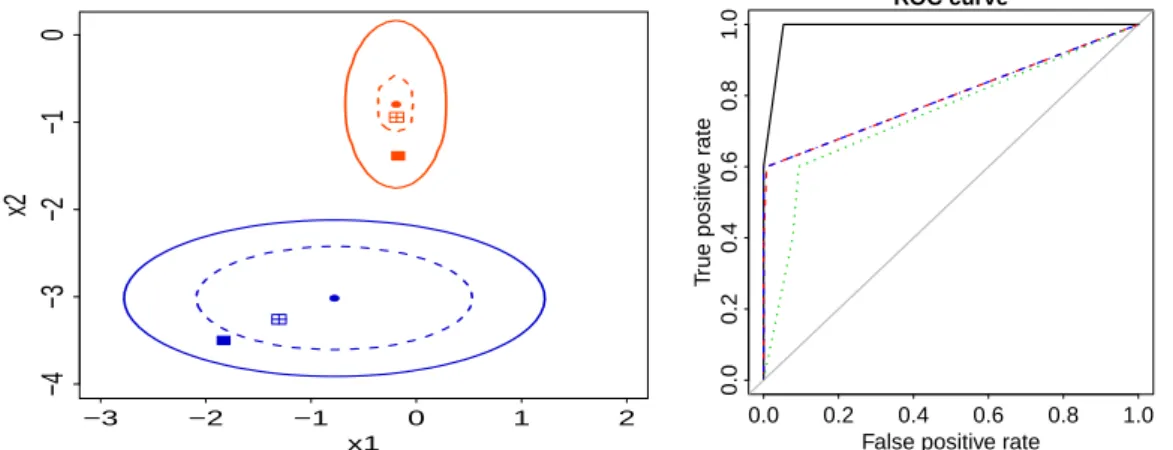
The generated data are illustrated in the right panel of Figure2. To better understand the rationale be-hindROSE, Figure3(left panel) shows two observations belonging to the prevalent and rare classes, and the surroundings within the observations are likely to be generated, for the two optionshmult.majo = 0.25,hmult.mino = 0.5.
Equipped with the new balanced samples generated byovun.sampleandROSE, we can train the classifiers and run them on the test set to assess their accuracy:
> tree.rose <- rpart(cls ~ ., data = data.rose) > tree.ov <- rpart(cls ~ ., data = data.bal.ov) > tree.un <- rpart(cls ~ ., data = data.bal.un) > tree.ou <- rpart(cls ~ ., data = data.bal.ou)
> pred.tree.rose <- predict(tree.rose, newdata = hacide.test) > pred.tree.ov <- predict(tree.ov, newdata = hacide.test) > pred.tree.un <- predict(tree.un, newdata = hacide.test) > pred.tree.ou <- predict(tree.un, newdata = hacide.test) > roc.curve(hacide.test$cls, pred.tree.rose[,2])
> roc.curve(hacide.test$cls, pred.tree.ov[,2], add.roc = TRUE, col = 2, lty = 2) Area under the curve (AUC): 0.798
> roc.curve(hacide.test$cls, pred.tree.un[,2], add.roc = TRUE, col = 3, lty = 3) Area under the curve (AUC): 0.749
> roc.curve(hacide.test$cls, pred.tree.ou[,2], add.roc = TRUE, col = 4, lty = 4) Area under the curve (AUC): 0.798
The returned AUCs clearly highlight the effectiveness of balancing the sample. An illustration of the ROC curves is given in the right panel of Figure3.
Adopting alternative estimators of accuracy
In real data applications, we often cannot benefit from the availability of additional data to test the accuracy of the estimated model (or if we can, we will probably use the additional information to train a more accurate model). Moreover, in imbalanced learning, the scarcity of data causes high variance estimates of the accuracy measure. Then, it is often appropriate to adopt some alternative methods to estimate model accuracy in place of the standard holdout. FunctionROSE.evalcomes to this aid by implementing a ROSE version of holdout, bootstrap or leave-K-out cross-validation estimators of the accuracy of a specified classifier, as measured according to a selected metric.
Suppose that a test set, to evaluate the accuracy of the classifier previously denoted astree.rose, is not available. We first exploitROSE.evalto obtain a ROSE-basedholdoutestimate of the AUC: > ROSE.holdout <- ROSE.eval(cls ~ ., data = hacide.train, learner = rpart,
method.assess = "holdout", extr.pred = function(obj)obj[,2], seed = 1) > ROSE.holdout
Holdout estimate of auc: 0.985
Similarly toROSE, the former instruction specifies the role of the columndatafrom which a ROSE sample is generated via argumentformula. The specification ofseedensures the generation of the same sample as the one used to buildtree.rose. Based on the synthetic sample, the classifier is built through an internal call to functionrpartspecified inlearner.
Argumentlearneris designed to recognize virtually all the R functions having a standard def-inition, as well as suitably user-defined functions, thereby allowing for a high flexibility in the employment of classifiers which exhibit non-homogeneous usage. As a consequence of such hetero-geneity, some caution is needed when specifying argumentlearner. In its simplest form,learneris a standard R function, that is, it has aformulaas a first compulsory argument and returns an object
x1
x2
● ● −3 −2 −1 0 1 2−4
−3
−2
−1
0
0.0 0.2 0.4 0.6 0.8 1.0 0.0 0.2 0.4 0.6 0.8 1.0 ROC curveFalse positive rate
T
rue positiv
e r
ate
Figure 3:Left panel: a zoomed view of two selected points of thehacide.traindata, the contour within which the ROSE artificial data are generated with probability 0.95 and an example of artificial points generated. The solid contour (and the associated filled points) refer to the use of the default smoothing parameters. The dashed contour (and associated points filled with a cross) refer to the use ofhmult.majo = 0.25andhmult.mino = 0.5. Right panel: ROC curves associated with classification trees built on data balanced according to different remedies. Solid line: data balanced by ROSE; dotted line: data balanced by undersampling; dashed (overlapping) lines: data balanced by oversampling and by a combination of over and undersampling.
whose class is associated with apredictmethod. As required by R conventions, the function name of the classifier and its R class should match. For example, in the chunk code above,learner = rpart is specified, as functionrpartreturns an object of classrpartto which apredict.rpartmethod is associated. Thus, functionpredict.rpartis internally called byROSE.evalto obtain a prediction. Also classifiers implemented by R functions with a non-standard usage can be passed tolearner. In this case,learnertakes a different form, as will be clarified subsequently in this section.
FunctionROSE.evalworks properly only when the prediction is a vector of class labels, prob-abilities, or scores from the estimatedlearner. Sincepredictmethods in R sources exhibit very non-homogeneous outputs, the optional argumentextr.predcan be deployed to pass a suitable user-defined function that filters relevant information from the output of any predict method and extracts a vector of predicted values. In the example above,predict.rpartreturns a matrix of predicted proba-bilities when fed with a classification tree. Hence, argumentextr.pred = function(obj)obj[,2]is defined as a function which extracts the column of probabilities of belonging to the positive class.
Along with the argumentlearner, functionROSE.evalrequires the specification of argument acc.measure, an accuracy measure to be selected amongc("auc","precision","recall","F"), which are the metrics supplied by the package. In the current example,acc.measurehas been left to its default value"auc", which determines an internal call to functionroc.curve. The other options entail an internal call to functionaccuracy.meas.
As an alternative to the ROSE-based holdout method, we may wish to obtain a ROSE version of the bootstrap accuracy distribution. By selectingmethod.assess = "BOOT", we fit the specified learneronBROSE samples and test each of them on the observed data specified in theformula. The optional argumenttraceshows the progress of model assessment by printing the number of completed iterations. The bootstrap distribution of the selected accuracy measure is then returned as output of functionROSE.eval.
> ROSE.boot <- ROSE.eval(cls ~ ., data = hacide.train, learner = rpart,
method.assess = "BOOT", B = 50, extr.pred = function(obj)obj[,2], seed = 1, trace = TRUE)
Iteration:
10, 20, 30, 40, 50 > summary(ROSE.boot) Call:
ROSE.eval(formula = cls ~ ., data = hacide.train, method.assess = "BOOT", B = 50, learner = rpart, extr.pred = function(obj) obj[, 2],
trace = TRUE, seed = 1)
Summary of bootstrap distribution of auc: Min. 1st Qu. Median Mean 3rd Qu. Max. 0.9282 0.9800 0.9839 0.9820 0.9860 0.9911
Similarly, we could obtain a leave-K-out cross validation estimate of the accuracy by selecting optionmethod.assess = "LKOCV". This option works as follows: the provided data, say of sizen, are split at random intoQ=n/Kgroups of size defined by argumentK; to speed up the computations, we setK = 5. However, in the presence of extreme imbalance between the classes, choosingKas low as possible is advisable, to not alter the class distribution in the data used for training. At each round, the specifiedlearneris estimated on a ROSE sample built on the provided data excluding one of these groups, and then a prediction on the excluded set of observations is made. At the end of the process, the predictions obtained on theQdistinct groups are deployed to compute the selected accuracy measure, which is then retrieved in the componentaccof the output ofROSE.eval. > ROSE.l5ocv <- ROSE.eval(cls ~ ., data = hacide.train, learner = rpart,
method.assess = "LKOCV", K= 5, extr.pred = function(obj)obj[,2], seed = 1, trace = TRUE)
Iteration:
10, 20, 30, 40, 50, 60, 70, 80, 90, 100,
110, 120, 130, 140, 150, 160, 170, 180, 190, 200 > ROSE.l5ocv
Call:
ROSE.eval(formula = cls ~ ., data = hacide.train, learner = rpart, extr.pred = function(obj)obj[, 2], method.assess = "LKOCV", K = 5, trace = TRUE, seed = 1)
Leave K out cross-validation estimate of auc: 0.973
In principle, the classification task would terminate here. However, one might wonder if different choices in the balancing mechanism or in the classifier estimation would lead to better results. To answer this question, we just need to set argumentscontrol.ROSEor, respectivelycontrol.learner accordingly. For example thehmult.majoand/orhmult.minoarguments could have been shrunk: > ROSE.holdout.h <- ROSE.eval(cls ~ ., data = hacide.train, learner = rpart,
extr.pred = function(obj)obj[,2], seed = 1,
control.rose = list(hmult.majo = 0.25, hmult.mino = 0.5)) or one could have grown a tree of a given complexity, in the following manner:
> ROSE.holdout.cp <- ROSE.eval(cls ~ ., data = hacide.train, learner = rpart, extr.pred = function(obj)obj[,2], seed = 1,
control.learner = list(control=list(cp = 0.05)))
Lastly, one could wish to compare the results with those obtained by using a different classifier. Suppose, for example, one is interested in fitting aK-nearest neighbors classifier. This is implemented, among others, by functionknnin packageclass. Functionknnhas a nonstandard R behaviour, both because it does not require aformulaargument and because model training and prediction are performed, by construction, simultaneously. The usage of functionknnis described by
knn(train, test, cl, k = 1, l = 0, prob = FALSE, use.all = TRUE)
wheretrainandtestare the training and the testing columns of predictors, respectively, andclis the vector of training class labels. To employknnas alearnerfunction inROSE.eval, we need to embed it within a suitable wrapper function which requires two mandatory arguments:dataandnewdata. The wrapper forknnis then:
knn.wrap <- function(data, newdata, ...){
knn(train = data[,-1], test = newdata, cl = data[,1], ...)}
where the first column is extracted as, in the currenthacideexample, it contains the class labels. Argumentsdataandnewdataare automatically filled when the wrapper is embedded inROSE.eval. Further arguments can be passed toknnthrough the usual argumentcontrol.learner, owing to the presence of argumentdotsin the wrapper. For example, we may specifyk=2 nearest neighbors and ask to return the predicted probabilities of belonging to the positive class as follows.
> rose.holdout.knn <- ROSE.eval(cls ~ ., data = hacide.train, learner = knn.wrap, control.learner = list(k = 2, prob = TRUE),
method.assess = "holdout", seed = 1)
As we can see, even if the employed classifier has a nonstandard implementation, it can be easily adapted to be used inside functionROSE.eval.
Bibliography
A. W. Bowman and A. Azzalini.Applied Smoothing Techniques for Data Analysis: Kernel Approach with S-Plus Illustrations. Oxford University Press, Oxford, 1997. [p80]
B. Efron and R. Tibshirani.An Introduction to the Bootstrap.Chapman and Hall, London, 1993. [p80] M. Kuhn. caret: Classification and Regression Training, 2014. URLhttp://CRAN.R-project.org/
package=caret. R package version 6.0-22. Contributions from Jed Wing and Steve Weston and Andre Williams and Chris Keefer and Allan Engelhardt and Tony Cooper and Zachary Mayer and the R Core Team. [p79]
N. Lunardon, G. Menardi, and N. Torelli. R packageROSE: Random Over-Sampling Examples (version 0.0-3). Università di Trieste and Università di Padova, Italia, 2013. URLhttp://cran.r-project.
org/web/packages/ROSE/index.html. [p79]
G. Menardi and N. Torelli. Training and assessing classification rules with imbalanced data. Data Mining and Knowledge Discovery, 28(1):92–122, 2014. [p79,80,81,85]
L. Torgo.Data Mining with R, Learning with Case Studies. Chapman and Hall/CRC, London, 2010. URL
Nicola Lunardon
Department of Economics, Business, Mathematics, and Statistics “Bruno de Finetti”, University of Trieste Piazzale Europa 1, 34100 Trieste, Italy
Giovanna Menardi
Department of Statistical Sciences, University of Padua via Cesare Battisti, 241, 35100 Padova, Italy
Nicola Torelli
Department of Economics, Business, Mathematics, and Statistics “Bruno de Finetti”, University of Trieste Piazzale Europa 1, 34100 Trieste, Italy