Computer Science Dissertations Department of Computer Science
Fall 12-18-2013
A Classification Framework for Imbalanced Data
Piyaphol Phoungphol
Follow this and additional works at:https://scholarworks.gsu.edu/cs_diss
This Dissertation is brought to you for free and open access by the Department of Computer Science at ScholarWorks @ Georgia State University. It has been accepted for inclusion in Computer Science Dissertations by an authorized administrator of ScholarWorks @ Georgia State University. For more information, please [email protected].
Recommended Citation
Phoungphol, Piyaphol, "A Classification Framework for Imbalanced Data." Dissertation, Georgia State University, 2013. https://scholarworks.gsu.edu/cs_diss/78
by
PIYAPHOL PHOUNGPHOL
Under the Direction of Dr. Yanqing Zhang
ABSTRACT
As information technology advances, the demands for developing a reliable and highly accurate predictive model from many domains are increasing. Traditional classification al-gorithms can be limited in their performance on highly imbalanced data sets. In this dis-sertation, we study two common problems when training data is imbalanced, and propose effective algorithms to solve them.
Firstly, we investigate the problem in building a multi-class classification model from imbalanced class distribution. We develop an effective technique to improve the performance
G-mean value. A ramp loss function is used to simplify and solve the problem. Experimental results on multiple real-world datasets confirm that our new method can effectively solve the multi-class classification problem when the datasets are highly imbalanced.
Secondly, we explore the problem in learning a global classification model from dis-tributed data sources with privacy constraints. In this problem, not only data sources have different class distributions but combining data into one central data is also prohibited. We propose a privacy-preserving framework for building a global SVM from distributed data sources. Our new framework avoid constructing a global kernel matrix by mapping non-linear inputs to a non-linear feature space and then solve a distributed non-linear SVM from these virtual points. Our method can solve both imbalance and privacy problems while achieving the same level of accuracy as regular SVM.
Finally, we extend our framework to handle high-dimensional data by utilizing Gener-alized Multiple Kernel Learning to select a sparse combination of features and kernels. This new model produces a smaller set of features, but yields much higher accuracy.
INDEX WORDS: Imbalanced Data, Privacy, Distributed Learning, Multiple Kernel Learning, Support Vector Machine, Feature Selection.
by
PIYAPHOL PHOUNGPHOL
A Dissertation Submitted in Partial Fulfillment of the Requirements for the Degree of
Doctor of Philosophy
in the College of Arts and Sciences Georgia State University
by
PIYAPHOL PHOUNGPHOL
Committee Chair: Professor Yanqing Zhang
Committee: Professor Raj Sunderraman Professor Robert Harrison Professor Yichuan Zhao
Electronic Version Approved:
Office of Graduate Studies College of Arts and Sciences Georgia State University December 2013
DEDICATION
To my beloved wife, Inthira, and my parents for their love, support, and encouragement over the years.
ACKNOWLEDGEMENTS
This dissertation work would not have been possible without the support of many people. First, I would like to thank my advisor, Dr. Yanqing Zhang for his help, guidance, encouragement on my research. A special thank you to Dr. Raj Sunderraman for generous help and advices throughout my time at Georgia State University. I also wish to thank my committee members, Dr. Harrison and Dr. Zhao, for taking time to review my work and give me creative comments to improve this dissertation.
I would like to acknowledge the continued financial support from the Computer Science Department, the Molecular Basis of Disease (MBD) fellowship, and the Second Century Initiative (2CI) fellowship at Georgia State University.
Last, I wish to express my gratitude to my parents and my wife for their understanding, continued support throughout all these years of my education.
TABLE OF CONTENTS ACKNOWLEDGEMENTS . . . v LIST OF TABLES . . . ix LIST OF FIGURES . . . x LIST OF ABBREVIATIONS . . . xi PART 1 INTRODUCTION . . . 1
1.1 Problem and Motivation . . . 1
1.1.1 Class Imbalance . . . 2
1.1.2 Multi-Source Imbalance . . . 5
1.2 Contributions . . . 6
1.3 Thesis Organizations . . . 7
PART 2 MULTI-CLASS CLASSIFICATION . . . 8
2.1 Sampling-based Approaches . . . 8 2.1.1 Under-sampling . . . 9 2.1.2 Over-sampling . . . 9 2.2 Feature Selection . . . 9 2.3 Cost-Sensitive Learning. . . 10 2.4 One-Class SVM. . . 11 2.5 Ensemble Methods . . . 12
PART 3 RAMP KERNEL MACHINE . . . 14
3.1 A New Objective Function . . . 14
3.2 Ramp Kernel Machine for Imbalanced Multi-class Data . . . 16
3.4 Solving Ramp Kernel Machines. . . 18
3.5 Evaluations . . . 19
3.5.1 Dataset . . . 19
3.5.2 Parameters & Performance Metrics . . . 20
3.5.3 Results . . . 21
3.5.4 Analysis of RKM Effectiveness . . . 25
PART 4 IMBALANCE DISTRIBUTED LEARNING . . . 27
4.1 Distributed Learning . . . 27
4.2 Possible Solutions . . . 28
4.2.1 Linear Regression . . . 29
4.2.2 Decision Tree . . . 30
4.2.3 Naive Bayes classifier . . . 31
4.3 SVM . . . 32
PART 5 SECURE SUM PROTOCOL . . . 35
5.1 Simple Secure Sum . . . 35
5.2 Secure Sum with Shamir’s Secret Sharing Scheme . . . 37
5.2.1 Homomorphic Encryption . . . 38
5.2.2 A Decentralized Voting Protocol . . . 38
5.3 Application of Shamir’s Secret Sharing to Distributed Data . . . 39
5.4 Privacy-Preserving K-means Over Distributed Data . . . 40
PART 6 PRIVACY-PRESERVING DISTRIBUTED SVM . . . 42
6.1 SVM . . . 42
6.1.1 SVM in Dual Form . . . 43
6.2 Kernel Approximation . . . 44
6.2.1 Selecting Landmarks . . . 44
6.3 Cutting Plane . . . 46
6.4 Evaluations . . . 49
6.4.1 Datasets . . . 51
6.4.2 Compared with Traditional Classification Models . . . 51
6.4.3 Compared with Other SVM-Based Approaches . . . 52
6.4.4 Efficiency . . . 54
PART 7 DISTRIBUTED FEATURE SELECTION . . . 58
7.1 Current feature selection . . . 58
7.1.1 Recursive Feature Elimination, SVM-RFE . . . 58
7.1.2 RELIEF . . . 60
7.2 Generalized Multiple Kernel . . . 60
7.2.1 Multiple Kernel Learning . . . 60
7.2.2 Generalized Multiple Kernel . . . 62
7.3 Feature Selection with Generalized Multiple Kernel . . . 63
7.4 GMKL over Distributed Privacy Framework . . . 64
7.4.1 GMKL in Primal Form . . . 64
7.4.2 Squared Hinge Loss (L2) Function . . . 65
7.5 Experiments . . . 66
7.6 UCI Datasets . . . 66
7.6.1 Performance Comparison . . . 67
PART 8 CONCLUSIONS & FUTURE WORK . . . 70
8.1 Conclusions . . . 70
8.2 Future Work . . . 71
8.2.1 Privacy-Preserving Distributed Multi-class SVM . . . 71
8.2.2 Semi-Supervised Learning . . . 72
LIST OF TABLES
Table 1.1 An example of data sources with different class distributions . . . 5
Table 3.1 Multi-class Imbalanced Datasets from UCI . . . 22
Table 3.2 Avg. G-mean Performance - Linear Kernel . . . 23
Table 3.3 Avg. G-mean Performance - RBF Kernel . . . 23
Table 3.4 Macro / Micro F-measure Performance . . . 24
Table 3.5 Contraceptive: class errors from Linear Cost-SVM model . . . 25
Table 3.6 Vertebral dataset class errors from Linear Cost-SVM model . . . . 25
Table 4.1 Horizontal Distributed Data . . . 27
Table 4.2 Vertical Distributed Data . . . 28
Table 6.1 Summary of datasets we used in the experiment. . . 51
Table 6.2 Performance comparison between Privacy Distributed SVM with tra-ditional classifiers. . . 52
Table 6.3 Performance of different algorithm based on different distributions 54 Table 6.4 Efficiency of Privacy Distributed SVM and SVM-ADMM onFour-class dataset. . . 55
Table 6.5 Efficiency of Privacy Distributed SVM and SVM-ADMM on Pima dataset. . . 55
Table 7.1 Performance Comparison of SVM, L2-SVM, and DGMKL. . . 67 Table 7.2 UCI results with datasets at different number of desired features,Nd. 68
LIST OF FIGURES
Figure 1.1 SVM on imbalanced dataset is biased toward the major class. . . 3
Figure 3.1 Composition of Ramp Loss . . . 17
Figure 3.2 An example of ConCave-Convex Procedure . . . 18
Figure 3.3 Contraceptive: Error distributions from Linear Cost-SVM . . . . 26
Figure 4.1 The structure of Cascade SVM . . . 32
Figure 4.2 Model synchronization in peer-to-peer network. . . 34
Figure 5.1 Secure computation of a sum. . . 36
Figure 5.2 An illustration of Adi Shamir concept. . . 37
Figure 5.3 An example of the Shamir’s Secret Sharing in voting protocol. . . 39
Figure 5.4 An application of Shamir’s Secret Sharing horizontal distributed data sources. . . 40
Figure 6.1 Components of privacy-preserving distributed SVM. . . 42
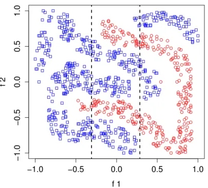
Figure 6.2 Four-class dataset is split into 3 groups by values of f1. . . 53
Figure 6.3 The number of iterations that ADMM uses in solving SVM for Four-class dataset. . . 56
Figure 6.4 The number of iterations that ADMM uses in solving SVM for Pima dataset. . . 57
LIST OF ABBREVIATIONS
• Acc - Accuracy
• Cost-SVM - Cost-Sensitive Multi-class Support Vector Machine • DGMKL - Distributed Generalized Multiple Kernel Learning • FP - False Positive
• FN - False Negative
• G-mean - Geometric mean
• GMKL - Generalized Multiple Kernel Learning • KNN - K-Nearest Neighbor
• MC-SVM - Multi-class Support Vector Machine • MKL - Multiple Kernel Learning
• PD-SVM Privacy-preserving Distributed Support Vector Machine • RBF - Radial Basis Function
• RKM - Ramp Kernel Machine
• ROC - Receiver Operating Characteristic • SVM - Support Vector Machine
• SVM-RFE - Support Vector Machine Recursive Feature Elimination • TP - True Positive
• TN - True Negative
PART 1
INTRODUCTION
1.1 Problem and Motivation
Recently, huge developments in science and technology have enabled the growth and availability of raw data to occur at an explosive rate. This has created an immerse oppor-tunity for knowledge discovery and data engineering research to play an essential role in a wide range of applications from daily life to national security, from enterprise information processing to governmental decision-making support systems, from micro-scale data analysis to macro-scale knowledge discovery. Techniques from data mining and machine learning are able to process structured data to extract meaningful patterns. Data mining algorithms learn by induction, so the data to be mined must be structured as a collection of examples of the target concept to be learned. Each example, or instance, is described by a set of attribute values, which typically are either numeric or categorical values.
From a set of structured examples of a target concept, a data mining algorithm can extract useful patterns, typically in one of three ways: clustering, association rule, and classification. Clustering and association rule mining are unsupervised learning processes, because they don’t involve the prediction of values for a specific attribute. Clustering involves partitioning the set of instances into groups such that examples in the same group are similar to each other based on some measure of similarity. Association rule mining involves looking for useful predictive patterns between any combinations of attributes in the data. This differs from supervised learning in that potentially interesting associations between any attributes or sets of attributes are sought. In supervised learning, one of the attributes, called the class attribute or dependent attribute, is meant to be predicted based on the values for the other attributes, called independent attributes. The process is called classification if the class attribute is categorical and regression or numeric prediction if the class attribute is
numeric. This work specifically addresses the problem of classification.
In classification, the objective is to successfully predict the values for the nominal class attribute (class label) of an example given the values for its independent attributes. Clas-sically, success in this endeavor is measure by overall accuracy, the percentage of instances for which the class label is correctly predicted. Classification algorithms, of which there are many, were often designed in the spirit of achieving the maximum possible number of correct class label predictions. In order to extrapolate reliable patterns from a dataset so that future instances can be classified accurately, the information contained in the data must be valid. Unfortunately, in real world classification applications, data is rarely perfect. A number of issues can affect the quality of the data used to train a classifier, often leading to reduced classification accuracy
1.1.1 Class Imbalance
In many real-world classification applications, such as software prediction, oil spill de-tection from satellite images, dede-tection of fraudulent online credit card, diagnosis of rare diseases, training data might be imbalance [1–3] where the number of data in some classes are extremely smaller than other classes. This is usually caused by the rarity of cases/events or by limitations on data collection process such as high cost or privacy problems. For ex-ample, biomedical data that derived from a rare disease and an abnormal condition, or some data that often obtained via expensive experiments.
The fundamental issue with the imbalanced learning problem is the ability of imbalanced data to significantly compromise the performance of most standard learning algorithms. Most algorithms usually assume balanced class distributions or equal misclassification costs. This problem will cause most standard machine learning algorithms to be biased toward the majority class because they try to optimize overall accuracy, which is overwhelmed by ma-jority classes and ignore minority class. Therefore, when presented with complex imbalanced data sets, these algorithms fail to properly represent the distributive characteristics of the data and result in unfavorable accuracies across the classes of the data.
/ĚĞĂů>ŝŶĞ
^sD
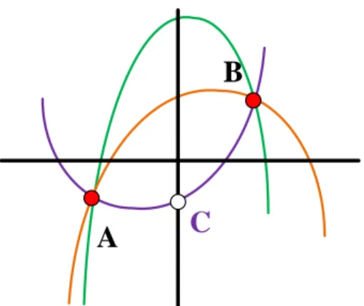
Figure (1.1) SVM on imbalanced dataset is biased toward the major class.
This problem has posed a significant drawback of the performance achieved by existing classification system. In the biomedical field, this issue is particularly crucial since learn-ing from these imbalanced data can help us discover useful knowledge to make important decisions while it can also be extremely costly to misclassify these data.
An example of biased classifier between two imbalanced classes (RED & BLUE marks) is shown in Fig. 1.1. SVM gives an biased separate line because it tries to minimize the total of classification errors which is dominated by errors of the major class instances(RED). Therefore, the SVM line is shifted away from the major class (RED) toward the minor class (BLUE).
Data Noise Noisy data which often occurs with class imbalance data is another
com-mon data quality issue that tends to impair classification performance. Data noise occurs when dependent attribute values are recorded erroneously. Unfortunately, most traditional classifiers cannot handle noisy data efficiently and its classification accuracy depends vitally on the quality of the training data. A few noisy data can seriously deteriorate the classifier’s performance. Because most classifier try to minimize the total classification errors, but an error of each data point can vary from 0 to +∞, therefore errors of a few bad or noisy points can dominate or compromise the overall errors which result in classifier’s performance dete-rioration. Accordingly, one way to improve the overall classification accuracy is to eliminate the noise or bad data points from the training data.
Multi-class Class Imbalance In the typical binary class imbalance problem, one class vastly outnumbers the other. However, real-world problems often require classification between more than two classes. The multi-class classification problem is an extension of the traditional binary class problem where a data set consists k classes instead of two. While imbalance is said to exist in the binary class imbalance problem when one class severely outnumbers the other class, extended to multiple classes the effects of imbalance are even more problematic. That is, given k classes, there are multiple ways for class imbalance to manifest itself in the data set. One typical way is there is one ”super majority” class which contains most of the instances in the data set. Another typical example of class imbalance in multi-class data sets is the result of a single minority class. In such instances k−1 instances each make up roughly 1/(k − 1) of the data set, and the ”minority” class makes up the rest. The multi-class imbalance problem is therefore interesting for two important reasons. First, most learning algorithms do not deal with the wide variety of challenges multi-class imbalance presents. Secondly, a number of classifiers do not easily extend to the multi-class domain.
There are many research works that try to improve traditional techniques or develop new algorithms to solve the class imbalance problem. However, most of those studies are focused only on binary case or two classes and solutions for binary class problems are not applicable directly to class cases. One common solution is to decompose the multi-class problems into a set of binary multi-class problems, i.e., multi-classifying each individual multi-class versus all the other classes. This enables users to learn binary class classifiers on each of the sub problems which can then be combined into an ensemble in order to solve the multi-class problem. However, the obvious drawbacks of this solution are: 1) to learn an identification model for each class is expensive in training; 2) results of each class label assignment are not comparable due to the decision can be made differently for different classes; and 3) one class versus the other classes will worse the imbalanced distribution even more for the small classes.
Table (1.1) An example of data sources with different class distributions Source Proportion of class A Proportion of class B
S1 15% 85%
S2 80% 20%
S3 50% 50%
1.1.2 Multi-Source Imbalance
Recent advances in computing, technologies, storage methods, and scientific research have resulted in many large scale and decentralized environments in which both data and computation are distributed through several sources instead of being collected in a single source. This has drawn a significant amount of interest from both academic and industry. comparing patterns from different databases and understanding their relationships can be extremely beneficial for applications such as bioinformatics, health informatics sensor net-working, and business intelligence. In particular, important information such as pattern trends and knowledge of decision rules buried in each individual database are very hard to be discovered by only examining a single data set, whereas comparatively mining multiple databases will enable users to discover interesting patterns across a set of data collections that would not have been possible otherwise.
Although these data collected through multiple sources need to be used for classification in order to achieve higher classification accuracy and robustness, unfortunately, they are heterogeneous and have different distributions and underlying patterns among data sources. One possible solution is to combine data from multiple sources together into a single location. However, in real world application, data can often only be accessed from local database but cannot be easily merged to any other databases directly due to many reasons such as client privacy, large data sizes, power consumption limit, and different geographical locations of data sources. Therefore, learning correlating information from multiple data sources has become a crucial and challenging problem in data mining and knowledge discovery.
random forests have been proposed for integration a predicting model from multiple sources. However, none of these work considers or pays attention to the class distribution differences among data sources. These differences do not have much effect on the performance of the combined model if all data sources have the same or closely similar class distributions. On the other hand, if data sources have extremely different class distributions, it can degrade the performance of integration model. For example, if we try to create a combined learning model from three data sources S1, S2, S3 to distinguish data in class A from class B. The
class distributions of each data source are shown in Table 1.1. It can clearly be seen that the predicting model from S1 and S2 will be biased; S1 is leaning towards class A while
S2 is leaning towards class B. As a result, the combined model from S1, S2, and S3 using
traditional ensemble techniques will have a poor performance.
1.2 Contributions
Multi-class Imbalance Classification Model First, we re-formulate multi-class
SVM to optimize G-mean, which is one of most popular measure for multi-class imbalance classification. We simply the proposed optimization problem with Ramp Loss function, and then find an efficient method to solve it. In the experiments, our model provides much more accurate results than traditional models.
Privacy-Preserving Distributed Classification Model Second, we present a
so-lution framework that overcomes the privacy constraint in constructing SVM from dis-tributed data. Moreover, the proposed framework can handle the class imbalance among data sources, and yields a comparable classification result to a standard model that trained by combining all data in a single location.
Privacy-Preserving Distributed Feature Selection Last, we extend our
privacy-preserving distributed SVM model to handle high-dimensional data. The extended frame-work applied Generalized Multiple Kernel Learning (GMKL) to select a sparse combination
of features and their kernel parameters. The final result proved that the new framework can maintain or even improve accuracy of the original model while using a much smaller set of features.
1.3 Thesis Organizations
The rest of this dissertation is organized as follows.
Chapter 2: Multi-class Classification We provide an extensive literature review
on applying binary classification tools to multi-class problem, and many popular methods to solve this imbalanced multi-class problem. We also cover several effective metrics for evaluating classification model on imbalanced data.
Chapter 3: Ramp Kernel Machines The detail of our Ramp Kernel Machines and
technique used to solve its optimization problem are presented in this chapter. Experiment results on 10 real-world datasets to compare its performance with other solutions are also discussed.
Chapter 4-5: Multiple Sources Learning We explore the current possible
so-lutions for the imbalance problem in multi-source learning. Furthermore, we describe the secure sum protocol and its application on K-means clustering.
Chapter 6: Privacy-Preserving Distributed SVM We describe components and
techniques we use to build SVM from distributed data while still protecting data privacy.
Chapter 7: Distributed Feature Selection We explain details and problems in
applying GMKL to our distributed SVM framework in order to select features from high-dimensional data.
Chapter 8: Conclusion & Future Work We summarize and discuss the possible
PART 2
MULTI-CLASS CLASSIFICATION
In recent years, many researchers have studied the problem of imbalanced data classifi-cation and tried to improve the performance of classificlassifi-cation models. However, most of their work is concentrated on binary classification problem. Only few studies have been extended to multi-class scenario, which is more realistic and can be generalized ton-class classification problem.
Adopting techniques that showed successful results for binary case to multi-class scenario is not quite easy and straightforward. Some general ideas at data level such as feature selection [4], sampling-based approach can easily apply to multi-class problem directly, while it is difficult for many algorithm-specific techniques [5, 6]. We have grouped the related work that shows promising results in improving multi-class imbalance classification into the following categories.
2.1 Sampling-based Approaches
Sampling is a simplest strategy in dealing with class imbalance problem; by changing original class frequencies at a preprocessing step to balance the class distribution of training data. Thus, this approach requires no change to an original learning algorithm at all. It could involve under-sampling, over-sampling, or both. The amount to sample in each class can be chosen empirically [1] or in relation to its misclassification cost [7, 8]. The concern is that under-sampling might remove some potentially valuable information, while over-sampling could also lead to over-fitting. Therefore, many algorithms combine under-sampling and over-sampling to gain advantages from both.
2.1.1 Under-sampling
Under-sampling changes the training sets by sampling a subset of major class and repeating minor class instances. In order to avoid losing any useful information contained in the ignored examples, clustering techniques are used in selecting a subset of training data [9]. Liu [10] suggested a technique that is similar to the balanced Random Forest [11] called
EasyEnsemble by generatingT balanced sub-problems. Then, the outputs of sub-problems are combined together with AdaBoost.
2.1.2 Over-sampling
Over-sampling increases the number of the minority class instances by duplicating the instances of the minority. Chawla [12], introduced a more complicated technique called
SM OT E which generates a synthetic examples rather than over-sampling with replacement. The synthetic examples are created by joining any/all the line segments of the k minority class nearest neighbors.
However, few experiments on sampling-based approach have been carried out with and designed for multi-class cases. According to [8], sampling methods are only useful for binary imbalance problems. They are not effective in dealing with multi-class imbalance prob-lems and could even degrade classifiers performances when the number of classes is high or imbalance is severe.
2.2 Feature Selection
The goal of feature selection in general is to select a subset of features that allows a classifier to reach optimal performance. Feature selection is a key step for many machine learning algorithms especially when the data is high dimensional such as microarray-based classification data sets which often have tens of thousands of features, and text classification data sets using just a bag of words feature set have orders of magnitude more features than documents [13]. A number of researchers have conducted research on using feature selection
to combat the class imbalance problem [13] [14].
Feature selection metrics are commonly used to rank features independent of their con-text with other features. It shows how effective of each individual feature in predicting the class of each sample. Wasikowski developed a new feature selection metric, F AST [15], specifically designed to handle small sample imbalanced data sets. F AST is based on the area under the receiver operating characteristic (AUC) generated by moving the decision boundary of a single feature classifier with thresholds placed using an even-bin distribution. Cao [16] applied the stochastic algorithm Optimal F eature W eighting (OFW) and one-vs-one SVM in searching for optimized features (the gene predictors) from imbalanced and high-dimensional feature space of microarray data.
2.3 Cost-Sensitive Learning
In cost-sensitive learning, it considers the costs of misclassification data in one class to another class, and then try to minimize total costs rather than total errors. A widely used approach in applying cost-sensitive approach to SVM [17], is to assign a higher penalty error for a minority class in the optimization problem.
To facilitate this approach, Zhou & Liu recommended a rescaling technique [8] in con-verting a confusion matrix ij to class penalty factors for multi-class SVM model. The
weights of each classeswr will be rescaled simultaneously according to their misclassification
costs. Solving the relations in (2.1) will get relative optimal weights of imbalanced data. Then, multi-class SVM will be trained using these optimized weight.
w1 w2 = 1,2 2,1, w1 w3 = 1,3 3,1, . . . , w1 wm = 1,m m,1 w2 w3 = 2,3 3,2, . . . , w2 wm = 2,m m,2 . . . , . . . . . . , wm−1 wm = m−1,m m,m−1 (2.1)
In the case that a confusion matrix or misclassification costs are unknown, Sun [18] applied Genetic Algorithm to search for optimized values, and then evaluate them with
multi-class AdaBoost algorithm, AdaBoost.M1 [19]. In each iteration, the algorithm will update the weight of its base learners based on their class predictions and misclassification cost of an incoming data. However, Sun’s approach is computational expensive and practical only when a number of class is small. Landgrebe [20] suggested a pairwise analysis which investigates the interactions between each pair of classes, instead of random searching. The pairwise approach optimizes misclassification costs by a greedy-search that maximizes an approximate multi-class ROC and ignores neglectable interactions, resulting in a fast and scalable algorithm.
2.4 One-Class SVM
Unlike standard SVM, one-class SVM only recognizes examples from one class rather than differentiating all examples. It is useful when examples from the target classes are rare or difficult to obtain. One-class SVM [21] maps data into feature space and then try to use a hypersphere (ball) to describe data by putting most of the data into the hypersphere. This can be formulated into an optimization problem in (2.2) where the ball should be as small as possible, at the same time, include positive training data as much as possible. The classification is based on the predetermined threshold,ν ∈[0,1], which indicates whether to include the instance to the target class or not. When ν is small, more data will be put into the ball. On the other hand, when ν is larger, the size of the ball will be squeezed.
min R R 2 + 1 n ν n X i=1 ξi s.t. ∀i | φ(xi)−c|2 ≥ R2 + ξi ; ξi ≥ 0 (2.2)
Raskutti [22] demonstrated the optimality of one-class SVMs over two-class ones in certain important imbalanced-data domains, including genomic data. In particular, they showed that one-class learning is particularly useful when used on extremely unbalanced data sets composed of a high dimensional noisy feature space.
In order to apply one-class SVM to multi-class problem, multiple models of one-class SVM will be trained together. Hao & Lin [23] formulated multiple one-class SVM models as one large optimization problem to minimize the total errors, while [24, 25] used multiple one-class SVM models with One-vs-One strategy and iteratively adjusted the threshold of each models to maximize the total accuracy.
The main challenging problem is selecting proper thresholds for each class: setting a high threshold value would make an inclusion more difficult, so positive examples are more likely to be misclassified. Yet, setting the value too low would allow more examples from non-target classes in the target class region.
2.5 Ensemble Methods
Ensemble methods intelligently combine the predictions of a number of classifiers and make one prediction for a sample based on multiple classifiers. For imbalanced datasets, where any single classifier is likely not to generalize well to the data, it is possible to achieve substantial improvements in performance by using many individual classifiers together. The individual classifiers in an ensemble are trained using randomly selected subsets of the full data set. As long as each subset is sufficiently different from the others, each classifier will realize a different model, and an ensemble may give a better overall view of the learning task. Research on ensemble methods has mainly focused on two different techniques: bagging and boosting.
Bagging was initially developed by Breiman [26]. In a bagging ensemble, each individual classifier is trained using a different bootstrap of the data set. A bootstrap from a data set of N samples is a randomly drawn subset of N samples with replacement. The replacement allows samples to be drawn repeatedly. The most popular bagging ensemble is the random forest [27]. The random forest uses decision trees as the individual classifier. Before train-ing the individual decision trees on their bootstraps, a random feature selection algorithm removes all but a small number of the features to increase the speed of training and the disparity between models. Because the random forest tries to maximize the accuracy of its
predictions, it suffers from the class imbalance problem.
Boosting was introduced by Schapire [28] as a way to train a series of classifiers on the most difficult samples to predict. The first classifier in a boosting scheme is trained using a bootstrap of the data. Then, test that classifier on the whole data set and determine which samples were correctly predicted and which were incorrectly predicted. Boosting Classifier iteratively improves the classifiers’ performance for imbalanced data sets by either updating misclassification cost [29] or changing the distribution ratio [6, 30] of each class. Some recent studies [18, 31] extended this approach to multi-class imbalance problem and achieved promising results.
PART 3
RAMP KERNEL MACHINE
In this chapter, we will explain details of our proposed solution, Ramp Kernel Machine (RKM), to solve the multi-class imbalanced classification problem. Our algorithm is based on Crammer & Singer multi-class formulation [32] discussed in Part 2. However, in our case, we did not try to optimize the total classification error because the total error or accuracy tends to be dominated by the major class or bad data points when a training data is noisy and imbalanced. Thus, we modified the objective function to maximize a metric that is more effective for imbalanced data than the total accuracy.
3.1 A New Objective Function
Among popular matrices used for imbalanced classification, we decided to choose the geometric mean or G-mean as a part of our objective function because it is one of the most popular measures and easier to calculate than F-measure and multi-class AU C. Thus, in classifying m class problem from n training samples x1, x2, ..., xn where xi is a point in
feature space Rd with labely
1, y2, ..., yn ∈ {1, . . . , m}, The new optimization problem which
maximizes margin between classes and G-mean can be re-defined as (3.1) where W is a
m×dmatrix andWr, the rth row ofW, is a coefficient vector of classr,C is a regularization
parameter and ξi is an error in predicting point i.
max W C m Y r=1 m p Accr− 1 2kWk 2 (3.1) s.t.∀i,∀r6=yi, Wyi·xi−Wr·xi+ξi ≥ 1 ∀i, ξi ≥ 0
The predicted label of test datax is a class having the highest similarity score which can be calculate from (3.2) where Wr, the rth row ofW, is a coefficient vector of class r.
f(x) = arg max
r∈Y
Wr·x (3.2)
Asm is constant, the objective function in (3.1) can be rewritten as a minimization problem as (3.3) min W 1 2kWk 2− C0 m Y r=1 Accr (3.3)
The objective function in (3.3) should yield the best perfect model for multi-class im-balanced classification as it is directly derived from G-mean. However, in practice, it is quite computational expensive to find a solution of the optimized problem when the objective function is not continuous, non-linear, and non-convex function. Only few methods such as a genetic algorithm [33], a particle swarm optimization [34] are able to solve this problem.
In order to make the problem easier to solve, we decide to modify the objective in (3.3) by using an average of all accuracies instead of a geometric mean of all accuracies in G-mean. The modified objective function will be reformulated as:
min W 1 2kWk 2− C m m X r=1 Accr (3.4)
Let`be 0-1 loss function;`i is equal to 0 when a predicting label ofiis correct, and equal to 1
when a predicting label ofiis invalid. Thus, the accuracy of classr,Accr =
Pn
i|yi=r(1−`i)/Nr whereNris the total number of data in classr. If we defineδi,r as a 0-1 membership function
class r will be Accr =Pni=1δi,r(1−`i)/Nr. We can rewrite (3.4) as (3.5) . min W 1 2kWk 2 − C m m X r=1 n X i=1 δi,r(1−`i) Nr ≈ min W 1 2kWk 2 + n X i=1 (C 0 Nyi ) `i ≈ min W 1 2kWk 2 + n X i=1 Cyi`i (3.5)
We can notice from (3.5) that the new objective is very close to the standard objective function, but the main differences are 1.) a regularization parameter of each point is weighted inversely by the number of data in the same class, C0/Nyi That is similar to a concept in cost sensitive learning. 2.) an error/loss of each point `i is 0-1 or step function. Although
the problem (3.5) is less complex than (3.3) and can be solved as Mixed Integer Quadratic Programming (MIQP) by popular solvers, the solving process is still very computationally-expensive. In the next section, we will find an alternative way to simplify (3.5) and solve it efficiently.
3.2 Ramp Kernel Machine for Imbalanced Multi-class Data
Many studies tried to solve SVM with 0-1 loss function by replacing it with other smooth functions such as sigmoid function [35] [36], logistic function [37], polynomial function [36] , and hyperbolic tangent function [38]. These functions, while yielding accurate result, still suffer from being computationally-expensive when solved as an optimization problem due to its non-convex nature. Alternatively, a truncated hinge loss or ramp loss function which is a non-smooth but continuous function has been proved to be accurate and efficient for SVM problem [39–41]. Due to its efficiency and simplicity, we decide to use the ramp loss to simulate 0-1 loss function in (3.5).
The ramp loss or truncated hinge loss will be in range [0,1] when error ξ is less than a constant ramp parameter, z and will be equal to 1 when ξ is greater thanz. An example of ramp loss function is shown in Fig 3.1(a). It is obvious that the ramp loss: R(ξ) is equal to
ʇ Z;ʇͿ
ϭ
nj (a) Ramp Loss
ʇ ,;ʇͿ ϭ nj (b) Hinge Loss ʇ ,nj;ʇͿ ϭ nj (c) Hz: max(0, ξ−z)
Figure (3.1) Composition of Ramp Loss
the original hinge loss: ξ in Fig 3.1(b) minus a truncated part: Hz in Fig 3.1(c).
R(ξ) =ξ−Hz(ξ) (3.6)
When we replace `i in (3.5) withR(ξi), the objective function will be:
min W 1 2kWk 2 + n X i=1 Cyiξi− n X i=1 CyiHz(ξi) (3.7)
Although the objective function in (3.7) is non-convex, Karush-Kuhn-Tucker conditions re-main necessary (but not sufficient) optimality conditions. In the next section, we will intro-duce an efficient method to solve it.
3.3 ConCave-Convex Procedure (CCCP)
Due to the non-convex nature of objective function in (3.7), solving this problem is not easy and straightforward as normal convex optimization problem. We used the popular algorithm called ConCave-Convex Procedure (CCCP) [42] to solve our non-convex objective function. CCCP was first introduced by Yuille & Rangarajan to solve any non-convex opti-mized problems. According to CCCP, any objective functions, f(x) can be decomposed into the sum of a convex function and a concave function: f(x) = fvex(x) +fcave(x). CCCP will
Figure (3.2) An example of ConCave-Convex Procedure
solve non-convex optimized problem iteratively by approximating the concave part from its tangent ∂fcave/∂x and a current solution of convex function,xt, until a result is convergent.
fcavet (x) = ∂fcave ∂x ·x t xt+1 = arg min x fvex(x) +fcavet (x) (3.8)
A graphical illustration of CCCP is showed in Fig 3.2. Assumed that we want to minimize the function in Fig 3.2 (left): E(~x). We first decompose it into Fig 3.2 (right): a convex part (top curve) E1(~x) minus a convex term (bottom curve) E2(~x).The algorithm
proceeds by matching points on the two terms which have the same tangents. For an input
x0, we calculate the gradient ∇E2(x~0) and find the point x1 such that ∇E1(x~1) =∇E2(x~0)
Next, we determine the point x2 such that ∇E1(x~2) = ∇E2(x~1), and repeat. Finally, the
algorithm rapidly converges to the solution at ~x= 5.0.
3.4 Solving Ramp Kernel Machines
In order to apply CCCP to our objective functions (3.7), we first decompose the objective function into convex and concave parts in (3.9).
min W 1 2kWk 2 + n X i=1 Cyiξi | {z } convex − n X i=1 CyiHS(ξi) | {z } concave (3.9)
The tangent of concave parts will be:
∂ft cave ξi = 0 if ξt i ≤z −Cyi if ξ t i > z (3.10)
Thus, in each iteration, CCCP will solve the optimized problem in the form of:
min W 1 2kWk 2 + n X i | ξt i≤z Cyiξi (3.11) s.t.∀i,∀r6=yi, Wyi·xi−Wr·xi+ξi ≥ 1 ∀i, ξi ≥ 0
The problem (3.11) can easily be reformulated into dual form using the same technique used by Crammer & Singer [32]. Therefore, the complete step in solving Ramp Kernel Machine is shown in Alg 1. Points having one or more of non-zeroαi,r will besupport vector
points of the model.
Interestingly, the Ramp Kernel Machine in Alg. 1 looks complex and requires to solve an optimization problem multiple times until its solution is converged. In fact, the successive optimizations only refine existing support vectors from the previous iteration. Therefore, it will be much faster because their solutions have roughly the same group of support vectors.
3.5 Evaluations
3.5.1 Dataset
In order to evaluate the performance of our proposed solution, Ramp Kernel Machine (RKM), we have compared it against other popular multi-class SVM classifiers; Crammer
Algorithm 1 Ramp Kernel Machine
1: find ratios of each class: ratior
2: calculate Cr for each class:
Cr =C/ratior 3: initialize α 4: repeat 5: compute ξi = 1+ maxm r6=yi Pn j=1αj,rK(xi, xj)− Pn i=1αj,yiK(xi, xj) 6: minα 12Pni=1Pni=1K(xi, xj)−Pni=1 αi,yi s.t. αi,r ≤ Cyi if r=yi and ξi ≤z 0 otherwise 7: until α converges 8: f(x) = arg maxr∈Y Pn i=1αi,rK(xi, x)
& Singer multi-class SVM (MC-SVM) [32] and cost-sensitive multi-class SVM (Cost-SVM). The experiments use 10 real-world imbalanced datasets from multiple domains including Thyroid Disease, Yeast, Contraceptive Method, Vertebral Column, Heart Disease, and Pima Diabetes datasets. These datasets are publicly available from the UCI repository [43] and their characteristics are summarized in Table 3.1. The binary-class Pima Diabetes dataset is selected to show that our ramp kernel machine is a general n-class classifier which is applicable to 2-class problem as well. For each dataset, we calculated class ratios, and then marked its smallest rmin and largest rmax class ratios by asterisk (?). The imbalance of the
datasets are indicated by the high ratio between the number of instances of the majority class and the minority class; rmax/rmin.
3.5.2 Parameters & Performance Metrics
In the experiments, we implemented all three algorithms in Java and used Gurobi Op-timizer [44] to solve the optimization problems. We experimented with two types of kernels: linear and non-linear (Radial Basis Function, RBF) kernels. Parameters: cost (C), and RBF Gamma (γ) of each algorithm are tuned using grid search with 5-fold cross validation
to maximize G-mean where C ∈[2−2,2−1, . . . ,215],γ ∈[2−6,2−5, . . . ,25]. Then, Ramp-cut
(z) parameter of RKM is selected by grid search over a range [0.1,0.2, . . . ,2.0] while keeping the values of C and γ parameters the same as in Cost-SVM algorithm.
For each dataset, we ran 40 trials; in each trial, eighty percent of data are randomly selected as training data while the rest are used as test data. Then, a G-mean value of a model is calculated from the accuracies of each class. The average G-mean for linear and RBF kernels are shown in Table 3.2 and Table 3.3 respectively. In addition to G-mean, we investigated the micro and macro-averaging F-measure of the model in Table 3.4.
3.5.3 Results
Table 3.2 and Table 3.4 clearly show that in linear kernel, the ramp kernel machine yields better classification results than cost-sensitive model and original multi-class SVM, with respect to both G-mean and F-measure. Indeed, the performance improvements of RKM are significant when comparing with MC-SVM & Cost-SVM on datasets with low average G-mean value such as Yeast, Contraceptive Method, Heart Disease; despite the fact that those datasets have very high imbalance ratio (Yeast = 92.60, Heart Disease-Switzerland = 9.60, Heart Disease-Cleveland = 12.62).
In the RBF kernel, the ramp kernel machine generally achieves the best performance among three algorithms; it has the highest G-mean and F-measure in all datasets except the lower F-measure in Yeast and Heart Disease (Switzerland) datasets. Nevertheless, it is relevant to point out that parameters used in the experiments are selected to maximize G-mean value, not F-measure. The improvements of RKM are less significant than linear kernel case, possibly due to the higher-dimensional feature space and non-linear nature of RBF kernel.
22
Datasets # Instances # Attributes # Classes Class Ratios, r Imbalance Ratio
rmax/rmin Thyroid Disease 3772 21 3 0.025?, 0.050, 0.925? 37.51 Yeast 1484 8 10 0.312?, 0.289, 0.164, 0.110, 0.034 92.60 0.030, 0.024, 0.020, 0.014, 0.003? Contraceptive Method 1473 9 3 0.427?, 0.226?, 0.347 1.89 Vertebral Column 310 5 3 0.193?, 0.484?, 0.323 2.50
Heart Disease (Switzerland) 123 13 5 0.076, 0.381?, 0.276, 0.219, 0.048? 9.60
Heart Disease (Cleveland) 303 13 5 0.541?, 0.182, 0.119, 0.115, 0.043? 12.62
Pima Diabetes 768 8 2 0.651?, 0.349? 1.87
Glass Indentification 214 9 6 0.327, 0.079, 0.355?, 0.061, 0.136, 0.042? 8.44
Page Blocks 5473 10 5 0.898?, 0.060, 0.005?, 0.016, 0.021 175.46
Wine Quality (Red) 1599 10 6 0.006?, 0.033, 0.426?, 0.399, 0.125, 0.011 68.1
23 Datasets MC-SVM Cost-SVM RKM Thyroid Disease 0.945 0.991 0.996 Yeast 0.382 0.513 0.576 Contraceptive Method 0.303 0.327 0.513 Vertebral Column 0.776 0.835 0.847
Heart Disease (Switzerland) 0.304 0.553 0.586
Heart Disease (Cleveland) 0.367 0.454 0.481
Pima Diabetes 0.492 0.703 0.735
Glass Indentification 0.782 0.789 0.848
Page Blocks 0.924 0.978 0.982
Wine Quality (Red) 0.509 0.520 0.659
∗
the bold number means RKM has better performance than the other two classifiers.
Table (3.3) Avg. G-mean Performance - RBF Kernel
Datasets MC-SVM Cost-SVM RKM
Thyroid Disease 0.961 0.968 0.986
Yeast 0.908 0.912 0.937
Contraceptive Method 0.735 0.743 0.786
Vertebral Column 0.931 0.933 0.967
Heart Disease (Switzerland) 0.897 0.912 0.920
Heart Disease (Cleveland) 0.899 0.905 0.932
Pima Diabetes 0.913 0.938 0.951
Glass Indentification 0.926 0.934 0.979
Page Blocks 0.933 0.951 0.966
Wine Quality (Red) 0.805 0.898 0.930
24
Datasets Linear Kernel RBF Kernel
MC-SVM Cost-SVM RKM MC-SVM Cost-SVM RKM
Thyroid Disease 0.886 / 0.903 0.923 / 0.930 0.943 / 0.949 0.970 / 0.974 0.971 / 0.975 0.993 / 0.994
Yeast 0.465 / 0.476 0.507 / 0.541 0.531 / 0.572 0.963 / 0.967 0.969 / 0.972 0.964 / 0.969 Contraceptive Method 0.369 / 0.417 0.380 / 0.464 0.402 / 0.493 0.761 / 0.766 0.772 / 0.778 0.811 / 0.819
Vertebral Column 0.786 / 0.801 0.813 / 0.825 0.814 / 0.827 0.960 / 0.962 0.977 / 0.980 0.983 / 0.984
Heart Disease (Switzerland) 0.685 / 0.706 0.673 / 0.724 0.721 / 0.768 0.948 / 0.956 0.984 / 0.987 0.961 / 0.969 Heart Disease (Cleveland) 0.587 / 0.672 0.616 / 0.690 0.642 / 0.694 0.954 / 0.959 0.965 / 0.971 0.973 / 0.978
Pima Diabetes 0.577 / 0.605 0.671 / 0.686 0.679 / 0.694 0.956 / 0.958 0.972 / 0.972 0.975 / 0.975
Glass Indentification 0.666 / 0.672 0.794 / 0.823 0.841 / 0.861 0.934 / 0.936 0.964 / 0.966 0.989 / 0.992
Page Blocks 0.735 / 0.738 0.776 / 0.804 0.843 / 0.871 0.895 / 0.897 0.967 / 0.971 0.990 / 0.991
Wine Quality (Red) 0.246 / 0.248 0.298 / 0.404 0.439 / 0.527 0.550 / 0.557 0.907 / 0.912 0.930 / 0.934 1 the first number is macro-averaging F-measure and the second number is micro-averaging F-measure.
Table (3.5) Contraceptive: class errors from Linear Cost-SVM model Classes Average of Scaled Error Variance of Scaled Error
No-use 1.24 3.20
Long-term 16.99 48.62
Short-term 5.74 18.38
Table (3.6) Vertebral dataset class errors from Linear Cost-SVM model Classes Average of Scaled Error Variance of Scaled Error
Disk Hernia 1.38 1.84
Spondylolisthesis 1.00 1.12
Normal 1.53 1.02
3.5.4 Analysis of RKM Effectiveness
We have studied the effectiveness of using ramp-loss in imbalanced data classification. Why does the ramp kernel machine yields much better result than the cost-sensitive multi-class SVM on some datasets, such as Contraceptive, and Yeast, but shows only slight effects on some datasets such as Vertebral Column, and Thyroid Disease ? We provided more de-tailed analysis by examining the distributions of classification errors,ξfrom the cost-sensitive multi-class SVM model on two different datasets: one that shows dramatic improvement with RKM (Contraceptive Method dataset) and the other with only marginally improve-ment (Vertebral Column dataset). In the following, we will identify why our RKM yields significantly better result on Contraceptive Method dataset.
We took a closer look at these two datasets; Contraceptive and Vertebral. Table 3.5 and 3.6 show the average classification errors and variances within each class for Contra-ceptive Method and Vertebral Column datasets, respectively. The errors of each class are appropriately scaled by the inverse of class ratio. In table 3.6, we observe that the average and variance errors of each class in Vertebral Column dataset are relatively close to each other. Contrast this with Contraceptive Method dataset, in which the averages and vari-ances of errors within each class are remarkably varied. In addition, we also plotted the
0 0.2 0.4 0.6 0.8 1 0 5 10 15 20 25 30 35 40 45 Probabi li ty Error,
No-use Long-term Short-term
Figure (3.3) Contraceptive: Error distributions from Linear Cost-SVM
error distributions from Contraceptive Method dataset in Fig 3.3 for better clarity. The er-rors distributions of each class are significantly different from each other; however, the main problem seems to lie with the variance of errors in the second class, long-term. Fig. 3.3 clearly shows that the ”long-term” class is extremely noisy compared to other classes within the same dataset. Undoubtedly, these results help us gain better understanding of why using the summation of all errors on imbalanced and noisy dataset such as Contraceptive Method dataset, will deteriorate the performance of classifier, despite the fact that those errors are already scaled in the cost-sensitive multi-class SVM. Our ramp kernel machine solves this problem by removing these noisy data points from the objective function, thus yielding a higher accuracy.
PART 4
IMBALANCE DISTRIBUTED LEARNING
4.1 Distributed Learning
Mining data from multiple data sources leads to a more reliable and higher performance model than using only local data. In this chapter, we try to solve another aspect of im-balance data that happens in learning distributed predictive model from distributed data environment.
Suppose that the data of interest are distributed over the data sourcesS1, S2, . . . , SJ,
where each data source Sj contains only a fragment of the whole data. Two common types
of data fragmentation are horizontal and vertical. In a vertical distributed data, each data fragment contains only a subset of data tuples. On the other hand, in a horizontal distributed data, each data fragment contains only subset of data tuples. Table 4.2 and Table4.1 show the different between the vertical and horizontal data partition of employee data with 6 features; employee ID, first name, last name, site , position, and salary.
In this dissertation, we limit the scope of our study by assuming that multiple data sources are horizontal distributed. We try to build a global decision model to improve the classification accuracy and decision reliability without revealing any information outside the location data is stored. Below are the real-world examples of this requirement.
Table (4.1) Horizontal Distributed Data
Employee ID First name Last name Site Position Salary
S1 S2
...
Table (4.2) Vertical Distributed Data
Employee ID First name Last name Site Position Salary
S1 S2 S3 ... ... SJ
Example 1(Distributed medical databases). Suppose thatSj are patient data records
stored at a hospital j. Each xjn here contains patient descriptors (e.g., age, sex or blood
pressure), andyjnis a particular diagnosis (e.g., the patient is diabetic or not). The objective
is to automatically diagnose (classify) a patient arriving at hospitalj with descriptorx, using all available data; S1, S2, . . . , SJ rather than Sj alone. However, a nonchalant exchange of
database entries (xjn, yjn) can pose a privacy risk for the information exchanged. Moreover,
a large percentage of medical information may require exchanging high resolution images. Thus, communicating and processing large amounts of high-dimensional medical data at a fusion center may be computationally prohibitive.
Example 2 (Collaborative data mining). Consider two different government agencies,
a local agency A and a nation-wide agency B, with corresponding databases SA and SB.
Both agencies are willing to collaborate in order to classify jointly possible security threats. However, lower clearance level requirements at agency A prevents agency B from granting agencyAopen access toSB. Furthermore, even if an agreement granting temporary access to
agencyAwere possible, databasesSAandSB are confined to their current physical locations
due to security policies.
4.2 Possible Solutions
Numerous efforts have been devoted recently to solve the privacy-preserving problem on learning from distributed data, we have categorized them into 3 group based on their classification methods.
4.2.1 Linear Regression
Linear regression is an approach to model the relationship between a dependent variable
Y and one or more explanatory variables denoted X. The usual linear regression model for
n data point with m features is
Y =Xβ+ (4.1) where X = 1 x11 · · · x1m .. . ... . .. ... 1 xn1 · · · xnm Y = y1 .. . yn (4.2) and β = β0 .. . βm = 1 .. . n (4.3)
The least squares estimate forβ can be computed by
ˆ
β = (XTX)−1XTy (4.4)
Karr [45] have shown that we can solve the linear regression model securely by computing
XTX and XTy locally at each data sources, then use a secure sum protocol that we will
discuss more detail in the next chapter, to combine the global XTX and XTy. From these
values, they can compute the value of ˆβ.
However, this solution assumed that the class of data is linearly dependent on other features. The model might yield a poor performance on some datasets that have non-linear relationship betweenclass other features.
4.2.2 Decision Tree
Decision tree is one of the most popular classification model due to its easy interpretation of the model. The steps in building decision tree are shown in Algorithm 2;
Algorithm 2 Decision Tree
1: Calculate split score of every attribute using the data set, S 2: Split the setS into subsets using the best attribute
3: Make a decision tree node containing that attribute
4: Recurse on the subsets using remaining attributes
where the popular split score is Gini index and Information gain. Gini index, used in
CART decision tree, can be computed by summing the probability of each item being chosen times the probability of a mistake in categorizing that item. It reaches its minimum (zero) when all cases in the node fall into a single target category. Thus, the Gini index for a data setS contains examples from J classes is
Gini(S) = 1−
J X
j=1
p2j (4.5)
where wherepj is the relative frequency of class j in S. Information gain is a split score
used in ID3 and C4.5 decision tree. It measures the change in information entropy from a prior state to a state that an attribute is given. The information entropy can be computed by H(S) = − J X j=1 pj log pj (4.6)
Then the Information gain of splitting an attributeA into {a1, a2, . . . , am} is
IG(S, A) = H(S)− X
a inA
| SA=a |
| S | H(SA=a) (4.7)
From equation (4.5) and (4.7), we will notice that both Gini index and Information gain can be computed privately from distributed data sources by using secure sum protocol.
Therefore, we are able to construct a decision tree from distributed data source while still maintaining data privacy by using a traditional approach in Algorithm 2. The only difference is we have tosplit score from all data sources, instead of using only local data.
4.2.3 Naive Bayes classifier
A naive Bayes classifier is a simple probabilistic classifier based on applying Bayes the-orem with strong (naive) independence assumptions. Mathematically, Bayes’ thethe-orem gives the relationship between the probabilities ofA and B, P(A) andP(B), and the conditional probabilities of A given B and B given A, P(A | B) and P(B | A). In its most common form, it is:
P(A | B) = P(B | A)∗P(A)
P(B) (4.8)
To predict a data point x from its feature f1, f2, . . . , fm, it will be assign to a class, c,
that has a maximum probability P(y=c|f1, f2, . . . , fm)
P redict(f1, f2, . . . , fm) = arg max c P(y=c |f1, f2, . . . , fm) (4.9) = arg max c P(f1, f2, . . . , fm |y=c) P(f1, f2, . . . , fm) P(y=c)
In practice, from equation (4.9), there is interest only in the numerator of that fraction, because the denominator, P(f1, f2, . . . , fm) is effectively constant. The numerator is
equiv-alent to the joint probability model. If we assume ”naive” conditional that each feature is independence. The we can write Naive Bayes classifier as
P redict(f1, f2, . . . , fm) = arg max c
P(f1, f2, . . . , fm |y=c) P(y=c) (4.10)
≈ P(f1|y=c)∗P(f2|y=c)∗. . . P(fm|y =c)∗P(y=c)
Again, as in a distributed linear regression and decision tree, all probabilities can be computed privately via secure sum protocol. Thus, a global Naive Bayes classifier can be constructed in a same way as traditional algorithm with the computed probabilities.
4.3 SVM
Although, many other classifiers such as linear regression, decision tree, and naive Bayes classifier can solve our imbalance and privacy problem in learning from distributed data, in our study, we are still interest in implementing Support Vector Machine (SVM) for dis-tributed data sources because SVM usually gives a better performance than other models. The explanations are SVM has a good generalization for unseen data and also capability to learn a non-linear relationship between the data and the target variable. In this section, we review three possible implementations of SVM for distributed data.
S1 S2 S3 S4
SV1 SV2 SV3 SV4
SV5 SV6
SV8 feedback
Figure (4.1) The structure of Cascade SVM
Cascade SVM Cascade SVM, is introduced by Graf [46] in attempt to speed up SVM
for large-scaled dataset. In Cascade SVM, data sources will build their local SVM models, then they combine their local models by using only support vector points. The combining process continues, from a leaf node (data sources) to the root of the tree, and repeat until
the global optimum is reached. The structure of Cascade SVM is shown in Fig. 4.1.
Although, Cascade SVM and its variations [47, 48] show positive results in learning from multiple sources, it assumes that distributions of data sources are not significantly different from each other. This assumption might not be true in real-world. In addition, we have shown in our primary experiment that the difference distributions of data sources can lead to poor result of the global classifier.
Encryption-Based Algorithms The second approach we found is based on
encryp-tion algorithm. Yu [49] proposed the method to securely compute a global kernel matrix from multiple sources. Kernel functions can be written in dot product form; for example, Polynomial kernel = (xi·xj+ 1)p and RBF kernel =exp(−
|xi−xj|2
g ) =exp(−
xi·xi−2xi·xj+xj·xj
g )
The key idea is to use a secure set intersection cardinality [50] to securely compute the dot products. To use the secure set intersection cardinality, we revise the representation of a binary feature vector into an ordered set such that the elements of the set are the indexes of ”1” in the original vector. For example, suppose vectorx1 = (1,0,1,1,0,0,0,1,0,1) andx2 =
(0,0,0,1,0,0,0,1,1,0) in 10-dimensional space.. Then, they will write x01 = (1,3,4,8,10) and x02 = (4,8,9) respectively. Now the dot product of two vectors becomes equivalent to the size of the set intersection between the two sets. That is, x1·x2 =|x01∩x
0
2|= 2
Next, to securely compute the size of the intersection set, |x01 ∩x02| between two par-ties A and B, both parties must encrypt their sets with their own private keys EA and
EB respectively using the commutative one-way hash function. Then, they exchange the
encrypted values and encrypt them again with their keys. Now, both parties will receive
EA(EB(S2)) and EB(EA(S1)). Due to the commutative property of the one-way hash
func-tion, EA(EB(x1)) = EB(EA(x2)) only when x1 = x2. Thus, it is possible to compute the
number of equivalent elements without decrypting the sets.
Even though, this algorithm can solve the privacy and imbalance among multiple sources, it requires each data source to encrypt and send its data to other data sources. This approach does not scale well for high dimensional data, or when data size increases.
(a) Broadcast local parameters to its neighbors
(b) Receive parameters from neigh-bors and update node’s parameters
Figure (4.2) Model synchronization in peer-to-peer network.
Moreover, it need to parse the global kernel matrix, K that has a size of n∗n among all data sources, where n is the total number or data.
ADMM Another research work that is closely related to our problem is ”Consensus-based SVM” in peer-to-peer network. Forero [51] proposed a synchronization method of parameters of SVM in a node with other nodes in a network. In this scheme, each node alternately broadcast its SVM’s parameters to its neighbors, and then use values received from its neighbors to update its local parameters. Finally, all nodes will agree on the same set of parameters that will be the global model.
In a linear model, this approach should definitely solve our problem for privacy and imbalance data among multiple sources. However, in non-linear pattern, there are still open questions in capturing non-linear pattern among data sources and concerns in exchanging support vectors.
From all existing research work we found, none of them can solve the privacy and imbalance problem in building SVM from multiple data sources effectively. We will review the secure sum framework in chapter 5 and introduce our privacy-preserving distributed SVM that can solve both privacy and imbalance effectively, in chapter 6.
PART 5
SECURE SUM PROTOCOL
Secure sum is often given as a simple example of secure multiparty computation [52]. We include it here because of its applicability to data mining, and because it demonstrates the difficulty and subtlety involved in making and proving a protocol secure.
5.1 Simple Secure Sum
Distributed data mining algorithms frequently calculate the sum of values from individ-ual sites. Assuming three or more parties and no collusion, the following method securely computes such a sum.
Assume that the valuev =Ps
l=1vl to be computed is known to lie in the range [0. . . n].
One site is designated themaster site, numbered 1. The remaining sites are numbered 2. . . s. Site 1 generates a random numberR, uniformly chosen from [0. . . n]. Site 1 adds this to its local value v1, and sends the sum R+v1modn to site 2. Since the value R is chosen
uniformly from [1 . . . n], the number R+v1modn is also distributed uniformly across this
region, so site 2 learns nothing about the actual value of v1.
For the remaining sites l= 2. . . s−1, the algorithm is as follows. Site l receives
V =R +
l−1
X
j=1
vj mod n (5.1)
Since this value is uniformly distributed across [1. . . n], i learns nothing. Site i then computes
5 -1 4 R = 3 2 5+3 8-1 7+4 11+2 Sum = 13-3
Figure (5.1) Secure computation of a sum.
R +
l X
j=1
vj mod n = (vj +V) mod n (5.2)
and passes it to sitel+ 1.
Site s performs the above step, and sends the result to site 1. Site 1, knowing R, can subtract R to get the actual result. Note that site 1 can also determine Ps
l=2vl by
subtracting v1. This is possible from the global result regardless of how it is computed, so
site 1 has not learned anything from the computation. Figure 5.1 depicts how this method operates.
This method faces an obvious problem if sites collude. Sites l − 1 and l + 1 can compare the values they send/receive to determine the exact value for vl. The method can
be extended to work for an honest majority. Each site divides vl into shares. The sum for
each share is computed individually. However, the path used is permuted for each share, such that no site has the same neighbor twice. To compute vl, the neighbors of l from each
iteration would have to collude. Varying the number of shares varies the number of dishonest (colluding) parties required to violate security.
5.2 Secure Sum with Shamir’s Secret Sharing Scheme
To avoid collusion among multiple sites, we will use secure sum protocol that is based on Shamir’s Secret Sharing Scheme. Shamir’s Secret Sharing is an algorithm in cryptography. It is a form of secret sharing, where a secret D is divided into n unique parts: D1, D2, . . ., Dn such that it needs a knowledge of at leastk, scheme threshold, pieces to reconstruct the
original secret D.
Figure 5.2 shows the essential idea of Adi Shamir’s threshold scheme. An infinite num-ber of possible polynomial functions of degree 2 can be drawn through points; A and B. Therefore, three points: (A, B, C) are required to define a unique polynomial of degree 2. Following the same idea, 2 points are sufficient to define a line, 3 points are sufficient to define a parabola, 4 points to define a cubic curve and so forth. That is, it takes k points to define a polynomial of degree k−1. Suppose we want to use a (k, n) threshold scheme to share our secret S, we can assign the coefficienta0 =S, choose randomk−1 coefficients; a1,· · · , ak−1 to define polynomial function: f(x) = a0+a1x+a2x2+a3x3+· · ·+ak−1xk−1,
and then generate n points from this function. Given any subset of k of these n points, we can compute the coefficients of the polynomial using interpolation and the secret will be the constant term a0.
A
B
C
5.2.1 Homomorphic Encryption
Shamir’s Secret Sharing Scheme has an important property such that we can com-bine secrets from multiple sites without the need to explicitly reveal or decrypt secrets. This property is called homomorphic additive property. An encryption function satisfies
homomorphic additive property when a summation of two values separately and then en-crypting the result yields the same final value as first enen-crypting two values separately and then summing the results. For example, if H be an homomorphic encryption that supports addition. Let C1 be a ciphertext of secret S1: C1 = H(S1), and C2 be a ciphertext of
se-cret S2: C2 = H(S2). Then, the summation of both ciphertexts will be the ciphertext of summation of both secrets ⇒ C1 +C2 =H(S1+S2).
5.2.2 A Decentralized Voting Protocol
The popular example of using Shamir’s Secret Sharing in secure sum protocol is a decentralized voting protocol. Suppose a community wants to perform an election, but they want to ensure that the vote-counters won’t lie about the results. Each member of the community can put his vote into a form that can be split into pieces, then submit each piece to a different vote-counter. The pieces are designed so that the vote-counters can’t predict how altering a piece of a vote will affect the whole vote; thus, vote-counters are discouraged from tampering with their pieces. When all votes have been received, the vote-counters combine all the pieces together, which allows them to reverse the alteration process and to recover the aggregate election results.
In detail, suppose we have an election with n voters who will submit votes, and k
authorities who will count the votes.
1. Each voter computes the k shares of his vote via Shamir’s Secret Sharing with scheme threshold =k; each one for each authority.