Published online in Wiley Online Library (wileyonlinelibrary.com). DOI: 10.1002/cpe.1636
A data dependency based strategy for intermediate data storage in
scientific cloud workflow systems
‡Dong Yuan
∗,†, Yun Yang, Xiao Liu, Gaofeng Zhang and Jinjun Chen
Faculty of Information and Communication Technologies,Swinburne University of Technology,Hawthorn, Melbourne,Vic. 3122,Australia
SUMMARY
Many scientific workflows are data intensive where large volumes of intermediate data are generated during their execution. Some valuable intermediate data need to be stored for sharing or reuse. Traditionally, they are selectively stored according to the system storage capacity, determined manually. As doing science in the cloud has become popular nowadays, more intermediate data can be stored in scientific cloud workflows based on a pay-for-use model. In this paper, we build an intermediate data dependency graph (IDG) from the data provenance in scientific workflows. With the IDG, deleted intermediate data can be regenerated, and as such we develop a novel intermediate data storage strategy that can reduce the cost of scientific cloud workflow systems by automatically storing appropriate intermediate data sets with one cloud service provider. The strategy has significant research merits, i.e. it achieves a cost-effective trade-off of computation cost and storage cost and is not strongly impacted by the forecasting inaccuracy of data sets’ usages. Meanwhile, the strategy also takes the users’ tolerance of data accessing delay into consideration. We utilize Amazon’s cost model and apply the strategy to general random as well as specific astrophysics pulsar searching scientific workflows for evaluation. The results show that our strategy can reduce the overall cost of scientific cloud workflow execution significantly. Copyright䉷2010 John Wiley & Sons, Ltd.
Received 21 December 2009; Revised 17 May 2010; Accepted 4 June 2010 KEY WORDS: data sets storage; cloud computing; scientific workflow
1. INTRODUCTION
Scientific applications are usually complex and data-intensive. In many fields, such as astronomy [1], high-energy physics [2] and bio-informatics [3], scientists need to analyze terabytes of data
∗Correspondence to: Dong Yuan, Faculty of Information and Communication Technologies, Swinburne University of
Technology, Hawthorn, Melbourne, Vic. 3122, Australia.
†E-mail: [email protected]
‡A preliminary version of this paper was published in the proceedings of IPDPS’2010, Atlanta, U.S.A., April 2010.
either from existing data resources or collected from physical devices. The scientific analyses are usually computation intensive, hence taking a long time for execution. Workflow technologies can be facilitated to automate these scientific applications. Accordingly, scientific workflows are typically very complex. They usually have a large number of tasks and need a long time for execution. During the execution, a large volume of new intermediate data will be generated [4]. They could be even larger than the original data and contain some important intermediate results. After the execution of a scientific workflow, some intermediate data may need to be stored for future use because: (1) scientists may need to re-analyze the results or apply new analyses on the intermediate data; (2) for collaboration, the intermediate results are shared among scientists from different institutions and the intermediate data can be reused. Storing valuable intermediate data can save their re-generation cost when they are reused, not to mention the waiting time for regeneration. Given the large size of the data, running scientific workflow applications usually needs not only high-performance computing resources but also massive storage [4].
Nowadays, popular scientific workflows are often deployed in grid systems [2] because they have high performance and massive storage. However, building a grid system is extremely expensive and it is normally not open for scientists all over the world. The emergence of cloud computing technologies offers a new way for developing scientific workflow systems in which one research topic is cost-effective strategies for storing intermediate data [5, 6].
In late 2007, the concept of cloud computing was proposed [7] and it is deemed as the next generation of IT platforms that can deliver computing as a kind of utility [8]. Fosteret al.made a comprehensive comparison of grid computing and cloud computing [9]. Cloud computing systems provide the high performance and massive storage required for scientific applications in the same way as grid systems, but with a lower infrastructure construction cost among many other features, because cloud computing systems are composed of data centers which can be clusters of commodity hardware [7]. Research into doing science and data-intensive applications in the cloud has already commenced [10], such as early experiences of Nimbus [11] and Cumulus [12] projects. The work by Deelmanet al.[13] shows that cloud computing offers a cost-effective solution for data-intensive applications, such as scientific workflows [14]. Furthermore, cloud computing systems offer a new model that scientists from all over the world can collaborate and conduct their research together. Cloud computing systems are based on the Internet, and so are the scientific workflow systems deployed in the cloud. Scientists can upload their data and launch their applications on the scientific cloud workflow systems from anywhere in the world via the Internet, and they only need to pay for the resources used for their applications. As all the data are managed in the cloud, it is easy to share data among scientists.
Scientific cloud workflows are deployed in cloud computing systems, where all the resources need to be paid for use. For a scientific cloud workflow system, storing all the intermediated data generated during workflow executions may cause a high storage cost. On the contrary, if we delete all the intermediate data and regenerate them every time when ever needed, the computation cost of the system may also be very high. The intermediate data management is to reduce the total cost of the whole system. The best way is to find a balance that selectively stores some popular data sets and regenerates the rest of them when needed.
In this paper, we propose a novel strategy for the intermediate data storage of scientific cloud workflows to reduce the overall cost of the system. The intermediate data in scientific cloud workflows often have dependencies. Along workflow execution, they are generated by the tasks. A task can operate on one or more data sets and generate new one(s). These generation relationships are a kind of data provenance. Based on the data provenance, we create an intermediate data
dependency graph (IDG), which records the information about all the intermediate data sets that have ever existed in the cloud workflow system, regardless of whether they are stored or deleted. With the IDG, the system knows how the intermediate data sets are generated and can further calculate their generation cost. Given an intermediate data set, we divide its generation cost by its usage rate, so that this cost (the generation cost per unit time) can be compared with its storage cost per time unit, where a data set’s usage rate is the time between every usage of this data set that can be obtained from the system log. Then, we can decide whether to store or delete an intermediate data set to reduce the system cost. However, another factor that should be considered is the computation delay when users want to access a deleted intermediate data set. Based on the principles above, we design a cost-effective intermediated data storage strategy, which is (1) for running scientific cloud workflows with one cloud service provider; (2) automatically deciding whether an intermediate data set should be stored or deleted in the cloud computing system; (3) not strongly impacted by the forecasting inaccuracy of the data sets’ usages; (4) taking the users’ tolerance of computation delays into consideration.
This paper is the extended version of our conference paper [6]. The extension includes that (1) address the new research issue of data accessing delay in the cloud; (2) analyze the impact of the data sets usages forecasting inaccuracy in our strategy; (3) conduct new experiments of random simulations to evaluate the general cost-effectiveness of our strategy; and (4) discuss the feasibility of running scientific workflows among different cloud service providers.
The remainder of this paper is organized as follows. Section 2 gives a motivating example of scientific workflow and analyzes the research problems. Section 3 introduces some important related concepts to our strategy. Section 4 presents the detailed algorithms in our strategy. Section 5 demonstrates the simulation results and evaluation. Section 6 is a discussion about the feasibility of running scientific workflows among different cloud service providers. Section 7 discusses the related work. Section 8 addresses our conclusions and future work.
2. MOTIVATING EXAMPLE AND PROBLEM ANALYSIS
2.1. Motivating example
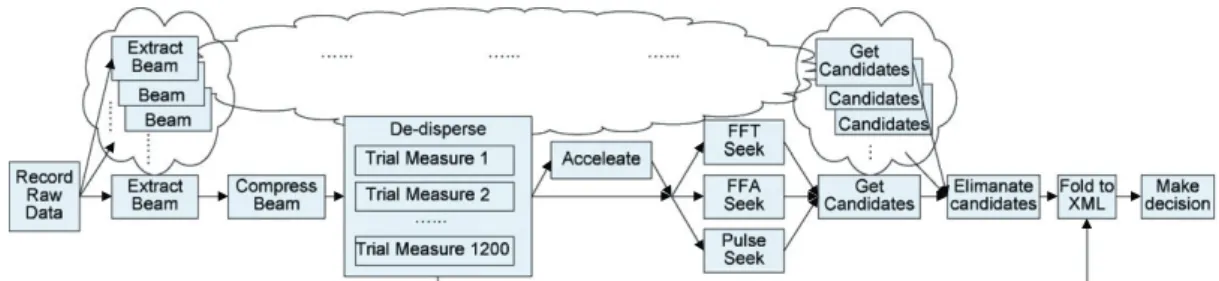
Scientific applications often need to process a large amount of data. For example, Swinburne Astrophysics group has been conducting a pulsar searching survey using the observation data from Parkes Radio Telescope (http://astronomy.swin.edu.au/pulsar/), which is one of the most famous radio telescopes in the world (http://www.parkes.atnf.csiro.au). Pulsar searching is a typical scientific application. It contains complex and time-consuming tasks and needs to process terabytes of data. Figure 1 depicts the high-level structure of a pulsar searching workflow. In the figure, we use the cloud symbol on the top to denote the parallel branches of the workflow.
At the beginning, raw signal data from Parkes Radio Telescope are recorded at a rate of one gigabyte per second by the ATNF§ Parkes Swinburne Recorder (APSR). Depending on different areas in the universe that the researchers want to conduct the pulsar searching survey, the observation time is normally from 4 min to 1 h. Recording from the telescope in real time, these raw data files have data from multiple beams interleaved. For initial preparation, different beam files are extracted from the raw data files and compressed. They are normally 1–20 GB each in size depending on the
Figure 1. Pulsar searching workflow.
observation time. The beam files contain the pulsar signals which are dispersed by the interstellar medium. De-dispersion is to counteract this effect. As the potential dispersion source is unknown, a large number of de-dispersion files will be generated with different dispersion trials. In the current pulsar searching survey, 1200 is the minimum number of the dispersion trials. Based on the size of the input beam file, this de-dispersion step will take 1–13 h to finish and generate up to 90 GB of de-dispersion files. Furthermore, for binary pulsar searching, every de-dispersion file will need another step of processing named accelerate. This step will generate the accelerated de-dispersion files with the similar size in the previous de-dispersion step. Based on the generated de-dispersion files, different seeking algorithms can be applied to search pulsar candidates, such as FFT Seeking, FFA seeking, and single pulse seeking. For a large input beam file, it will take more than 1 h to seek 1200 de-dispersion files. A candidate list of pulsars will be generated after the seeking step which is saved in a text file. Furthermore, by comparing the candidates generated from different beam files in a same time session, some interference may be detected and some candidates may be eliminated. With the final pulsar candidates, we need to go back to the beam files or the de-dispersion files to find their feature signals and fold them to XML files. Finally, the XML files will be visually displayed to researchers for making decisions on whether a pulsar has been found or not.
As described above, we can see that this pulsar searching workflow is both computation and data intensive. It is currently running on the Swinburne high-performance supercomputing facility (http://astronomy.swinburne.edu.au/supercomputing/). It needs a long execution time and a large amount of intermediate data is generated. At present, all the intermediate data are deleted after having been used, and the scientists only store the raw beam data, which are extracted from the raw telescope data. Whenever there are needs for using the intermediate data, scientists have to regenerate them based on the raw beam files. The reason that intermediate data are not stored is mainly because the supercomputer is a shared facility that cannot offer unlimited storage capacity to hold the accumulated terabytes of data. However, some intermediate data are better to be stored. For example, the de-dispersion files are frequently used intermediate data. Based on them, scientists can apply different seeking algorithms to find potential pulsar candidates. Furthermore, some intermediate data are derived from the de-dispersion files, such as the results of the seek algorithms and the pulsar candidate list. If these data are reused, the de-dispersion files will also need to be regenerated. For the large input beam files, the regeneration of the de-dispersion files will take more than 10 h. It not only delays the scientists from conducting their experiments, but also consumes a lot of computation resources. On the other hand, some intermediate data may not need to be stored. For example, the accelerated de-dispersion files, which are generated by the
accelerate step. The accelerate step is an optional step that is only for the binary pulsar searching. Not all pulsar searching processes need to accelerate the de-dispersion files, hence the accelerated de-dispersion files are not used very often. In light of this and given the large size of these data, they are not worth to store as it would be more cost effective to regenerate them from the de-dispersion files whenever they are used.
2.2. Problem analysis
Traditionally, scientific workflows are deployed on the high-performance computing facilities, such as clusters and grids. Scientific workflows are often complex with huge intermediate data generated during their execution. How to store these intermediate data is normally decided by the scientists who use the scientific workflows because the clusters and grids normally only serve for certain institutions. The scientists may store the intermediate data that are most valuable to them, based on the storage capacity of the system. However, in many scientific workflow systems, the storage capacities are limited, such as the pulsar searching workflow we introduced. The scientists have to delete all the intermediate data because of the storage limitation. This bottleneck of storage can be avoided if we run scientific workflows in the cloud.
In a cloud computing system, theoretically, the system can offer unlimited storage resources. All the intermediate data generated by scientific cloud workflows can be stored, if we are willing to pay for the required resources. However, in scientific cloud workflow systems, whether to store intermediate data or not is not an easy decision anymore.
(1) All the resources in the cloud carry certain costs, hence whether storing or generating an intermediate data set, we have to pay for the resources used. The intermediate data sets vary in size, and have different generation cost and usage rate. Some of them may often be used whereas some others may not. On one extreme, it is most likely not cost effective to store all the intermediate data in the cloud. On the other extreme, if we delete them all, regeneration of frequently used intermediate data sets imposes a high computation cost. We need a strategy to balance the regeneration cost and the storage cost of the intermediate data, to reduce the total cost of the scientific cloud workflow systems. In this paper, given the large capacity of data center and the consideration of cost effectiveness, we assume that all the intermediate data are stored within one data center with one cloud service provider, therefore, data transfer cost is not considered.
(2) However, the best trade-off of regeneration cost and storage cost may not be the best strategy for intermediate data storage. When the deleted intermediate data sets are needed, the regeneration will not only impose computation cost, but will also cause a time delay. Based on different time constraints of the scientific workflows [15, 16], users’ tolerance of this accessing delay may differ dramatically. Sometimes users may want the data to be available immediately, and sometimes they may not care about waiting for it to become available. On the one hand, one user may have different degrees of delay tolerance for different data sets. On the other hand, different users may also have different degrees of delay tolerance for a particular data set. Furthermore, one user may also have different degrees of delay tolerance for one data set in different time phases. Hence, in the strategy, we should have a parameter to indicate users’ delay tolerance, which can be set and flexibly changed by the system manager based on users’ preferences.
(3) Scientists cannot predict the usage rate of the intermediate data anymore. For a single research group, if the data resources of the applications are only used by its own scientists,
the scientists may predict the usage rate of the intermediate data and decide whether to store or delete them. However, scientific cloud workflow systems are not developed for a single scientist or institution, rather, for scientists from different institutions to collaborate and share data resources. The users of the system could be anonymous on the Internet. We must have a strategy for storing the intermediate data based on the needs of all the users that can reduce the overall cost. Hence, the data sets usage rate should be discovered and obtained from the system log, and not just manually set by the users.
Hence, for scientific cloud workflow systems, we need a strategy that can automatically select and store the most appropriate intermediate data sets. Furthermore, this strategy should be cost effective that can reduce the total cost of the systems.
3. COST-ORIENTED INTERMEDIATE DATA STORAGE IN SCIENTIFIC CLOUD WORKFLOWS
3.1. Data management in scientific cloud workflows
In a cloud computing system, application data are stored in large data centers. The cloud users visit the system via the Internet and upload the data to conduct their applications. All the application data are stored in the cloud storage and managed by the cloud computing system independent of users. As time goes on and the number of cloud users increases, the volume of data stored in the cloud will become huge. This makes the data management in cloud computing systems a very challenging job.
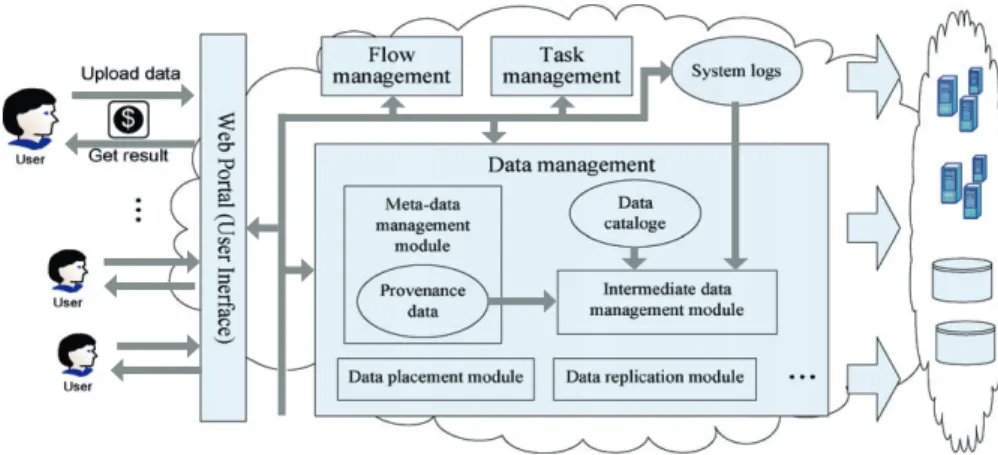
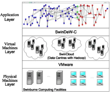
Scientific cloud workflow system is the workflow system for scientists to run their applications in the cloud. As depicted in Figure 2, it runs on cloud resources, denoted as the cloud symbol on the right, and has many differences with the traditional scientific workflow systems in data management. The most important ones are as follows: (1) For scientific cloud workflows, all the application data are managed in the cloud. Scientists can easily visit the cloud computing system via a Web portal to launch their workflows. This requires data management to be automatic; (2) A scientific cloud workflow system has a cost model. Scientists have to pay for the resources used
for conducting their applications. Hence, data management has to be cost oriented; and (3) The scientific cloud workflow system is based on the Internet, where the application data are shared and reused among the scientists world wide. For data reanalysis and regeneration, data provenance is more important in scientific cloud workflows.
In general, there are two types of data stored in the cloud storage,input dataandintermediate data including result data. First, input dataare the data uploaded by users, and in the scientific applications they also can be the raw data collected from the devices. These data are the original data for processing or analysis that are usually the input of the applications. The most important feature of these data is that if they were deleted, they could not be regenerated by the system. Second,intermediate dataare the data newly generated in the cloud computing system while the applications run. These data save the intermediate computation results of the applications that will be used in the future execution. In general, the final result data of the applications are a kind of intermediate data, because the result data in one application can also be used in other applications. When further operations apply on the result data, they become intermediate data. Hence, the intermediate data are the data generated based on either the input data or other intermediate data, and the most important feature is that they can be regenerated if we know their provenance.
For the input data, the users can decide whether they should be stored or deleted, since they cannot be regenerated once deleted. For the intermediate data, their storage status can be decided by the system, since they can be regenerated. Hence, in this paper we develop a strategy for intermediate data storage that can significantly reduce the cost of scientific cloud workflow systems.
3.2. Data provenance and intermediate data dependency graph(IDG)
Scientific workflows have many computation and data-intensive tasks that will generate many intermediate data sets of considerable size. There are dependencies existing among the intermediate data sets. Data provenance in workflows is a kind of important metadata, in which the dependencies between data sets are recorded [17]. The dependency depicts the derivation relationship between workflow intermediate data sets. For scientific workflows, data provenance is especially important, because after the execution, some intermediate data sets may be deleted, but sometimes the scientists have to regenerate them for either reuse or reanalysis [18]. Data provenance records the information about how the intermediate data sets were generated, which is very important for scientists. Furthermore, regeneration of the intermediate data sets from the input data may be very time consuming, and therefore carry a high cost. With data provenance information, the regeneration of the demanding data set may start from some stored intermediated data sets instead. In scientific cloud workflow systems, data provenance is recorded during workflow execution. Taking advantage of data provenance, we can build an IDG based on data provenance. For all the intermediate data sets once generated in the system, whether stored or deleted, their references are recorded in the IDG.
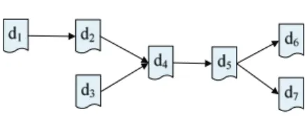
IDG is a directed acyclic graph, where every node in the graph denotes an intermediate data set. Figure 3 shows us a simple IDG, data setd1 is pointed towardd2meaning thatd1is used to generated2; data setd2andd3are pointed towardd4meaning thatd2andd3 are used together to generated4; andd5is pointed towardd6andd7meaning thatd5is used to generate eitherd6ord7 based on different operations. In an IDG, all the intermediate data sets’ provenances are recorded. When some of the deleted intermediate data sets need to be reused, we do not need to regenerate them from the original input data. With the IDG, the system can find the predecessor data sets of
Figure 3. A simple Intermediate data Dependency Graph (IDG).
the demanding data, hence they can be regenerated from their nearest existing predecessor data sets.
3.3. Data sets storage cost model
With an IDG, given any intermediate data set that ever existed in the system, we know how to regenerate it. However, in this paper, we aim at reducing the total cost of managing the intermediate data. In a cloud computing system, if the users want to deploy and run applications, they need to pay for the resources used. The resources are offered by cloud service providers, who have their cost models to charge the users. In general, there are two basic types of resources in cloud computing systems: storage and computation. Popular cloud services providers’ cost models are based on these two types of resources [19]. Furthermore, the cost of data transfer is also considered, such as in Amazon’s cost model. In [13], the authors state that a cost-effective way of doing science in the cloud is to upload all the application data to the cloud and run all the applications with the cloud services. Hence we assume that scientists upload all the input data to the cloud to conduct their experiments. Because transferring data within one cloud service provider’s facilities is usually free, the data transfer cost of managing intermediate data during workflow execution is not counted. In this paper, we define our cost model for storing the intermediate data in a scientific cloud workflow system as follows:
Cost=C+S,
where the total cost of the system,Cost, is the sum ofC, which is the total cost of computation resources used to regenerate the intermediate data, and S, which is the total cost of storage resources used to store the intermediate data. For the resources, different cloud service providers have different prices. In this paper, we use Amazon cloud services’ price as a representative, since they are well known. The prices are as follows:
• $0.15 per Gigabyte per month for the storage resources. • $0.1 per CPU hour for the computation resources.
Furthermore, we denote these two prices asCostSandCostCfor the algorithms, respectively. To utilize the data sets storage cost model, we define some important attributes for the interme-diate data sets in an IDG. For intermeinterme-diate data setdi, its attributes are denoted as: <size,flag, tp,t,,pSet,fSet,CostR>, where
• size, denotes the size of this data set;
• f lag, denotes the status whether this data set is stored or deleted in the system; • tp, denotes the time of generating this data set from its direct predecessor data sets;
• t, denotes the usage rate, which is the time between every usage of di in the system.
Figure 4. A segment of IDG.
collaboratively. However, a scientific cloud workflow system is based on the Internet with a large number of users, as we discussed before,di cannot be defined by users. It is a forecasting
value from the data set’s usage history recorded in the system logs.t is a dynamic value that changes according todi’s real usage rate in the system.
• , denotes users’ tolerance of di ’s accessing delay, which is a value between 0 and 1. The
value is set by the system manager based on users’ preference. The two extreme situations:
=0 indicates that users have no tolerance of accessing delay, which means that regardless of how largedi ’s storage cost is, it has to be stored;=1 indicates users do not care about
the accessing delay, which means that the storage status ofdi only depends on its generation
cost and storage cost to reduce the total system cost.
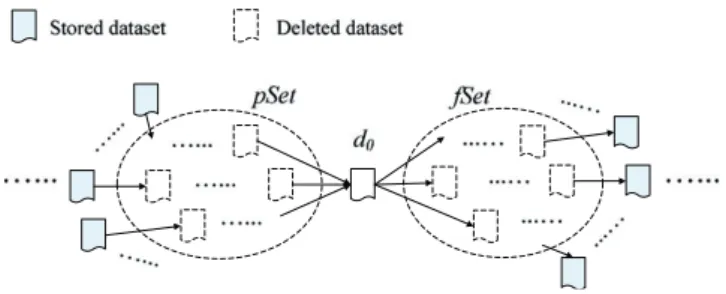
• pSet, is the set of references of all the deleted intermediate data sets in the IDG linked to
di, as shown in Figure 4. If we want to regenerate di, di.pSet contains all the data sets
that need to be regenerated beforehand. Hence, the generation cost ofdi can be denoted as: genCost(di)=(di.tp+dj∈di.pSetdj.tp)∗CostC;
• fSet, is the set of references of all the deleted intermediate data sets in the IDG that are linked by di, as shown in Figure 4. If di is deleted, to regenerate any data sets indi.fSet, we have
to regeneratedi first. In other words, if the storage status of di has changed, the generation
cost of all the data sets indi.fSetwill be affected bygenCost(di);
• CostR, is di’s cost rate, which means for the average cost per time unit of data set di in
the system, in this paper we use hour as time unit. If di is a stored data set, di.CostR= di.size∗CostS. If di is a deleted data set in the system, when we need to usedi, we have to regenerate it. Thus we divide the generation cost ofdi by the time between its usages and use this value as the cost rate ofdi in the system.di.CostR=genCost(di)/di.t. When the storage
status ofdi is changed, itsCostRwill change correspondingly.
Hence, the system cost rate of managing intermediate data is the sum of CostR of all the intermediate data sets, which isd
i∈I DG(di.CostR). Given a time duration, denoted as [T0,Tn],
the total system cost is the integral of the system cost rate in this duration as a function of timet, which is: Total_Cost= Tn t=T0 di∈I DG (di.CostR) •dt
The goal of our intermediate data management is to reduce this cost. In the following section, we will introduce a dependency-based intermediate data storage strategy, which selectively stores the intermediate data sets to reduce the total cost of the scientific cloud workflow system.
4. DEPENDENCY-BASED INTERMEDIATE DATA STORAGE STRATEGY
An IDG records the references of all the intermediate data sets and their dependencies that ever existed in the system, some data sets may be stored in the system, and others may be deleted. Our dependency-based intermediate data storage strategy is developed based on the IDG, and applied at workflow runtime. During workflows execution, when new data sets are generated in the system, their information is added to the IDG for the first time, and then when they have finished being used, the strategy will decide whether they should be stored or deleted. For the stored intermediate data sets, the strategy will periodically check whether they still need to be stored. For the deleted intermediate data sets, when they are regenerated, the strategy will check whether circumstances have changed, and decide whether they should now be stored. Deciding whether to store or delete an intermediate data set is based on comparing its generation cost rate and storage cost rate, where the storage cost rate have to multiply the delay tolerance parameter beforehand, in order to reflect users’ preference of the accessing delay of that data set. Our strategy can dynamically store the necessary intermediate data sets during workflow execution with the acceptable data accessing delay, which means deleting any stored data sets in the system would bring an increase of system cost. The strategy contains three algorithms described in this section. Furthermore, a data set’s usage ratet, which is used for the calculation of data set’s generation cost rate, is obtained from the system log. As it is an estimated value, there would be some forecasting inaccuracy in it. At the end of this section, we will analyze forecasting inaccuracy’s impact on our strategy.
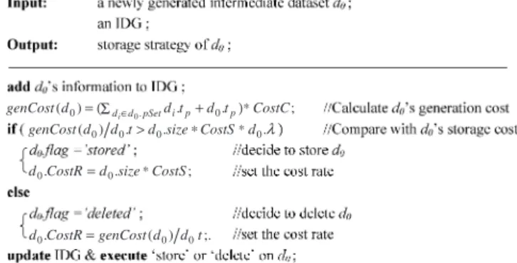
4.1. Algorithm for deciding newly generated intermediate data sets’ storage status
Supposed0is a newly generated intermediate data set.
First, we add its information to the IDG. We find the provenance data sets of d0 in the IDG, and add edges pointing tod0from these data sets. Then we initialize its attributes. Asd0does not have a usage history yet, we use the average value in the system as the initial value ofd0’s usage rate.
Next, we check whetherd0needs to be stored or not. Asd0is newly added in the IDG, it does not have successor data sets in the IDG, which means no intermediate data sets are derived from
d0 at this moment. For deciding whether to store or delete d0, we only compare the generation cost rate of d0 itself and its storage cost rate multiplied by the delay tolerance parameter , which are genCost(d0)/d0.t and d0.size∗CostS∗d0.. If the cost of generation is larger than the cost of storing it, we save d0 and setd0.CostR=d0.size∗CostS, otherwise we delete d0 and set
d0.CostR=genCost(d0)/d0.t. The algorithm is shown in Figure 5.
In this algorithm, we guarantee that all the intermediate data sets chosen to be stored are necessary, which means that deleting any one of them would increase the cost of the system, since they all have a higher generation cost than storage cost.
4.2. Algorithm for managing stored intermediate data sets
The usage ratet of a data set is an important parameter that determines its storage status. Ast is a dynamic value that may change at any time, we have to dynamically check whether the stored intermediate data sets in the system still need to be stored.
For an intermediate data set d0 that is stored in the system, we set a threshold timet, where
( . . ) ; ) (d0 . d t d0t CostC genCost = d∈d pSet i p+ p∗ λ . . . ) (d0 d0t d0size CostS d0 genCost > ∗ ∗ ; . . 0
0CostR d size CostS
d = ∗ ;. ) ( . 0 0 0CostR genCostd d t d =
Figure 5. Algorithm for handling newly generated data sets.
(
. .)
; ) ( 0 . 0 0 d t d t CostC d genCost d d pSet i p p i + = ∈ ; . ) ( . 0 0 0CostR genCostd d t d = ; . ) ( ..CostR d CostR genCostd0 d t
di = i + i
( ( ) .) . .
. )
( 0 0 . 0 0 0
0 genCostd d t d size CostS d t d d genCost d d fSet i i > + ∈ ; . ' T d0t T= + t
Figure 6. Algorithm for checking stored intermediate data sets.
stored in the system with the cost of generating it. Ifd0has not been used for the time oft, we will check whether it should be stored anymore.
If we delete stored intermediate data setd0, the system cost rate is reduced byd0’s storage cost rate, which is d0.size∗CostS. Meanwhile, the increase of the system cost rate is the sum of the generation cost rate ofd0itself, which isgenCost(d0)/d0.t, and the increased generation cost rates of all the data sets in d0.fSet caused by deletingd0, which is
di∈d0.fSet(genCost(d0)/di.t). We
compared0’s storage cost rate and generation cost rate to decide whetherd0should be stored or not. The detailed algorithm is shown in Figure 6.
Lemma 1
The deletion of stored intermediate data set d0 in the IDG does not affect the stored data sets adjacent tod0, where the stored data sets adjacent tod0 means the data sets that directly link to
d0ord0.pSet, and the data sets that are directly linked byd0 ord0.fSet.
Proof
(1) Suppose dp is a stored data set directly linked to d0 or d0.pSet. As d0 is deleted, d0 and d0.fSet are added to dp.fSet. Thus the new generation cost rate of dp in the system is genCost(dp)/dp.t+di∈dp.fSet∪d0∪d0.fSet(genCost(dp)/di.t), and it is larger than before,
which was genCost(dp)/dp.t+di∈dp.fSet(genCost(dp)/di.t). Hence dp still needs to be
stored.
(2) Suppose df is a stored data set directly linked by d0 or d0.fSet. As d0 is deleted, d0 and d0.pSet are added to df.pSet. Thus the new generation cost of df is genCost(df)=
(df.tp+
di∈df.pSet∪d0∪d0.pSetdi.tp)∗CostC, and it is larger than before, which was
genCost(df)=(df.tp+di∈df.pSetdi.tp)∗CostC. Because of the increase of genCost(df),
the generation cost rate ofdf in the system is larger than before, which wasgenCost(df)/df.t
+di∈df.fSet(genCost(df)/di.t). Hencedf still needs to be stored.
Because of (1) and (2), the Lemma holds.
By applying the algorithm of checking the stored intermediate data sets, we can still guarantee that all the data sets we have kept in the system are necessary to be stored. Furthermore, when the deleted intermediate data sets are regenerated, we also need to check whether to store or delete them as discussed next.
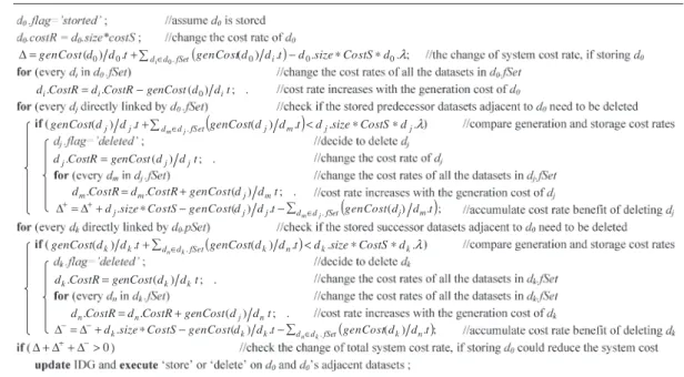
4.3. Algorithm for deciding the regenerated intermediate data sets’ storage status
IDG is a dynamic graph where the information about new intermediate data sets may join at anytime. Although the algorithms in the above two subsections can guarantee that the stored intermediate data sets are all necessary, these stored data sets may not be the most cost effective. Initially deleted intermediate data sets may need to be stored as an IDG expands. Supposed0 to be a regenerated intermediate data set in the system, which has been deleted before. After having been used, we recalculated0’s storage status, as well as the stored data sets adjacent to d0 in the IDG.
Theorem
If regenerated intermediate data setd0is stored, only the stored data sets adjacent tod0in the IDG may need to be deleted to reduce the system cost.
Proof
(1) Supposedp is a stored data set directly linked tod0 or d0.pSet. As d0 is stored, d0 and
d0.fSet need to be removed from dp.fSet. Thus the new generation cost rate ofdp in the
system isgenCost(dp)/dp.t+di∈dp.fSet−d0−d0.fSet(genCost(dp)/di.t), and it is smaller than
before, which wasgenCost(dp)/dp.t+di∈dp.fSet(genCost(dp)/di.t). If the new generation
cost rate is smaller than the storage cost rate of dp, dp would be deleted. The remainder
of the stored intermediate data sets are not affected by the deletion of dp, because of the
Lemma introduced before.
(2) Suppose df is a stored data set directly linked by d0 or d0.fSet. As d0 is stored, d0 and d0.pSet need to be removed from df.pSet. Thus the new generation cost of df is genCost(df)=(df.tp+di∈df.pSet−d0−d0.pSetdi.tp)∗CostC, and it is smaller than before,
which was genCost(df)=(df.tp+
di∈df.pSetdi.tp)∗CostC. Because of the reduction of
genCost(df), the generation cost rate of df in the system is smaller than before, which
was genCost(df)/df.t+
di∈df.fSet(genCost(df)/di.t). If the new generation cost rate is
Figure 7. Algorithm for checking deleted intermediate data sets.
intermediate data sets are not affected by the deletion ofdf, because of the Lemma
intro-duced before.
Because of (1) and (2), the theorem holds.
If we store regenerated intermediate data setd0, the cost rate of the system increases withd0’s storage cost rate, which is d0.size∗CostS. Meanwhile, the reduction of the system cost rate may be resulted from three aspects: (1) the generation cost rate ofd0itself, which isgenCost(d0)/d0.t; (2) the reduced generation cost rates of all the data sets in d0.fSetcaused by storingd0, which is
di∈d0.fSet(genCost(d0)/di.t); and (3) as indicated in the Theorem, some stored data sets adjacent
tod0may be deleted that reduces the cost to the system. We will compare the increase and reduction of the system cost rate to decide whether d0 should be stored or not. The detailed algorithm is shown in Figure 7.
By applying the algorithm of checking the regenerated intermediate data sets, we can not only guarantee that all the data sets we have kept in the system are necessary to be stored, but also that any changes of the data sets’ storage status will reduce the total system cost.
4.4. Impact analysis of forecasting inaccuracy
As stated in Section 3, the data sets usage ratet is an estimated value that is obtained from the system log. Hence, there might be some forecasting inaccuracy. However, how to precisely forecast the data sets usage rate from the system log is out of this paper’s scope. Here we only analyze the impact of the forecasting inaccuracy on our strategy.
It is logical that the performance of our strategy would be affected by the forecasting inaccuracy of the data sets usage rate, since the storage status of the data sets may be miscalculated due to inaccuracy. However, not all the forecasting inaccuracy will cause miscalculation of the data sets storage status.
Supposed0is a data set that should be deleted in the system, which meansd0’s generation cost rate is smaller than its storage cost rate, i.e.
genCost(d0)/d0.t+
di∈d0.fSet
(genCost(d0)/di.t)<d0.size∗CostS∗d0.
If d0 has a negative forecasting inaccuracy of usage rate, which means the forecasted usage ratete is longer than the real usage ratet, the calculation of storage status will not be affected by
the forecasting inaccuracy. This is because with a negative forecasting inaccuracy, the inaccurate generation cost rate calculated is smaller than the real one, and also smaller than the storage cost rate. If we wantd0’s storage status miscalculated such that it will be stored,d0must have a positive forecasting inaccuracy of usage rate, and furthermore guarantee thatd0’s generation cost rate is larger than its storage cost rate, i.e.
d0.size∗CostS∗d0.<genCost(d0)/d0.te+ di∈d0.fSet
(genCost(d0)/di.t)
Hence, the chance that forecasting inaccuracy would impact the storage status of data sets is less than 50%. This is because:
(1) Ifd0is a data set that should be deleted in the system, only the positive forecasting inaccuracy of its usage rate will affect its storage status, and this inaccurate usage rate must further satisfy the following condition:
te<genCost(d0)/(d0.size∗CostS∗d0.−
di∈d0.fSet
(genCost(d0)/di.t))
(2) Similarly, ifd0is a data set that should be stored in the system, only the negative forecasting inaccuracy of its usage rate will affect its storage status, and this inaccurate usage rate must further satisfy the following condition:
te>genCost(d0)/(d0.size∗CostS∗d0.−
di∈d0.fSet
(genCost(d0)/di.t)).
In the following section, we will use simulation results to further illustrate the impact of the data sets usages forecasting inaccuracy in our strategy from where no significant impact is observed.
5. EVALUATION
The intermediate data storage strategy proposed in this paper is generic. It can be used in any scientific workflow applications. In this section, we demonstrate the simulation results that we conduct on the SwinCloud system [20]. In the beginning, we use random workflows and data sets to demonstrate the general performance of our strategy. Then we deploy the strategy to the pulsar searching workflow described in Section 2, and use the real-world statistics to demonstrate how our strategy works in storing the intermediate data sets of the pulsar searching workflow.
Figure 8. Structure of simulation environment.
5.1. Simulation environment and strategies
Figure 8 shows the structure of our simulation environment. SwinCloud is a cloud computing simulation environment built on the computing facilities in Swinburne University of Tech-nology and takes advantage of the existing SwinGrid system [21]. We install VMWare software (http://www.vmware.com/) on SwinGrid, so that it can offer unified computing and storage resources. By utilizing the unified resources, we set up data centers that can host applications. In the data centers, Hadoop (http://hadoop.apache.org/) is installed that can facilitate the Map-Reduce computing paradigm and distributed data management. SwinDeW-C (Swinburne Decentralized Workflow for Cloud) [20] is a cloud workflow system developed based on SwinDeW [22] and SwinDeW-G [21]. It is currently running on SwinCloud that can interpret and execute workflows, send and retrieve, save and delete data in the virtual data centers. Through a user interface at the application level, which is a Web portal, we can deploy workflows and upload application data to the cloud. In the simulation, we facilitate our strategy in SwinDeW-C to manage the intermediate data sets in the simulation cloud.
To evaluate the performance of our strategy, we run five simulation strategies together and compare the total cost of the system. The strategies are: (1) store all the intermediate data sets in the system; (2) delete all the intermediate data sets, and regenerate them whenever needed; (3) store the data sets that have high generation cost; (4) store the data sets that are most often used; and (5) our strategy to dynamically decide whether a data set should be stored or deleted.
We have run a large number of simulations with different parameters to evaluate the performance of our strategy. Owing to space limits, we only evaluate some representative results here.
5.2. Random simulations and results
To evaluate the overall performance of our strategy, we run a large number of random simulations with the five strategies introduced above. In the random simulations, we use randomly generated
Total Cost of 50 Days 0 50 100 150 200 250 300 1 Days Cost ($)
Store all datasets
Store none
Store high creation cost datasets
Store often used datasets
Dependency based storage
3 5 7 9 11 13 15 17 19 21 23 25 27 29 31 33 35 37 39 41 43 45 47 49
Figure 9. Total system cost of random simulation case with Amazon’s cost model.
workflows to construct the IDG, and give every intermediate data set random size, generation time, usage rate, delay tolerance, and then run the workflows. We compare the total system cost over 50 days of the five strategies, which shows the reduction of the total system cost of our strategy.
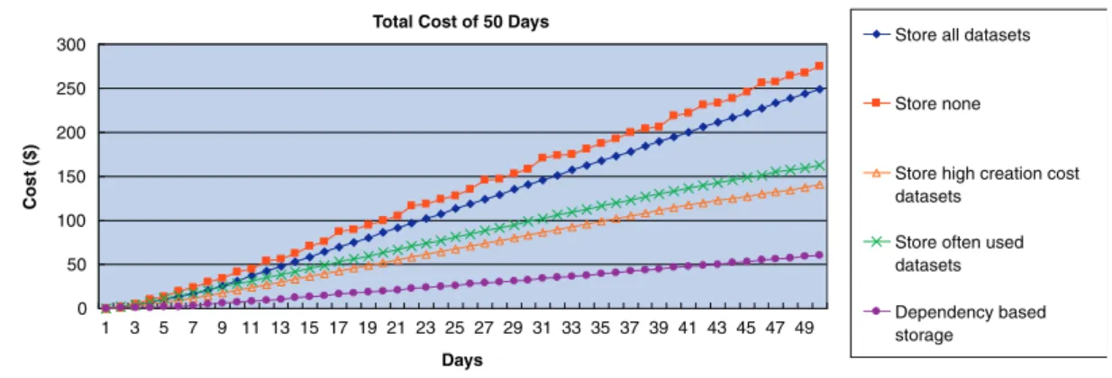
We pick one representative test case. In this case, we let the workflow randomly generate 20 intermediate data sets, each with a random size from 1–100 GB. The generation time is also random, from 1min to 60 mins. The usage rate is again random ranging from 1–10 days. We further assume that users are tolerant with the computation delay. The prices of cloud services follow Amazon’s cost model which can be viewed as a specific case of our cost model presented in Section 3, i.e. $0.1 per CPU hour for computation and $0.15 per gigabyte per month for storage. Figure 9 shows the total cost of the system over the 50 days.
As indicated in Figure 9, we can draw the conclusion that (1) neither storing all the intermediate data sets nor deleting them all is a cost-effective method of intermediate data storage; (2) the two static strategies of ‘store high generation cost data sets’ and ‘store often used data sets’ are in the middle band in reducing the total system cost; (3) our dependency-based strategy performs as the most cost effective method for storing the intermediate data sets. It reduces the system cost by 75.9% in comparison to the ‘store all’ strategy; 78.2% to the ‘store none’ strategy; 57.1% to the ‘store high generation cost data sets’ strategy; and 63.0% to the ‘store often used data sets’ strategy, respectively.
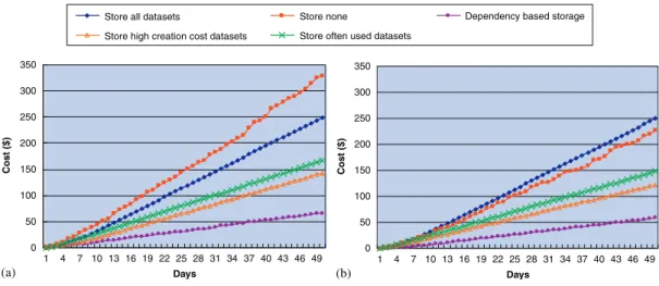
As in our strategy, the intermediate data set’s usage rate is a forecast value based on the system log. There may well exist some inaccuracies in this value. The simulation taking this into account demonstrates the impact of forecast inaccuracy on our strategy. We set 20% positive and negative forecast inaccuracy to the usage rates of the intermediate data sets and conduct another two sets of simulation, the results of which are shown in Figure 10. We can clearly see that the costs with the ‘store none’ strategy have shifted about 20% compared to the result in Figure 9. However the ‘store all’ strategy is not influenced by the forecast inaccuracies. The forecast inaccuracy has little impact on our strategy, where it is still the most cost-effective one among the five strategies.
Next, we add the delay tolerance parameter in our simulation. We set =70% and run the simulation with the same settings as that in Figure 9. The results are demonstrated in Figure 11. We can see that with the users’ preference of less delay tolerance, the system cost increases. This is because our strategy has chosen more data sets to store in the system.
Total Cost of 50 Days
Store all datasets Store none Dependency based storage Store high creation cost datasets Store often used datasets
0 50 100 150 200 250 300 350 1 Days Cost ($) 0 50 100 150 200 250 300 350 Days Cost ($) 4 7 10 13 16 19 22 25 28 31 34 37 40 43 46 49 1 4 7 10 13 16 19 22 25 28 31 34 37 40 43 46 49 (a) (b)
Figure 10. System cost with forecasting inaccuracy in data sets usage rate: (a) Usage rate 20% higher than forecasted and (b) usage rate 20% lower than forecasted.
Total Cost of 50 Days
0 50 100 150 200 250 300 1 3 5 7 9 11 13 15 17 19 21 23 25 27 29 31 33 35 37 39 41 43 45 47 49 Days Co s t ( $ )
Store all datasets
Store none
Store high creation cost datasets
Store often used datasets Dependency based storage with =70% Dependency based storage
Figure 11. System cost with delay tolerance parameter added.
5.3. Pulsar case simulations and results
The random simulations demonstrate the general performance of our strategy. Next we utilize it for the pulsar searching workflow introduced in Section 2 and show how the strategy works in a specific real scientific application.
In the pulsar example, during the workflow execution, six intermediate data sets are generated. The IDG of this pulsar searching workflow is shown in Figure 12, as well as the sizes and generation times of these intermediate data sets. The generation times of the data sets are from running this workflow on Swinburne supercomputer, and for simulation, we assume that in the cloud computing system, the generation times of these intermediate data sets are the same. Furthermore, we assume that the prices of cloud services follow Amazon’s cost model.
Figure 12. IDG of pulsar searching workflow. Total cost of 50 days
0 10 20 30 40 50 1 3 5 7 9 11 13 15 17 19 21 23 25 27 29 31 33 35 37 39 41 43 45 47 49 Days Co s t ( $ ) Store all Store none
Store high generation cost datasets Store often used datasets Dependency based strategy
Figure 13. Total cost of pulsar searching workflow with Amazon’s cost model.
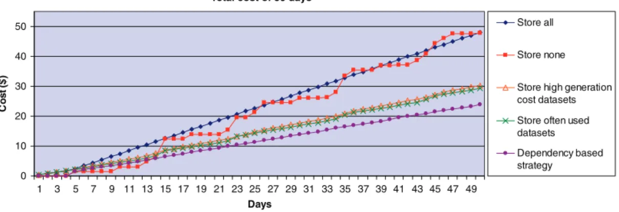
We run the simulations based on the estimated usage rate of every intermediate data set. From Swinburne astrophysics research group, we understand that the ‘de-dispersion files’ are the most useful intermediate data set. Based on these files, many accelerating and seeking methods can be used to search pulsar candidates. Hence, we set the ‘de-dispersion files’ to be used once in every 4 days, and the remainder of the intermediate data sets to be used once in every 10 days. Based on this setting, we run the abovementioned five simulation strategies and calculate the total costs of the system for ONE branch of the pulsar searching workflow of processing ONE piece of observation data in 50 days as shown in Figure 13.
From Figure 13 we can see that (1) the cost of the ‘store all’ strategy is a straight line, because in this strategy, all the intermediate data sets are stored in the cloud storage that is charged at a fixed rate, and there is no computation cost required; (2) the cost of the ‘store none’ strategy is a fluctuated line because in this strategy all the costs are computation costs of regenerating intermediate data sets. For the days that have fewer requests of the data, the cost is lower, otherwise, the cost is higher; (3–5) in the remaining three strategies, the cost lines are only a little fluctuated and the cost is much lower than the ‘store all’ and ‘store none’ strategies in the long term. This is because the intermediate data sets are partially stored.
As indicated in Figure 13 we can draw the same conclusions as we did for the random simulations, that (1) neither storing all the intermediate data sets nor deleting them all is a cost-effective way for intermediate data storage; (2) our dependency-based strategy performs the most cost effective to store the intermediate data sets in the long term.
Furthermore, back to the pulsar searching workflow example, Table I shows how the five strategies store the intermediate data sets in detail.
Table I. Pulsar searching workflow’s intermediate data sets storage status in five strategies.
Data sets
Extracted De-dispersion Accelerated Seek Pulsar XML files Strategies beam files de-dispersion files results candidates XML files
Store all Stored Stored Stored Stored Stored Stored
Store none Deleted Deleted Deleted Deleted Deleted Deleted
Store high generation cost data sets
Deleted Stored Stored Deleted Deleted Stored
Store often used data sets
Deleted Stored Deleted Deleted Deleted Deleted
Dependency based strategy
Deleted Stored (was deleted initially)
Deleted Stored Deleted Stored
As the intermediate data sets of this pulsar searching workflow are not complicated, we can do some intuitive analyses on how to store them. For the accelerated de-dispersion files, although its generation cost is quite high, comparing to its huge size, it is not worth to store them in the cloud. However, in the strategy of ‘store high generation cost data sets’, the accelerated de-dispersion files are chosen to be stored. Furthermore, for the final XML files, they are not used very often, but compared to the high generation cost and small size, they should be stored. However, in the strategy of ‘store often used data sets’, these files are not chosen to be stored. Generally speaking, our dependency-based strategy is the most appropriate strategy for the intermediate data storage which is also dynamic. From Table I we can see that our strategy did not store the de-dispersion files at the beginning, but stored them after their regeneration. In our strategy, every storage status change of the data sets would reduce the total system cost rate, where the cost can be gradually close to the minimum cost of system.
One important factor that affects our dependency-based strategy is the usage rate of the inter-mediate data sets. In a system, if the usage rage of the interinter-mediate data sets is very high, the generation cost of the data sets is very high, correspondingly these intermediate data sets tend more to be stored. On the contrary, in a very low intermediate data sets usage rate system, all the data sets tend to be deleted. The simulation of Figure 13, we set the data sets usage rate on the borderline that makes the total cost equivalent to the strategies of ‘store all’ and ‘store none’. Under this condition, the intermediate data sets have no tendency to be stored or deleted, which can objectively demonstrate our strategy’s effectiveness on reducing the system cost. Next we will also demonstrate the performance of our strategy in situations under different usage rates of the intermediate data sets.
Figure 14(a) shows the cost of the system with the usage rate of every data set doubled in the pulsar workflow. From the figure we can see that, when the data sets usage rates are high, the strategy of ‘store none’ becomes highly cost ineffective, because the frequent regeneration of the intermediate data sets causes a very high cost to the system. In contrast, our strategy is still the most cost-effective one where the total system cost increases only slightly. It is not very much influenced by the data sets usage rates. For the ‘store all’ strategy, although it is not influenced by the usage rate, its cost is still very high. The remaining two strategies are in the midband. They are influenced by the data sets usage rates more, and their total costs are higher than our strategy.
Total cost of 50 days
Store all Store none Store high generation cost datasets Store often used datasets Dependency based strategy
0 10 20 30 40 50 Days Co s t ( $ ) 0 10 20 30 40 50 Days C o s t ($ ) 1 4 7 10 13 16 19 22 25 28 31 34 37 40 43 46 49 1 4 7 10 13 16 19 22 25 28 31 34 37 40 43 46 49 (a) (b)
Figure 14. Cost of pulsar searching workflow with different intermediate data sets usage rates: (a) High intermediate datasets usage rate; (b) Low intermediate datasets usage rates.
Total cost of 50 days
0 10 20 30 40 50 Days C o s t ($ )
Store all Store none Store high generation cost datasets Store often used datasets Dependency based strategy
0 10 20 30 40 50 Days Co s t ( $ ) 1 4 7 10 13 16 19 22 25 28 31 34 37 40 43 46 49 1 4 7 10 13 16 19 22 25 28 31 34 37 40 43 46 49 (a) (b)
Figure 15. Cost of pulsar searching workflow with forecast inaccuracy in intermediate data sets usage rates: (a) Usage rate 20% higher than forecasted; (b) Usage rate 20% lower than forecasted.
Figure 14(b) shows the cost of the system with the usage rate of every data set halved in the pulsar workflow. From this figure we can see that, in the system with a low intermediate data sets usage rate, the ‘store all’ strategy becomes highly cost ineffective, and the ‘store none’ strategy becomes relatively cost effective. Again, our strategy is still the most cost-effective one among the five strategies.
The more intermediate data sets are stored in the system, the less the cost of the system is influenced by the data sets usage rate. As in our strategy, the intermediate data sets usage rate is a forecast value based on the system log. There may well be some inaccuracy existing. The simulations taking this into account demonstrate the influence of forecast inaccuracy on our strategy. We set 20% positive and negative forecast inaccuracy the usage rates of the intermediate data sets and conduct another two sets of simulations. The results are depicted in Figure 15. We can clearly
see that the costs in the ‘store none’ strategy have shifted about 20% compared to the result in Figure 13. However the ‘store all’ strategy is not influenced by the forecast inaccuracy. For the remaining three strategies, the forecast inaccuracy has little impact on them, whereas our strategy is still the most cost-effective one among the five strategies.
From all the simulations we have done on the pulsar searching workflow, we find that depending on different intermediate data sets usage rates, our strategy can reduce the system cost by 46.3–74.7% in comparison to the ‘store all’ strategy; 45.2–76.3% to the ‘store none’ strategy; 23.9–58.9% to the ‘store high generation cost data sets’ strategy; and 32.2–54.7% ‘store often used data sets’ strategy, respectively.
Based on the simulation results demonstrated in this section, we can reach the conclusion that our intermediate data storage strategy has a good performance. By automatically selecting the valuable data sets to store, our strategy can significantly reduce the total cost of the pulsar searching workflow.
6. DISCUSSION
As cloud computing is such a fast growing market, different cloud service providers will be avail-able. In the future, we will be able to flexibly select service providers to conduct our applications based on their pricing models. An intuitive idea is to incorporate different cloud service providers in our applications, where we can store the data with the provider who has a lower price in storage resources, and choose the provider who has lower price of computation resources to run the computation tasks. However, at present, it is not practical to run scientific workflow applications among different cloud service providers, because of the following reasons:
(1) The application data in scientific workflows are usually very large in size. They are too large to be transferred efficiently via the Internet. Owing to bandwidth limitations of the Internet, in today’s scientific projects, delivery of hard disks is a very common way to transfer application data, and it is also considered to be the most efficient way to transfer terabytes of data [23]. Nowadays, express mail delivery companies can deliver the hard disks nationwide by the end of the next day and world wide in 2 or 3 days, by contrast, transferring one terabyte data via Internet will take more than 10 days at a speed of 1 MB/s. To break the bandwidth limitation, some institutions set up dedicated fibers to transfer data. For example, Swinburne University of Technology has built a fiber to Parkes with gigabit bandwidth. However, it is mainly used for transferring gigabytes of data. To transfer terabytes of data, scientists still prefer to ship hard disks. Furthermore, building fiber connections is still expensive, and they are not wildly used in the Internet. Hence, transfer-ring scientific application data between different cloud service providers via Internet is not efficient.
(2) Cloud service providers place high cost on data transfer in and out of their data centers, in contrast, data transfer within a cloud service provider’s data centers is usually free. For example, the data transfer price of Amazon cloud service is: $0.1 per GB of data transferred in and $0.17 per GB of data transferred out. Compared to the storage price of $0.15 per GB per month, the data transfer price is relatively high, such that finding a cheaper storage cloud service provider and transferring data out may not be cost effective. In cloud service providers’ position, they charge a high price on data transfer not only because of the
bandwidth limitation, but also as a business strategy. As data are deemed as an important resource today, cloud service providers want users to keep all the application data in their storage cloud. For example, Amazon made a promotion that places a zero price on data transferred into its data centers, until June 30. 2010. This means that users can upload their data to Amazon’s cloud storage for free. However, the price of data transfer out of Amazon is still the same.
Given the two points discussed above, the most efficient and cost-effective way to run scientific applications in the cloud is to keep all the application data and run the workflows with one cloud service provider, where the similar conclusion is also stated in [13]. Hence, in the strategy stated in this paper, we did not take data transfer cost into consideration. However, some scientific applications have to run in a distributed manner [24, 25], because the required data sets are distributed and have fixed locations. In these cases, data transfer is inevitable, and data placement strategy [26] would be needed to reduce the data transfer cost.
7. RELATED WORKS
In the grid era, research of economics-based resource management had already emerged [27]. Comparing to the distributed computing systems like cluster and grid, a cloud computing system has a cost benefit [23]. Assunção et al. [28] demonstrate that cloud computing can extend the capacity of clusters with a cost benefit. Using Amazon clouds’ cost model and BOINC volunteer computing middleware, the work in [29] analyzes the cost benefit of cloud computing versus grid computing. The idea of doing science in the cloud is not new. Scientific applications have already been introduced to cloud computing systems. The Cumulus project [12] introduces a scientific cloud architecture for a data center, and the Nimbus [11] toolkit can directly turn a cluster into a cloud which has already been used to build a cloud for scientific applications. In terms of the cost benefit, the work by Deelman et al. [13] also apply Amazon clouds’ cost model and demonstrate that cloud computing offers a cost-effective way to deploy scientific applications. The above works mainly focus on the comparison of cloud computing systems and the traditional distributed computing paradigms, which shows that applications running in the cloud have cost benefits. However, our work investigates how to reduce the cost if we run scientific workflows in the cloud. In [13], Deelman et al. present that storing some popular intermediate data can save the cost in comparison to always regenerating them from the input data. In [5], Adams et al.
propose a model to represent the trade-off of computation cost and storage cost, but have not given any strategy to find this trade-off. In our paper, an innovative intermediate data storage strategy is developed to reduce the total cost of scientific cloud workflow systems by finding the trade-off of computation cost and storage cost. This strategy is based on the dependency of workflow intermediate data, and can automatically select the appropriate intermediate data sets to store by comparing their generation cost rate and storage cost rate. Furthermore, the strategy also takes the users’ tolerance of computation delays into consideration and is not strongly impacted by the forecasting inaccuracy of data sets’ usages.
The study of data provenance is important in our work. Owing to the importance of data provenance in scientific applications, much research about recording data provenance of the system has been done [30, 31]. Some of them are especially for scientific workflow systems [30]. Some popular scientific workflow systems, such as Kepler [2], have their own system to record provenance
during the workflow execution [32]. In [33], Osterweil et al. present how to generate a Data Derivation Graph (DDG) for the execution of a scientific workflow, where one DDG records the data provenance of one execution. Similar to the DDG, our IDG is also based on the scientific workflow data provenance, but it depicts the dependency relationships of all the intermediate data in the system. With the IDG, we know where the intermediate data are derived from and how to regenerate them.
8. CONCLUSIONS AND FUTURE WORK
In this paper, based on an astrophysics pulsar searching workflow, we examined the unique features of intermediate data management in scientific cloud workflow systems and developed a novel cost-effective strategy that can automatically and dynamically select the appropriate intermediate data sets of a scientific workflow to store or delete in the cloud. The selection also takes users’ tolerance of data accessing delay into consideration. The strategy can guarantee that the stored intermediate data sets in the system are all necessary, and can dynamically check whether the regenerated data sets need to be stored, and if so, adjust the storage strategy accordingly. The simulation results of utilizing this strategy in both general random workflows and the specific real world pulsar searching workflow indicate that our strategy can significantly reduce the total cost of the scientific cloud workflow systems.
Our current work assumes that all the application data are stored with one cloud service provider as discussed in Section 6. However, sometimes scientific workflows have to run in a distributed manner, since some application data are distributed and may have fixed locations. In these cases, data transfer is inevitable. In the future, we will further develop some data placement strategies to reduce data transfer among data centers. In addition, models of estimating data sets usage rates need to be studied, so that the cost calculated by our data sets storage cost model can be more accurate to the real cost in the cloud.
ACKNOWLEDGEMENTS
The research work reported in this paper is partly supported by Australian Research Council under Linkage Project LP0990393. The authors are also grateful for the discussions with Dr W. van Straten and L. Levin from the Swinburne Centre for Astrophysics and Supercomputing on the pulsar searching process, as well as the simulation work and English proof reading assistance from B. Gibson.
REFERENCES
1. Deelman E, Blythe J, Gil Y, Kesselman C, Mehta G, Patil S, Su M-H, Vahi K, Livny M. Pegasus: Mapping scientific workflows onto the grid.European Across Grids Conference, Nicosia, Cyprus, 2004; 11–20. 2. Ludascher B, Altintas I, Berkley C, Higgins D, Jaeger E, Jones M, Lee EA. Scientific workflow management
and the Kepler system.Concurrency and Computation:Practice and Experience, 2005; 1039–1065.
3. Oinn T, Addis M, Ferris J, Marvin D, Senger M, Greenwood M, Carver T, Glover K, Pocock MR, Wipat A, Li P. Taverna: A tool for the composition and enactment of bioinformatics workflows. Bioinformatics 2004;
20:3045–3054.
4. Deelman E, Chervenak A. Data management challenges of data-intensive scientific workflows.IEEE International Symposium on Cluster Computing and the Grid(CCGrid’08), Lyon, France, 2008; 687–692.
5. Adams I, Long EDD, Miller LE, Pasupathy S, Storer WM. Maximizing efficiency by trading storage for computation.Workshop on Hot Topics in Cloud Computing(HotCloud’09), San Diego, CA, 2009; 1–5.