TWO-DIMENSIONAL WAVE RUN-UP INUNDATION ANALYSIS
Jeffrey A. Oskamp1and Ahmed “Jemie” A. Dababneh2
1
Engineering Associate, RIZZO Associates, USA 2
Managing Principal, RIZZO Associates, USA
ABSTRACT
Due to the complex nature of wave run-up (wind-generated waves approaching a shoreline), characterization of run-up inundation can be difficult. For example, if waves during a storm surge event inundate around a complex network of structures, it is difficult (if not impossible) to evaluate inundation extents/depths and associated loadings on structures using existing empirical run-up equations.
A method was developed to combine the application of empirical run-up equations with two-dimensional hydrodynamic modelling to characterize inundation of waves. A synthetic wave field is developed for input to the hydrodynamic model. The height of the synthetic wave field is calibrated to ensure that the run-up height in the model matches the run-up height indicated by an empirical run-up equation for specified design incident wave conditions. The calibrated synthetic wave field is used as the input to a detailed model that simulates inundation around structures. The model output can provide information about inundation depths and velocities, which support a detailed evaluation of loadings exerted on inundated structures.
A validation of this method is provided by comparing the results to a more computationally intensive numerical model. This methodology provides a way to estimate the extent of wave run-up inundation in circumstances where some other two-dimensional run-up simulation techniques are too computationally intensive, empirical run-up equations are not sufficient, and physical modelling is not feasible.
INTRODUCTION
Advancing computer technologies provide new opportunities to solve complex coastal engineering problems. Computers can provide benefit for practical engineering application for evaluating the dynamics of wave breaking and run-up in nearshore areas. Unfortunately, the computational methods that are most applicable for characterizing wave dynamics in the surf zone remain computationally intensive and are often only economically viable for large projects or in research settings.
State-of-the-art modelling software for characterizing nearshore wave dynamics is typically based on Boussinesq-type equations, e.g., FUNWAVE-TVS (Tehranirad et al., 2011). Recently, a somewhat less computationally intense method has been proposed based on an extension of the Non-Linear Shallow Water (NLSW) equations (Zijlema and Stelling, 2008). The NLSW equations are commonly used for many over-land flow flooding applications, including tsunami inundation analysis (Zijlema et al., 2011). The inclusion of the non-hydrostatic pressure term in the NLSW equations provides increased accuracy necessary for simulating breaking waves in the surf zone (Zijlema et al., 2008; Smit et al., 2013). However, the computational burden of a non-hydrostatic NLSW equation model remains significantly higher than a hydrostatic NLSW equation model (approximately three times higher for cases considered in this study).
and Stockdon et al. [2006]), allowing for determination of wave run-up inundation extents (e.g., behind structures) and the associated hydrodynamic and hydrostatic forces.
The proposed method involves a synthesis of numerical hydrodynamic modelling with traditional coastal engineering wave run-up equations. A hydrostatic NLSW equation model (which, as discussed above, accounts for some, but not all of the physical processes present in the nearshore zone) is coupled with run-up heights estimated from empirical run-up equations. The empirically based run-up heights can be used to calibrate the hydrostatic NLSW equation model to compensate for the effect of physical processes not fully characterized.
This paper outlines a methodology for two-dimensional wave run-up analysis that is…
! More informative than empirical run-up equations, particularly with the ability to provide
information about inundation extents behind buildings/structures and velocities near structures to compute hydrodynamic forces;
! Less computationally intensive than existing Boussinesq and non-hydrostatic NLSW
equation models; and
! Less expensive than physical modelling.
As a validation, inundation results from this proposed method (for a scenario involving wave inundation around a structure) are compared with results from a non-hydrostatic NLSW equation model. To facilitate a good comparison between the hydrostatic NLSW equation model and the non-hydrostatic NLSW equation model, the SWASH model (Simulating WAves till SHore [Zijlema et al., 2011]) is used for both halves of the comparison. The SWASH model is a NLSW-equation-based model with the capability of switching on and off the non-hydrostatic pressure term (SWASH, 2014).
METHODOLOGY
The method proposed in this analysis addresses a situation where wave run-up may inundate around buildings and structures, or over complex topography. For example, during a storm surge event, the still water level may approach or begin to inundate coastal structures. Coincident wind wave activity that propagates on the storm surge still water level may cause (further) inundation around and behind structures. However, it is likely that inundation effects (including flood depths, velocities and associated forces) would be more extreme on the coastal side of buildings than on the land side. In order to take credit for the differences in forcing effects in different areas, a sufficiently detailed analysis must be conducted to quantify inundation extents/effects across a two-dimensional area. The proposed method involves several steps, which are summarized as follows (discussed further in the following paragraphs and an example below):
! Develop a characteristic beach profile for the shoreline in question, i.e., a shore cross-section of the beach that is generally representative of the bathymetric slope from the surf zone to any structures that may be inundated by wave activity.
! Use an empirical wave run-up equation (e.g., Mase [1989], Van der Meer and Stam [1992], van
Gent [2001], and Stockdon et al. [2006]) to compute the run-up height for this beach profile and the appropriate design wave conditions (e.g., wave height and period). This empirically-based run-up height could be referred to as a “characteristic” run-up height for the beach.
! Construct a simple numerical hydrostatic NLSW equation model with the characteristic beach
profile as the bathymetric input (e.g., a planar beach profile with a slope taken as the average beach slope).
! Develop a synthetic wave field for the numerical model that produces the “characteristic” run-up
! Construct a complex numerical hydrostatic NLSW equation model that includes detailed representation of the shoreline, including any buildings or structures that may be inundated by the simulated storm conditions.
! Use the calibrated synthetic wave field from above as the input boundary condition for the
complex numerical hydrostatic NLSW equation model, and conduct a simulation that is long enough for steady-state conditions to develop.
! The model results indicate the extent and nature of the inundation effects due to the simulated waves, i.e., if the two-percent exceedance wave run-up level was used, the model results will indicate the two-percent exceedance inundation effects.
Characteristic Beach Profile
A characteristic beach profile is necessary for applying empirical run-up equations and can take on various (semi-quantitative) definitions, e.g., Stockdon et al. (2006) defines the characteristic beach slope as the average of the shoreline profile slope for the region that is plus-or-minus two standard deviations of the continuous water level motion on the shoreline.
For the purposes of the analysis method proposed in this paper, the engineer will have to define a characteristic beach profile (i.e., slope) for the area in question based on the average shoreline slope (as discussed in Stockdon et al. [2006] and other wave run-up methodologies). The profile should not account for buildings and structures (these will be accounted for in the numerical modelling later). For beaches that vary substantially in the along-shore direction, multiple beach profiles may need to be considered. In this case, separate models would be developed for each profile. However, in the case of low along-shore variability, a single beach profile may be sufficient. This is especially true if the Stockdon et al. [2006] dissipative beach equation is applicable because it does not include the beach slope directly in the equation.
Apply Empirical Run-up Equation(s)
Once a characteristic beach profile is obtained, the run-up height (e.g., a two-percent exceedance height) should be computed for the design wave conditions. Many wave run-up formulas are available in the literature (e.g., Mase [1989], Van der Meer and Stam [1992], van Gent [2001], Hughes [2004], and Stockdon et al. [2006]).
It is important to determine which run-up equation is based on data most similar to the study area. For example, the Mase (1989) may be a good choice for moderately steep sloping beaches (e.g., 1:10 slope), but the Stockdon et al. (2006) equation would be a better choice for very shallow sloping beaches (e.g., 1:50 or 1:100 slope). Alternately, the Stockdon et al. (2006) equation may be considered more applicable than the Mase (1989) equation for moderately steep sloping beaches, because the Stockdon (2006) equation is based on full-scale ocean data, whereas the Mase (1989) equation is based on small-scale laboratory experiments. It is often worth the effort to consider multiple characterizations and compare the results and give preference to the equation that is based on data most similar to the study area.
The empirically based run-up height that is computed for the characteristic beach profile can be referred to as the “characteristic” run-up height for the beach. This is not the run-up height that will be experienced everywhere (e.g., due to structures and local variation in topography), but it is a baseline run-up height that will be used for modelling purposes below.
Simple NLSW Equation Model
profile. The purpose of the simple model is to be able to perform several quick simulations for calibration purposes.
Calibrated Synthetic Wave Field
A synthetic wave field (i.e., not necessarily equal in magnitude to the incident wave conditions) is developed to serve as input to the simple numerical model. The design wave period is used as the wave period for the synthetic wave field, but the amplitude of the input wave conditions should be modulated (calibrated) such that the run-up height in the simplified model is equal to the characteristic run-up height for the beach (computed above based on empirical equations).
The calibration process can be conducted in a variety of ways. A first-guess wave height can be obtained based on the design incident wave conditions. Alternately, the characteristic wave run-up height for the beach may be used as the incident wave amplitude. For many beach profiles, using the run-up height as the input wave amplitude will provide a good starting point for the calibration. Subsequent simulations can be performed (if necessary) with modulated input wave amplitudes until the run-up height in the hydrostatic NLSW equation model is equal to the characteristic run-up elevation.
The purpose of this calibration process is to account for the physical processes (particularly, breaking) that are not characterized fully in the hydrostatic NLSW equation model. By calibrating the model on a characteristic beach profile, an equivalent input wave condition is obtained that accounts for any missing energy dissipation in the hydrostatic NLSW equation model.
Detailed NLSW Equation Model
A detailed numerical model should be developed for the shoreline of the area of interest. The detailed model should include a representation of the nearshore bathymetry, the coastal topography, and any coastal structures that may be inundated by the simulated wave conditions. If the wave conditions are representative of a storm surge scenario, the antecedent wave level for the model should be set to the peak storm surge level.
The calibrated synthetic wave field developed above is used as the offshore boundary condition for the detailed numerical model. The simulation time in the model should be long enough to ensure that any transient wave conditions due to the spin-up of the model have ceased. The model results provide a characterization of run-up inundation due to the design wave conditions. Detailed model output can be inspected for areas near structures of interest, e.g., peak water depths and velocities.
EXAMPLE
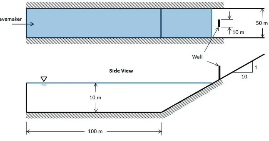
To demonstrate the method outlined above, a hypothetical scenario is postulated. A simple structure (a wall) is located on a planar beach shoreline (Figure 1). The slope of the beach face is 0.1 (i.e., 1:10), and the design incident wave condition has been determined to be a 2 meter wave height with a 12 second period. For the purposes of this example, waves will be considered as monochromatic waves, though the method could also be applied with spectral wave conditions.
Empirical Equations
the value based on Hughes (2004). This is consistent with the conservative nature of the Mase (1989) equation that has been well documented (e.g., Barcharth and Hughes [2002]).
Figure 1: Schematic of Shoreline Geometry
Simple Numerical Model
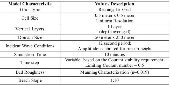
A simple numerical model was developed to characterize the beach profile (a slope of 1:10; Figure 1) without the effects of the wall. The SWASH model (Zijlema et al., 2011) was used to perform hydrostatic NLSW equation calculations for this simple scenario. The model and grid characteristics are summarized in Table 1.
In SWASH, the appropriate grid resolution for a particular modelling application depends on the wave length of the waves under consideration. For moderate or large wave heights, the SWASH manual recommends that a good model should include approximately 100 grid cells per wave length of the shortest wave length to be simulated (SWASH, 2014). For the purposes of this analysis, a 12 second wave is applied in 10 meter deep water, corresponding to a wave length of approximately 110 meters. Thus, a grid resolution of 0.5 m by 0.5 m is higher than necessary based on the SWASH manual. This higher resolution was desirable for this analysis to increase the detail of the inundation results (see validation study below).
Another modelling consideration was the roughness coefficient for the sea bottom. A Manning’s roughness coefficient of 0.019 was applied, which is a typical value for nearshore wave modelling (SWASH, 2014).
The time step for these simulations was controlled by a limiting Courant number of 0.5, which is appropriate for wind-wave modelling (SWASH, 2014).
Table 1: SWASH Model Characteristics
Model Characteristic Value / Description
Grid Type Rectangular Grid
Cell Size 0.5 meter x 0.5 meter
Uniform Resolution
Vertical Layers 1 Layer
(depth averaged)
Domain Size 50 meter x 250 meter
Incident Wave Conditions 12 second period;
Amplitude: calibrated for run-up height
Simulation Time 10 minutes
Time step Variable, based on the Courant stability requirement.
Limiting Courant number = 0.5
Bed Roughness M anning Characterization (n=0.019)
Beach Slope 1:10
Calibration
The input wave amplitude for the simplified model was calibrated to ensure that the run-up height simulated in the model was the same as the height computed by the run-up equation. Two separate calibrations were performed: one for matching the Hughes (2004) equation run-up height (1.4 m), and one for matching the Mase (1989) equation run-up height (2.0 m).
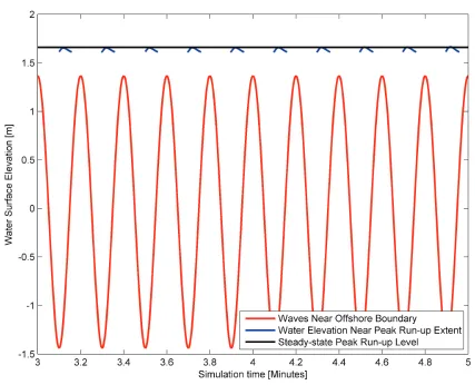
For the Hughes (2004) calibration, the initial wave amplitude for the calibration was taken as the run-up height computed from the Hughes (2004) equation (1.4 m). The run-up height in the model was measured at a point near the maximum run-up extent (Figure 2), which indicated a run-up height of approximately 1.7 m. Note that there are transient effects at the beginning of the simulation due to model spin-up (Figure 2). These effects are ignored when determining the run-up height.
Because the run-up height of 1.7 m is higher than the target run-up height (based on the Hughes [2004] equation) of 1.4 m, the two approaches are available to proceed. First, the input wave height to the model could be calibrated to align the simulated run-up height with the target run-up height. Alternately, the input leading to higher run-up heights could be retained with the understanding that his provides a small factor of safety in the analysis.
For practical engineering application, the higher run-up height (1.7 m) could be retained as conservative. However, since this scenario will be used (below) to validate the method against an independent model, it is not desirable to include any factor of safety at this point. Thus, the calibration approach is applied. After a couple of iterations, a calibrated incident wave height of 1.9 m was obtained. Thus, applying a wave field with an incident wave height of 1.9 m (and a period of 12 s) will produce the appropriate run-up level in a hydrostatic NLSW equation model for the beach under consideration (i.e., a planar beach with a slope of 0.10).
Figure 2: Run-up Results for Calibration Simulation
NOTE: This figure illustrates water surface elevations at two different locations: the offshore boundary of the model, and a point near the maximum run-up extent. The intermittent blue line corresponds to the intermittent run-up flows near the peak run-up extent. The black line indicates the peak run-up level.
Detailed Numerical Model
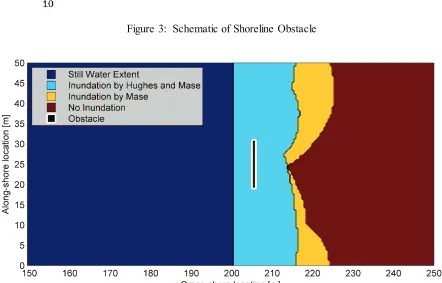
Once the model has been calibrated, the shoreline details can be added, including obstructions (and more detailed topography if applicable). In the case of this example, there is a wall (Figures 1 and 3) to be added to the model. The wall has an along-shore dimension of 10 meters and a cross-shore dimension of 1 meter. The base of the wall is located 5 meters away from the still water shoreline (at an elevation of 0.5 m above the still water level). This could correspond to a storm surge event where the still water level has increased to a relatively high level that approaches but does not actually inundate around a building. The actual inundation is only due to the presence of wind-waves.
Figure 3: Schematic of Shoreline Obstacle
Figure 4: Inundation Extents with Model Input Based on Hughes (2004) and Mase (1989)
VALIDATION
validation, the incident wave conditions for the non-hydrostatic model are the same as the conditions used for the run-up equations applied above (i.e., a 12 second period and a 2 meter wave height).
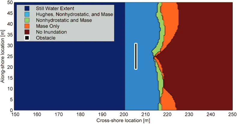
Figure 5 illustrates a comparison between the calibrated hydrostatic model results and the non-hydrostatic validation case results. Immediately behind the structure, the inundation extent based on the Mase (1989) equation provides a better comparison to the non-hydrostatic inundation extent than the inundation extent based on the Hughes (2004) equation. In areas away from the structure, the Mase (1989) characterization is conservative. The Hughes (2004) equation provides a relatively good fit for the non-hydrostatic simulation inundation extent. However, it is generally less conservative than both the non-hydrostatic and Mase (1989) inundation extents.
This variability in inundation extent is expected based on the variability indicated by different run-up equations. To within the tolerances and expected accuracy of empirical run-up equations, the inundation results shown in Figure 5 are satisfying. Figure 5 suggests that there is more variability based on the choice of empirical run-up equation than based on the modelling methodology. Consequently, application of the proposed method is appropriate, though it should be coupled with conservative run-up equations for design considerations to ensure a conservative analysis (i.e., to account for the variability in different run-up characterizations).
Figure 5: Validation by Comparison to Non-hydrostatic Model
CONCLUSIONS
This paper outlines a method for conducting numerical modelling of wave run-up inundation. The method provides a more detailed description of run-up inundation than empirical run-up equations, but operates with lower computational effort (CPU time) than more complex nearshore modelling software (e.g., Boussinesq models or non-hydrostatic non-linear shallow water equation models).
REFERENCES
Hughes, S. A. (2004). “Estimation of wave run-up on smooth, impermeable slopes using the wave momentum flux parameter,” Coastal Engineering, Elsevier, 51, 1085-1104.
Mase, H. (1989). “Random wave runup height on gentle slope,” Journal of Waterway, Port, Coastal, and Ocean Engineering, American Society of Civil Engineers, 115(5), 649-661.
Smit, P., Zijlema, M., and Stelling, G. (2013). “Depth-induced wave breaking in a non-hydrostatic, near-shore wave model,” Coastal Engineering, Elsevier, 76, 1-16.
Stockdon, H. F., Holman, R. A., Howd, P. A., and Sallenger, A. H. (2006). “Empirical parameterization of setup, swash, and runup,” Coastal Engineering, Elsevier, 53(7), 573-588.
SWASH, 2014. SWASH (Simulating WAves till Shore): User Manual, version 2.00AB, 2014.
Van der Meer, J. W. and Stam C. M. (1992). “Wave runup on smooth and rock slopes of coastal structures,” Journal of Waterway, Port, Coastal, and Ocean Engineering, American Society of Civil Engineers, 118(5), 534-550.
Van Gent, M. R. A. (2001). “Wave runup on dikes with shallow foreshores,” Journal of Waterway, Port, Coastal, and Ocean Engineering, American Society of Civil Engineers, 127(5), 254-262.
Zijlema, M. and Stelling, G. S. (2008). “Efficient computation of surf zone waves using the nonlinear shallow water equations with non-hydrostatic pressure,” Coastal Engineering, Elsevier, 55, 780-790.