Scaling up Ecosystem Services Values: Methodology, Applicability and a Case Study

Full text

(1)NOTA DI LAVORO 41.2010. Scaling up Ecosystem Services Values: Methodology, Applicability and a Case Study By Luke Brander, Institute for Environmental Studies, Amsterdam, the Netherlands Andrea Ghermandi, FEEM Onno Kuik, Institute for Environmental Studies, Amsterdam, the Netherlands Anil Markandya, BC3 Basque Centre for Climate Change, Bilbao, Spain Paulo A.L.D. Nunes, FEEM, Università Ca' Foscari di Venezia, Venice, Italy Marije Schaafsma and Alfred Wagtendonk, Institute for Environmental Studies, Amsterdam, the Netherlands.

(2) SUSTAINABLE DEVELOPMENT Series Editor: Carlo Carraro Scaling up Ecosystem Services Values: Methodology, Applicability and a Case Study By Luke Brander, Institute for Environmental Studies, Amsterdam, the Netherlands Andrea Ghermandi, FEEM Onno Kuik, Institute for Environmental Studies, Amsterdam, the Netherlands Anil Markandya, BC3 Basque Centre for Climate Change, Bilbao, Spain Paulo A.L.D. Nunes, FEEM, Università Ca' Foscari di Venezia, Venice, Italy Marije Schaafsma and Alfred Wagtendonk, Institute for Environmental Studies, Amsterdam, the Netherlands Summary The approach of using existing data on economic values of local ecosystem services for an assessment of these values at a larger geographical scale can be called “scaling up”. In a scaling-up exercise, economic values from a particular study site are transferred to another geographical setting, for instance to the regional, national or global scale. This paper proposes a methodology for scaling up ecosystem service values to a European level, assesses the availability of data for conducting this method, and illustrates the procedure with a case study on wetland values. The proposed methodology makes use of metaanalysis to produce a value function that is subsequently applied to individual European wetland sites. Site-specific, study-specific and context-specific variables are used to define a price vector that captures differences between sites and over time. The proposed method is shown to be practicable and to produce reasonably reliable aggregate value estimates. Keywords: Ecosystem Services, Value Transfer, Meta-Analysis, Wetland Values JEL Classification: C81, Q24, Q57 The authors wish to thank the European Environment Agency (EEA) for making this research possible. The researchers have also greatly benefited from discussions and cooperation with EEA staff, especially with the research coordinator Mr. Hans Vos. The usual disclaimers apply.. Address for correspondence: Luke Brander Institute for Environmental Studies De Boelelaan 1087 1081 HV Amsterdam The Netherlands E-mail: [email protected]. The opinions expressed in this paper do not necessarily reflect the position of Fondazione Eni Enrico Mattei Corso Magenta, 63, 20123 Milano (I), web site: www.feem.it, e-mail: [email protected].

(3) 1. Scaling up ecosystem services values: methodology, applicability and a case study Luke Brander 1*, Andrea Ghermandi 2, Onno Kuik 1, Anil Markandya 4, Paulo A.L.D. Nunes 2,3, Marije Schaafsma 1, Alfred Wagtendonk 1. Abstract The approach of using existing data on economic values of local ecosystem services for an assessment of these values at a larger geographical scale can be called “scaling up”. In a scaling-up exercise, economic values from a particular study site are transferred to another geographical setting, for instance to the regional, national or global scale. This paper proposes a methodology for scaling up ecosystem service values to a European level, assesses the availability of data for conducting this method, and illustrates the procedure with a case study on wetland values. The proposed methodology makes use of meta-analysis to produce a value function that is subsequently applied to individual European wetland sites. Site-specific, study-specific and context-specific variables are used to define a price vector that captures differences between sites and over time. The proposed method is shown to be practicable and to produce reasonably reliable aggregate value estimates.. Key words: ecosystem services, value transfer, meta-analysis, wetland values. JEL Classification: C81, Q24, Q57. 1. Institute for Environmental Studies, Amsterdam, the Netherlands Fondazione ENI Enrico Mattei, Milan, Italy 3 Università Ca' Foscari di Venezia, Venice, Italy 4 BC3 Basque Centre for Climate Change, Bilbao, Spain * Corresponding author: [email protected]. The authors wish to thank the European Environment Agency (EEA) for making this research possible. The researchers have also greatly benefited from discussions and cooperation with EEA staff, especially with the research coordinator Mr. Hans Vos. The usual disclaimers apply. 2.

(4) 2. 1. Introduction The approach of using existing data on economic values of local ecosystem services for an assessment of these values at a larger geographical scale can be called “scaling up”. In a scaling-up exercise, economic values from a particular study site are transferred to another geographical setting, for instance to the regional, national or global scale. Local values are thus not applied in another local context, but are used to estimate the values of all ecosystems (or ecosystem services) of similar characteristics in a larger region. Scaling up builds on the methods and tools that have been developed for value transfer, and can be seen as an extension of value transfer. Value transfer is usually applied on a case-by-case basis. The transfer of economic values of individual ecosystem services from a particular study site to another – but similar – site (the policy site) has become a common tool in ecosystem assessment. In the scaling-up exercise, economic values from a particular study site (or sites) are extrapolated to a larger geographical setting. Spatial scale is recognised as an important issue to the valuation of ecosystem services (Hein et al., 2006). The spatial scales at which ecosystem services are supplied and demanded contribute to the complexity of ecosystem valuation and management. On the supply-side, ecosystems themselves vary in spatial scale (e.g. small individual patches, large continuous areas, regional networks) and provide services at varying spatial scales. The services that ecosystems provide can be both on- and off-site. For example, a forest might provide recreational opportunities (on-site), downstream flood prevention (local off-site), and climate regulation (global off-site). On the demand-side, beneficiaries of ecosystem services also vary in terms of their locational distribution. The spatial scale over which ecosystem services are provided and received is determined by the spatial scale over which an ecosystem function has effect and the spatial scale of (potential) beneficiaries. For conceptualising the relationship between the supply and demand of ecosystem services one might imagine two overlaid maps – one representing the spatial extents of an ecosystem and the (potential) services it provides, and the other representing the spatial location of the (potential) beneficiaries of these services. It is important to recognise that ecosystem services result from the interaction of ecosystem functions and human activities. An ecosystem does not provide a service if no-one makes use of its potential to provide that service. Ecosystem services often have different groups of beneficiaries (different in terms of spatial location and socio-economic characteristics). For example, the provision of recreational opportunities by an ecosystem will generally only benefit people in the immediate vicinity, whereas the existence of a high level of biodiversity may be valued by people at a much larger spatial scale. Differences in the size and characteristics of groups of beneficiaries per ecosystem service need to be taken into account in aggregating values for each service. The management of ecosystems may be further complicated in cases where the interests of different groups of beneficiaries (possibly at different spatial scales) are in conflict. This may occur when ecosystem services are mutually exclusive (e.g. timber extraction and carbon sequestration). The values held by beneficiaries for ecosystem services may vary with a number of different factors that can be spatially defined (distance, availability of substitute and complementary sites, income, culture, and preferences). Use values are generally ex-.

(5) 3 pected to decline with distance to an ecosystem – so called distance decay. Non-use values may also decline with distance between the ecosystem and beneficiary, although this relationship may be less related to distance than to cultural or political boundaries. The availability of substitute (complementary) sites within the vicinity of a selected ecosystem is expected to reduce (increase) the value of ecosystem services from that ecosystem. Socio-economic characteristics of beneficiaries (e.g. income, culture, and preferences) are not spatial variables per se, but differences in these variables between (groups of) beneficiaries can often be usefully defined in a spatial manner (e.g. by administrative area, region or country). Consideration of the spatial scale of the provision and beneficiaries of ecosystem services is important for the calculation of the total economic value of these services (i.e. the aggregation of values across relevant areas and populations). In addition, accounting for spatial scale may be of further use in the formulation of policies to manage ecosystem services, for example in the identification of winners and losers, the need for compensation/incentives, and the design of policies such as payments for environmental services. Regarding the estimation of ecosystem service values, there are a number of important issues to be considered related to spatial scale. In discussing these scale related issues we make a distinction between the estimation of values for an individual ecosystem site and for the entire stock of an ecosystem within a large geographic area. We have referred to the latter case as „scaling up‟ ecosystem values when insufficiency of data requires applying value transfer methods. At the level of an individual ecosystem site, unit values for ecosystem services are likely to vary with the characteristics of the ecosystem site (area, integrity, and type of ecosystem), beneficiaries (number, income, preferences), and context (availability of substitute and complementary sites and services). All of these variables have a spatial dimension that can be accounted for in estimating site-specific values. For example, in terms of ecosystem area, many ecosystem service values have been observed to exhibit diminishing returns to scale (i.e. adding an additional unit of area to a large ecosystem increases the total value of ecosystem services less than an additional unit of area to a smaller ecosystem). It is therefore important to account for the size of the ecosystem being valued. For scaling up ecosystem values to estimate the total economic value of a change in the stock of ecosystems in a large geographic area, in addition to controlling for other spatial variables, it is necessary to account for the non-constancy of marginal values across the stock of an ecosystem. At the margin, a small change in ecosystem service provision (e.g. the loss of a small area) will not affect the value of services from other ecosystem sites. Non-marginal changes in ecosystem service provision, however, will affect the value of services from the remaining stock of ecosystems. As the ecosystem service becomes scarcer, its marginal and average values will tend to increase. This means that simply multiplying a constant per unit value by the total quantity of ecosystem service provision is likely to (substantially) underestimate the total value of a negative change. Appropriate adjustments to marginal values to account for large-scale changes in ecosystem service provision need to be made..

(6) 4 This paper discusses methods for scaling up existing estimates of ecosystem services‟ values to larger geographical scales (e.g., the European scale), and illustrates the metaanalytical value transfer method with a case study. Section 2 surveys the literature on value transfer methods as important building blocks for scaling-up applications. Section 3 discusses the practicability of methods for large-scale scaling up exercises. Section 4 illustrates the meta-analytical value transfer method by a case study on the valuation of European wetlands. Section 5 concludes.. 2. Methods for value transfer Value transfer is the procedure of estimating the value of an ecosystem (or goods and services from an ecosystem) by borrowing an existing valuation estimate for a similar ecosystem. The ecosystem of current policy interest is often called the “policy site” and the ecosystem from which the value estimate is borrowed is called the “study site”. This procedure is often termed benefit transfer but since the values being transferred may also be estimates of costs or damages, the term value transfer is arguably more appropriate. The use of value transfer to provide information for decision making has a number of advantages over conducting primary research to estimate ecosystem values. From a practical point of view it is generally less expensive and time consuming than conducting primary research. Value transfer can also be applied on a scale that would be unfeasible for primary research in terms of valuing large numbers of sites across multiple countries. Value transfer also has the methodological attraction of providing consistency in the estimation of values across policy sites. Value transfer methods can be divided into four categories: 1.. Unit value transfer;. 2.. Adjusted unit value transfer;. 3.. Value function transfer; and. 4.. Meta-analytic function transfer.. Unit value transfer involves estimating the value of an environmental good or service at a policy site by multiplying a mean unit value estimated at a study site by the quantity of that good or service at the policy site. Units values are generally either expressed as values per household or as values per unit of area. In the former case, aggregation of values is over the relevant population that hold values for the ecosystem in question. In the latter case, aggregation of values is over the area of the ecosystem. Adjusted unit transfer involves making simple adjustments to the transferred unit values to reflect differences in site characteristics. The most common adjustments are for differences in income between study and policy sites and for differences in price levels over time or between sites..

(7) 5. Value or demand function transfer methods use functions estimated through valuation applications (travel cost, hedonic pricing, contingent valuation, or choice modelling) for a study site together with information on parameter values for the policy site to transfer values. Parameter values of the policy site are plugged into the value function to calculate a transferred value that better reflects the characteristics of the policy site. Meta-analytic function transfer uses a value function estimated from multiple study results together with information on parameter values for the policy site to estimate values. The value function therefore does not come from a single study but from a collection of studies. This allows the value function to include greater variation in both site characteristics (e.g. socio-economic and physical attributes) and study characteristics (e.g. valuation method) that cannot be generated from a single primary valuation study. Rosenberger and Phipps (2007) identify the important assumptions underlying the use of meta-analytic value functions for value transfer: 1. There exists an underlying meta-valuation function that relates estimated values of a resource to site and study characteristics. Primary valuation studies provide point estimates on this underlying function that can subsequently be used in metaanalysis to estimate it; 2. Differences between sites can be captured through a price vector; 3. Values are stable over time, or vary in a systematic way; and 4. The sampled primary valuation studies provide “correct” estimates of resource value. 2.1 Markets for ecosystem services and distance decay effects The distance between a person and an environmental good can be an important explanatory variable of this person‟s willingness to pay (WTP) for that good. Transferring average WTP values from a study site where the relevant population is located close to the site to a policy site where the population lives much further away is likely to lead to overestimation of total WTP. Since the distribution of the population is likely to differ between the policy and study site, average distances between individuals and both sites are different, and value transfer studies should account for these differences. Based on economic theory, the effect of distance on WTP is expected to be negative, indicating a distance-decay effect. Distance-decay (DD) implies that the WTP for a certain site decreases as the distance from the agent to the site increases. In other words, use values are expected to be decreasing with distance, because the cost of visiting a site increases with every kilometre one has to travel. The higher the distance, the higher are the costs, the lower the demand3. One of the main reasons to in-. 3. Other tourism studies state that a longer journey does not necessarily create extra costs, as the trip itself can be enjoyed. Furthermore, a large distance is sometimes considered to be a positive character-.

(8) 6. clude this distance-decay effect is to determine the size of the geographical boundaries (market size) of the environmental good in question. This relevant market is the population over which the willingness to pay (WTP) values can be aggregated to calculate the good‟s Total Economic Value. Besides direct use values, non-use values are an important component of the Total Economic Value of any environmental good. The importance of distance for reliable value transfer or aggregation therefore depends on the type of value that a study site generates. There is no reason within standard economic theory why non-use values would also decrease with distance. The spatial discounting literature states that values that relate to what economists call non-use values (such as intrinsic and future values) should have much lower discount rates than use values (such as recreational, subsistence, therapeutic and aesthetic values) (Brown et al., 2002). The extent to which distance is important for reliable value transfer therefore also depends on the type of values generated by the study and policy sites. Other cases in which a distance-decay effect is less likely to occur are for goods that have importance on a large scale. In this case the distance decay effects are likely to be very small or negligible, meaning that even very far from the site, people are willing to pay. The fact that something is either of national importance, of symbolic meaning or has the status of national park implies that (a) there are likely to be fewer substitutes leading to a protection status, or (b) that knowledge about the site is widely spread. Loomis (1996, 2000) find a low DD-effect for salmon, a symbolic species, and Pate and Loomis (1997) do not find any DD-effect at all for a National Park. On the other hand, whenever goods have a local importance due to some cultural association with the good, willingness to pay is likely to fall beyond that political or social border. Examples are distance-decay effects found for “local” goods, suggested to be due to a “sense of ownership” (Bateman et al., 2004) or “spatial identity” (Hanley et al., 2003). For non-unique sites, such as a lake in a lake district, the availability of substitutes increases with distance, lowering the WTP for one particular site. As the distance to a site increases, the number of available substitutes is likely to increase as well – especially for local goods. However, substitution effects alone cannot always entirely explain DD-effects. Distance can be specified in many different ways and for reliable transfer or aggregation, the specification should be consistent. Approaches differ in (a) objective versus perceptual or subjective distance; and (b) a straight line (as the crow flies) or based on the road net/travel distance, using more sophisticated GIS applications. Travel cost studies typically use GIS based distance calculations, assuming that people minimize their costs by choosing the shortest route. However, for non-use values, which form a large share of many environmental goods (Oglethorpe and Miliadou, istic of a destination, as travellers associate a far away location with relaxation and „being away far from busy day to day life‟ or a more adventurous trip..

(9) 7. 2000; Kniivilä 2005), the least cost travel route does not matter and other specifications might be reliable. Another issue is to which part of the asset the distance should be measured. Ideally, the distance from individual A to the nearest access point of a site should be used for use-values. However, the larger the study area, the more difficult it becomes to determine the distance. 2.2 Substitute and complementary sites One of the most important contextual factors in a value transfer exercise is the availability of substitutes. Ignoring substitutes means that if the transfer is performed between a landscape poor in ecosystem services to a landscape rich in ecosystem services WTP values are likely to be overestimated (Bateman et al., 1999). The question is what happens to the WTP for good A if the quality in a comparable good B increases. A substitution effect in economics is usually defined as the increase of demand for good A when the price of good B increases. The consequence of disregarding substitutes is generally an overestimation of WTP, as the sum of the value of goods measured individually is higher than the value measured for all goods at once. For instance, respondents in an area with several lakes whose water quality is polluted will value cleaning up the first lake more than cleaning up the second lake, because (1) the first lake can be a substitute for the second lake, and (2) the respondent has a budget limitation which reduces the money available for cleaning up the second lake. Valuing goods separately and then adding up the values will overstate the true value, as every respondent will treat the ecosystem under study as if it were the first good. Disregarding complementary sites causes underestimation of WTP. Complementarity occurs when goods are consumed jointly, for instance when two sites are visited during the same trip, or when there are synergy-effects in production, for instance when quality increases at one site automatically increase the quality of another site due to dependent ecosystems. The WTP of one site is therefore likely to be dependent on other available alternatives and their characteristics. As distance from the site or the geographical scale of the study increases, the number of substitutes is likely to increase. In the economic geography literature, the spatial distribution of goods over the study area is addressed by including an indicator of accessibility. Fotheringham (1988) argues that if the WTP of both sites is dependent on distance, the substitution effect will be dependent on the relative distance between the sites. Just including distance from the agent to the substitutes therefore does not account for the proximity of substitutes, the spatial structure, and will lead to biased WTP estimates. However, no clear examples of environmental valuation studies account for such spatial structure. Another important factor in a value transfer study is to determine the relevant substitutes for a certain environmental good. Different criteria have been used to determine the relevant alternatives: All available similar ecosystems in the study area or within a certain range; or.

(10) 8. All similar ecosystems known or visited by the respondent; or All nature sites in the study area; or even All possible recreation areas (not necessarily nature based). 2.3 Aggregation of values Reliable value transfer should account for differences in socio-economic factors between the study site and the policy site. Large transfer errors can be introduced when value transfer from one region to another does not take into account the variations in relevant-socio-economic characteristics, such as income and demographics. Aggregation implies the estimation of the total WTP of a population by applying the individual WTP value-function from a representative sample to the entire population. As was first demonstrated by Smith (1975) and adopted later on by Loomis (2000), including distance in the WTP function that is used for aggregation can make an enormous difference in the total benefits estimate. The main question is what the size of the market is – i.e. to identify the population to which WTP should be aggregated and the spatial area in which this population lives. The DD effect can determine at what distance from a site people are no longer willing to pay anything for the ecosystem service in question. A very illustrative example can be found in Bateman et al. (2006), who compare different aggregation methods and assess the effect of neglecting distance-effects. Since they found that response and WTP in principle were both negatively related to distance, they also account for this location effect, besides the socio-economic factors. Instead of aggregating sample means, they apply a spatially sensitive valuation function that takes into account the distance to the site and the socio-economic characteristics of the population in the calculation of values. Thereby, the variability of values across the entire economic market area is better represented in the total WTP. They found that not accounting for distance in the aggregation procedure can lead to overestimations of total benefits of up to 600%. This study shows that reliable aggregation should be based on information about socio-economic characteristics of the most spatially disaggregated level available and should account for distance-effects. Aggregation sometimes refers to adding up the separately measured WTP values for different sites of a specific type of ecosystem to a Total Economic Value for all those sites together. However, as explained in the previous section, when these study sites function as substitutes or complements, summing up values without considering these interaction effects can lead to large aggregation biases. Aggregation can also refer to summing up the WTP for different ecosystem services of the same good. This approach may lead to double counting. As long as the functions are entirely independent adding up the values is possible. However, ecosystem functions can be mutually exclusive, interacting or integral (Turner et al., 2004). The excludability or interaction of ecosystem functions and values can also be dependent on their relative geographical position, for instance with substitutes that are spatially dependent..

(11) 9. 2.4 Geographic Information Systems Geographic information systems can be used to help link valuation data with information on the physical (ecosystem size, availability of substitute sites etc.) and socio-economic (income, population, education) characteristics of the policy site. Reliable value transfer has to account for differences in contextual factors that explain willingness to pay (WTP) for the study and policy site. There are two different sets of spatial attribute to be addressed in economic valuation of any environmental change: (a) the spatial pattern of the social, demographic and psychological characteristics of the affected population and (b) the physical characteristics of the goods and services under valuation. Ignoring the spatial aspects of the latter is assuming that they are randomly distributed over space in terms of quantity and quality. Assuming that population preferences are randomly distributed over space ignores demographic, socio-economic and cultural differences between regions, or the influence of location and distance on environmental values. The distribution will influence the substitution effects between ecosystem sites and determine interaction effects between ecosystem services, which affect aggregation possibilities. 2.5 Transfer Errors For a number of reasons the application of any of the value transfer methods described above may result is significant transfer errors, i.e. that transferred values may differ significantly from the actual value of the ecosystem under consideration. There are three general sources of error in the values estimated using value transfer: 1. Errors associated with estimating the original measures of value at the study site(s). Measurement error in primary valuation estimates may result from weak methodologies, unreliable data, analyst errors, and the whole gamut of biases and inaccuracies associated with valuation methods. 2. Errors arising from the transfer of study site values to the policy site. So-called generalisation error occurs when values for study sites are transferred to policy sites that are different without fully accounting for those differences. Such differences may be in terms of population characteristics (income, culture, demographics, education etc.) or environmental/physical characteristics (quantity and/or quality of the good or service, availability of substitutes, accessibility etc.). This source of error is inversely related to the correspondence of characteristics of the.

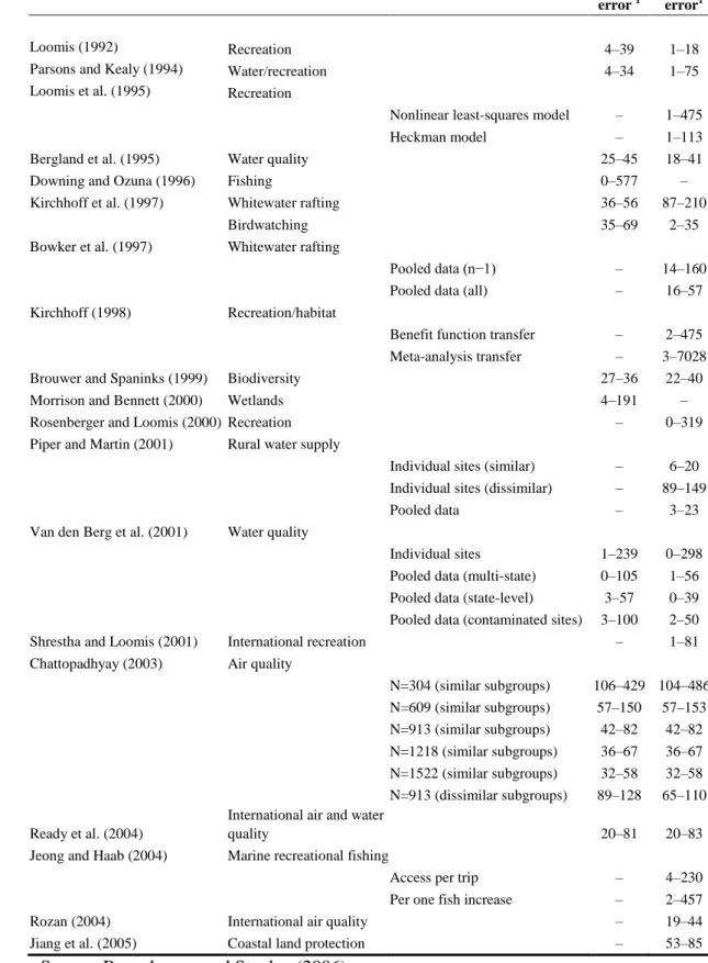
(12) 10. study and policy sites.4 There may also be a temporal source of generalisation error in that preferences and values for ecosystem services may not remain constant over time. Using value transfer to estimate values for ecosystem services under future policy scenarios may therefore entail a degree of uncertainty regarding whether future generations hold the same preferences as current or past generations. 3. Publication selection bias may result in an unrepresentative stock of knowledge on ecosystem values. Publication selection bias arises when the publication process through which valuation results are disseminated results in an available stock of knowledge that is skewed to certain types of results and that does not meet the information needs of value transfer practitioners. In the economics literature there is generally an editorial preference to publish statistically significant results and novel valuation applications rather than replications, which may result in publication bias. Given the potential errors in applying value transfer, it is useful to examine the scale of these errors in order to inform decisions related to the use of value transfer. In making decisions based on transferred values or in choosing between commissioning a value transfer application or a primary valuation study, policy makers need to know the potential errors involved. In response to this need there is now a sizeable literature that tests the accuracy of value transfer. Rosenberger and Stanley (2006) and Eshet et al. (2007) provide useful overviews of this literature. Transfer errors are generally expressed as the Mean Absolute Percentage Error (MAPE), which is defined as the difference between observed value and predicted value divided by the observed value. Table 2.1 summarises the results of a number of studies that measure transfer errors related to ecosystem values. The transfer errors presented in the table show an extremely large range from 0-7028 %. Although some studies find very high transfer errors (e.g. Downing and Ozuna, 1996; Kirchhoff, 1998) most studies find transfer errors in the range of 0-100%. Very high transfer errors may arise when the study and policy sites are very different or when the primary value to which the transferred value is compared is itself an outlier. It should be noted that the measurement of transfer errors is itself inexact in that it involves a comparison between transferred values and primary valuation estimates, 4. In the context of meta-analytic function transfer, generalisation error can arise due to the common limitation of meta-analyses to capture differences in the quality and quantity of the services under consideration. It is often the case that the provision of goods and services is indicated in a meta-analysis merely with binary variables, and that quality is not captured at all. This limitation may translate into transfer errors, as the estimated transfer function cannot reflect important quality and quantity differences in characteristics across sites. A similar problem arises where non-identical services have been combined as one explanatory variable in the meta-analysis. Some level of aggregation across service types is often necessary in order to produce a manageable number of variables in the meta-regression, but at the cost of losing specific categories of services..

(13) 11. which are subject to inaccuracies and methodological flaws of their own. In general, primary values are treated as „true‟ value observations and transferred values as approximations, whereas they are in fact both approximations. It should also be noted that a single prescribed acceptable level of transfer error is not meaningful because the level of error that is acceptable is likely to be context specific and related to other policy criteria. There are a number of studies that specifically examine the transferability of value estimates between regions and countries. We summarize some to the main findings of each study below. Loomis et al. (2005) examine the equivalency of contingent valuation (CV) results for forest fire prevention from studies in California, Florida, and Montana. They test the equality of variable coefficients across States using likelihood ratio tests. Over all tests they find mixed evidence for transferability. Brouwer and Bateman (2005) transfer contingent valuation WTP estimates for reducing health risks associated with solar UV exposure between four countries (England, Scotland, Portugal, and New Zealand) to examine the sensitivity of transfer errors to differences in contexts. When contexts are similar, mean unit value transfers are actually found to perform better than value function transfer (e.g. when transfers are between England, Scotland, and New Zealand). When study and policy site contexts are different, however, and these differences can be controlled for, value function transfer is shown to produce lower transfer errors. Kristofersson and Navrud (2007) use identical CV studies conducted in three countries (Norway, Sweden, and Iceland) to examine the validity of value transfers between those countries. The case study estimates use and non-use values for freshwater fish stocks. Values are transferred between study sites using both unit transfer and value function transfer. Equivalency analysis is applied to test the validity of value transfers. The study shows that the accuracy of value transfer relies heavily on the similarity of study sites. Eshet et al. (2007) examine the accuracy of transferring values for the disamenity of housing locations close to waste transfer stations between four cities in Israel. Value functions derived from separate hedonic pricing studies are used to transfer values for each site. Transfer errors are observed to increase with dissimilarity between sites although errors remain relatively low (2-46%). In comparing the transfer functions estimated for separate study sites, the results of Chow and Wald tests did not indicate equality between value functions and estimated coefficients. The results of the value transfers using these functions did, nevertheless, result in very low transfer errors (particularly where site characteristics were highly similar). The authors therefore argue that a finding of statistical inequality between value functions does not necessarily robustly invalidate transfers of value between sites. In other words, even though valuation studies at different sites may produce different value functions, using these functions to transfer values across sites can still result in low transfer errors..

(14) 12. Table 2.1: Summary of studies measuring value transfer errors Reference. Resource/activity. Loomis (1992) Parsons and Kealy (1994) Loomis et al. (1995). Recreation Water/recreation Recreation. Method. Nonlinear least-squares model Heckman model Bergland et al. (1995) Downing and Ozuna (1996) Kirchhoff et al. (1997) Bowker et al. (1997). Water quality Fishing Whitewater rafting Birdwatching Whitewater rafting Pooled data (n−1) Pooled data (all). Kirchhoff (1998). Biodiversity Wetlands Recreation Rural water supply Individual sites (similar) Individual sites (dissimilar) Pooled data. Van den Berg et al. (2001). International recreation Air quality N=304 (similar subgroups) N=609 (similar subgroups) N=913 (similar subgroups) N=1218 (similar subgroups) N=1522 (similar subgroups) N=913 (dissimilar subgroups). Ready et al. (2004) Jeong and Haab (2004). International air and water quality Marine recreational fishing Access per trip Per one fish increase. Rozan (2004) Jiang et al. (2005). International air quality Coastal land protection. Source: Rosenberger and Stanley (2006) 1. 1–18 1–75. – – 25–45 0–577 36–56 35–69. 1–475 1–113 18–41 – 87–210 2–35. – –. 14–160 16–57. – – 27–36 4–191 –. 2–475 3–7028 22–40 – 0–319. – – –. 6–20 89–149 3–23. 1–239 0–105 3–57 3–100 –. 0–298 1–56 0–39 2–50 1–81. Water quality Individual sites Pooled data (multi-state) Pooled data (state-level) Pooled data (contaminated sites). Shrestha and Loomis (2001) Chattopadhyay (2003). 4–39 4–34. Recreation/habitat Benefit function transfer Meta-analysis transfer. Brouwer and Spaninks (1999) Morrison and Bennett (2000) Rosenberger and Loomis (2000) Piper and Martin (2001). Unit Function transfer transfer error 1 error1. The transfer errors are the mean absolute percentage error (MAPE). 106–429 104–486 57–150 57–153 42–82 42–82 36–67 36–67 32–58 32–58 89–128 65–110 20–81. 20–83. – – – –. 4–230 2–457 19–44 53–85.

(15) 13. Ready et al. (2004) analyse the transfer of contingent valuation WTP estimates for ill health avoidance for five European countries (Portugal, Spain, England, Norway, and the Netherlands). They explore transferring values using unit value transfer, adjusted unit transfer, and value function transfer and find similar transfer errors for all three methods (20-83%). The adjusted unit transfer involved adapting estimated WTP values using the ratio of average real income in the study and policy countries. The authors conclude that a single common value function for the countries included in the study does not exist (i.e. estimated coefficients in the value functions are not the same across countries). Muthke and Holm-Mueller (2004) test the transferability of contingent valuation estimates for water quality for two German and two Norwegian lakes, thereby testing both national and international transferability. They examine unit value transfer, adjusted unit transfer, and value function transfer using the equivalence testing approach proposed by Kristofersson and Navrud (2005). They also perform Wald tests for equality of parameters. The study results show very high transfer errors for international value transfer suggesting that there was insufficient information available to fully adjust the study site values to the policy sites in another country. The authors argue that because economic factors, intrinsic values, tastes, and preferences of different cultures and societies show considerable variation, international unit value transfer is not feasible and that adjusted unit value transfer and value function transfer are also limited in the account they can take of differences in determining factors. The existing evidence on regional and international value transfer suggests that there are significant differences between regions in the determinants of environmental values that are not being adequately controlled for in value transfer exercises. The results show that as study and policy sites become more different, transfer errors tend to increase. Regarding the accuracy of meta-analytic value transfers there is more limited evidence. Rosenberger and Phipps (2001) compare transfer errors between demand function estimates and meta-analytic function estimates using travel cost data for hiking trips in Colorado. The meta-analytic function transfers are shown to result in lower transfer errors. Engel (2002) also specifically compares the performance of benefit function transfers and meta-analysis based function transfers. The results of this comparison are mixed but the conclusions produce an encouraging view of metaanalysis based transfers. Eshet et al. (2007) describe their analysis as a “mini meta-analysis function transfer” because they use data and transfer functions from four separate samples and locations (including combinations of data from multiple sites). Their analysis is not, however, a meta-analysis in the sense that results from multiple samples and study sites are examined in a regression analysis. Lindhjem and Navrud (2007) conduct a meta-analysis of contingent valuation results for non-timber forest benefits from Norway, Sweden, and Finland. They examine the accuracy of using alternative specifications of the meta-analytic value function to predict the value of selected observations in their dataset. The best model (a.

(16) 14. restricted double-log model) produces mean and median transfer errors of 47% and 37% respectively. This transfer error is lower than that resulting from simple mean unit value transfer from studies from the same country (86%, 41%), and considerably lower than when the mean unit value transfer includes the results of studies from other countries (166%, 85%). These results provide some positive support for metaanalytic value transfer but also illustrate the differences in values between countries, even those with very similar economic, social, and institutional characteristics. Brander and Florax (2006) use a meta-analytic value transfer function to estimate values for wetlands in the San Joaquin Valley (SJV) in California and for the Norfolk Broads in the UK. The lowest transfer error observed in this exercise is 29% for the valuation of water quality/nutrient retention, recreational hunting and fishing, other recreational activities and amenities in the SJV. Transfer errors of just over 50% are made for recreational hunting in the SJV, and for biodiversity and landscape maintenance and recreational activities in the Norfolk Broads. The transferred value for bird watching in the SJV, however, is over five times the primary value for this activity. Using a database of wetland values, Brander et al. (2006) employ an n–1 data splitting technique to estimate 200 meta-analytic value transfer functions and then test the accuracy of each function for predicting the value of the omitted observation in each case. The overall average transfer error is 74% with slightly less than 20% of the sample having transfer errors of 10% or less, and roughly 15% of observations showing transfer errors over 100%. Brander et al. (2007) perform a similar analysis using a database of coral reef recreation values. In this case the average transfer error for the sample of 73 value observations is 186%. The results of the above described studies that examine transfer errors resulting from meta-analytic function transfer are summarised in Table 2.2. Table 2.2: Summary of studies measuring meta-analytic function transfer errors Reference. Resource/activity. Lindhjem and Navrud, 2007. Non-timber forest benefits Restricted double-log model Full double-log model. Brander and Florax, 2006. Method. Wetland, multiple services Wetland, bird watching Wetland, hunting Wetland, biodiversity Wetland, recreation Wetland, non-use Brander et al, 2006 Wetland, multiple services Brander et al, 2007 Coral reef, recreation 1 The transfer errors are the mean absolute percentage error (MAPE). Meta-analytic function transfer error 1 47% 29% 433% 52% 53% 59% 99% 74% 186%.

(17) 15. 3. Practicability of methods, data requirements, and data availability 3.1 Practicability of methods The aim of this assessment of value transfer methodologies is to identify a practical procedure for scaling up estimates of ecosystem service values to the European level. Such a procedure should be feasible given the availability of existing data on ecosystem service values and ecosystem characteristics. Navrud (2007) develops a practical approach for value transfer in the context of Danish environmental planning. The proposed approach is adjusted unit value transfer using estimated values per household or individual. Values are aggregated over the affected population at the policy site. This methodology is practical and straightforward for transferring values to specific policy sites but may be less suitable for large scale value transfers, for example in valuing all ecosystems at a regional, national, or European scale. First, this method relies on the identification of ecosystem valuation studies that correspond most closely with the policy site under consideration. This process could become burdensome as the number of policy sites increases. Second, transferring values per household or individual requires an assessment of the relevant affected population for each ecosystem, which again could become laborious with a large number of policy sites. Transferring values in per household/individual terms may also be problematic for ecosystem services that are generally not valued in these terms. Indirect use values, such as water filtration, are more likely to be valued as inputs in production (e.g. using production function or net factor income valuation methods) and are not expressed in per household terms. Meta-analytic function transfer on the other hand is well suited to valuing large numbers of diverse policy sites in that the estimated value function can be applied to a database containing information on ecosystem and socio-economic characteristics of each site. It is a simple operation to “plug in” the characteristics of each policy site into a value function to estimate its value. If the value function is defined in terms of values per unit of area it is also a simple operation to aggregate values over spatial areas. Although this approach does not involve aggregation over the affected population, differences in „market size‟ can still be taken into account through the inclusion of population in the vicinity of the ecosystem as an explanatory variable in the value function. A clear limitation of meta-analytic function value transfer is related to the reliability of the estimated values. Evidence from the economic valuation literature shows that there are potentially very large transfer errors associated with this approach and that in some cases the relatively simple transfer of unit values may perform at least as well (see previous chapter). It is therefore advisable to test the transfer accuracy of a meta-analytic function in order to provide information about the reliability of the results..

(18) 16. A further potential drawback of using meta-analytic function value transfer is that it is likely to result in varying unit values across European regions. Due to differences in income levels and population densities across Europe, estimated ecosystem values per unit of area are likely to vary between regions. While this makes sense from an economic point of view, it may be politically sensitive, particularly if such information is used to make decisions regarding the allocation of conservation resources. 3.2 Data requirements On balance, meta-analytic function value transfer offers the most practical approach to scaling up ecosystem service values to a European scale.5 The development of such functions requires sufficient data on the value of ecosystem services. Furthermore, the application of this value transfer approach requires sufficient data on the physical, spatial, and socio-economic characteristics of each ecosystem site under consideration. A value transfer function is used to estimate a site specific „per hectare‟ value based on the ecosystem site‟s characteristics, such as size, type, abundance, and on the characteristics of the population that has a demand for the services of that site. In general form, a meta-analytic value function can be written as: yi. a bS X Si. bE X E i. bC X Ci. The variable yi measures the value of ecosystem site i, based on three vectors of explanatory variables, namely characteristics of (i) the valuation study XS, (ii) the valued ecosystem XE,, and (iii) the socio-economic and geographical context XC. The coefficients bs, bE and bc are the vectors containing the coefficients of the explanatory variables, and a is a constant. In order to estimate this function and to use it for value transfer, we need: 1.. Data on actual values of {y,X} for a sufficient number of ecosystem study sites (original valuation studies). With these data, a meta-analytical regression model is built to estimate the coefficients a and b. An example of such a meta-analytical regression model for wetland ecosystems is presented in the next chapter of this report.. 2.. Data on {XE ,XC} for all policy sites within the relevant area (e.g., Europe). The value transfer is done by plugging in these policy site data in the metaanalytical regression model.. The vector XE includes ecosystem characteristics such as area and type. In our methodology we use hectares as the unit of area. For the ecosystem categorisation we propose to use the same ecosystem types as used in the EEA land cover data. These are given in Table 3.1. Differences between wetland sites in terms of the provision of. 5. A brief discussion of alternative approaches and how these could be robustly compared with meta-analytic function transfer in future work is provided in section 5..

(19) 17. ecosystem services may be included in the XE vector, either as dummies (yes/no) or as continuous variables. The vector XC includes socio-economic and geographical context variables such as income per capita of the population around the site, population density around the site, and some measure of ecosystem abundance at the local or regional level. Other variables that determine the population‟s demand for the ecosystem services could be included as well, depending on what the meta-analytical regression identified as significant explanatory variables. Table 3.1: Ecosystem types used in EEA land cover data Code. Ecosystem type. Code. Ecosystem type. 3.1.1 3.1.2 3.1.3 3.2.1 3.2.2 3.2.3 3.2.4 3.3.1. Broad-leaved forest Coniferous forest Mixed forest Natural grassland Moors and heathland Sclerophyllous vegetation Transitional woodland shrub Beaches, dunes and sand plains Bare rock Sparsely vegetated areas Burnt areas Glaciers and perpetual snow. 4.1.1 4.1.2 4.2.1 4.2.2 4.2.3 5.1.1 5.1.2 5.2.1. Inland marshes Peatbogs Salt marshes Salines Intertidal mudflats Water courses Water bodies Coastal lagoons. 5.2.2. Estuaries. 3.3.2 3.3.3 3.3.4 3.3.5. The availability of the two types of data (study sites and policy sites) is discussed in the following sections. 3.3 Data availability Availability of ecosystem service value data Several good databases of environmental valuation results are available. The most comprehensive database is the Environmental Valuation Reference Inventory (available at the EVRI web-page http://www.evri.ec.gc.ca/evri/). Other useful online resources are Envalue (http://www.environment.nsw.gov.au/envalue/), the Ecosystem Services Database (http://esd.uvm.edu/). A number of country specific valuation databases have also been developed, such as the Environmental Valuation Source List for the UK (www.defra.gov.uk/environment/evslist/index.htm) and ValueBase for Sweden (http://www.beijer.kva.se/valuebase.htm). In addition, a number of ecosystem specific value databases have been constructed (e.g. for European forest valuation studies under the E45 Cost Action on European Forest Externalities project). These databases provide good starting points for the collection of economic valuation studies for the purposes of value transfer. The data usually comprises bibliographic.

(20) 18. information and summaries of methods and results. Conducting meta-analyses using this information requires the construction of numerical databases specifically for this purpose. Several meta-analyses have been conducted in the field of economic valuation of environmental resources, impacts, and services. Table 3.2 below lists a number of meta-analyses of ecosystem values. Table 3.2: Meta-analyses of ecosystem values Ecosystem/ecosystem service. Meta-analysis study. Wetlands. Brouwer et al., 1999 Woodward and Wui, 2001 Brander et al., 2006 Ghermandi et al., 2007 Boyle et al., 1994 Brander et al., 2007 Bateman and Jones, 2003 Lindhjem, 2007 Smith and Karou, 1990 Rosenberger and Loomis, 2000 Shrestha and Loomis, 2001 Nijkamp et al., 2008 Jacobsen and Hanley, 2007 Loomis and White, 1996 Kaoru and Smith, 1995 Barton, 1999 Brander and Koetse, 2007. Groundwater Coral reef recreation Woodland recreation Non-timber forest benefits Outdoor recreation. Biodiversity Endangered species Urban air pollution Marine and coastal water quality Urban open space. A comparison with Table 3.1 suggests that with respect to “type”, there is no complete mapping between study sites and policy sites. Additional research is needed to identify the most important “gaps”, and to examine whether additional meta-analyses could be carried out on the basis of existing original valuation studies. For some important ecosystems, such as wetlands and forests, meta-analyses of ecosystem values do exist and these could be used directly for the purpose of value transfer. Spatial variables for meta-analytic value transfer As discussed above, meta-analytic value functions are likely to include a number of variables that have a spatial dimension, including ecosystem size, ecosystem abundance, population within a given proximity of an ecosystem, and income per capita of that population. Table 3.3 presents data sources that could be used to construct these spatial variables on a European scale..

(21) 19. It should be noted that the proposed value transfer process estimates values for individual ecosystem „sites‟ (distinct separate patches of a specific ecosystem type).6 In other words, ecosystem sites are the units of analysis in the value transfer exercise and therefore spatial variables need to be defined at this level. Table 3.3: Spatial data sources Data set. Download source / owner. GIS datamodel / format. Coordinate system and extent. Scale / resolution. Year. Vector polygon / ESRI Shape. Lambert Azimuthal Equal Area. 1:100 000. 2000. 2.5 arc-minute. 2000. Corine land cover 2000 (CLC2000) seamless vector database Version 10 jan 2007. EEA Dataservice. Gridded Population of the World, version 3 (GPWv3). Socioeconomic Data and Applications Center (SEDAC) operated by CIESIN http://sedac.ciesin.columbi a.edu/gpw. GRID (ESRI). Administrative land accounting units GISCO administrative boundaries (NUTS) v9. EEA Dataservice. Vector polygon / ESRI Shape. Lambert Azimuthal Equal Area Europe. 1:1 000 000. 2004. Income per capita. Eurostat table reg_e2gdp. Table. Lambert Azimuthal Equal Area Europe. NUTS level 13. 2003. http://www.eea.europa.eu/ EEA. http://www.eea.europa.eu/. Europe. WGS 1984 Europe. Gross domestic product (GDP) in 2003 at current market prices at NUTS level 2. Ecosystems The spatial data that need to be generated for ecosystem characteristics are: Locations of individual sites of each ecosystem type. Ecosystem size (in hectares) for each individual ecosystem site. 6. See section 4.5 for a full description of the proposed value transfer procedure. In brief, a value transfer function is used to estimate a site specific „per hectare‟ value based on each ecosystem site‟s characteristics (size, type, abundance, socio-economics). This „per hectare‟ value is then multiplied by the area of the site to obtain a total value for that site. The values of individual sites can then be aggregated to obtain values for each ecosystem within a region, country, or Europe as a whole..

(22) 20. Ecosystem abundance, which is defined as the total area of an ecosystem type within some radius (in km) of the centre of each ecosystem site. The degree to which a particular ecosystem type is scarce is in part determined by the scale of analysis. It is possible, for example, for a particular ecosystem type with a cluster of sites to be considered abundant at a local scale but very scarce at a European scale (if there is a small total area of this ecosystem type). The necessary steps construct in ArcGIS a geo-referenced map of ecosystem areas in Europe from the Corine land cover database are illustrated by the construction of a wetland area map (ecosystem codes 4.1.1, 4.1.2, 4.2.1, 4.2.2, and 4.2.3 from Table 3.1). Figure 3.1 presents the resulting map of European wetlands.. Figure 3.1: Map of European wetlands To determine the surface area of each ecosystem site we have used the Corine seamless vector land cover data (CLC2000). The sizes of the areas of individual ecosystem sites have been calculated with the calculate geometry function in ArcGIS. We also calculated the centerpoints of the areas of the ecosystem sites. In the map example in Figure 3.2 the calculated centerpoint locations are displayed on top of the ecosystem site areas (polygons) for the type broad-leaved forest..

(23) 21. Figure 3.2: Centerpoints (red points) of ecosystem type broad-leaved forest (Code 3.1.1) The ecosystem abundance is defined as the summed area of ecosystems within some radius of the centerpoint of each ecosystem site. In the examples used in this section, the radius is set at 50 km. This ArcGIS procedure has been modelled for a test area containing a large part of the Netherlands with ArcGIS model builder. It produces from the Corine (seamless vector) database for all sites of 21 different ecosystem types an abundance indicator value expressed in hectares. In the map example in Figure 3.3 the abundance of the ecosystem types broad-leaved forest and natural grassland are represented by the calculated background 100 meter raster map in which the highest scarcity is represented by the darkest areas..

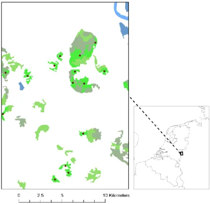
(24) 22. Upper panel: Abundance of broad-leaved forest from less abundant (black) to abundant (white) Lower panel: Abundance of natural grassland from less abundant (black) to abundant (white) Figure 3.3: Ecosystem abundance indicators for broad-leaved forest and natural grasslands in the Netherlands The map in Figure 3.4 shows an indicator of wetland abundance. It shows the centerpoint (red point) of an intertidal mudflat in Northern Ireland (ID 45970) with a.

(25) 23. surface of 805 hectares, surrounded by 147,406 hectares of other wetland areas in a circular 50 km zone.. Figure 3.4: Wetland abundance in Northern Ireland. Population The spatial data that need to be generated regarding population characteristics concern the population in the vicinity of the ecosystem site (usually defined within some radius of the centre of each ecosystem site). The process by which this data can be generated is described in Wagtendonk and Omtzigt (2003). For the population data we can choose between two available population data sets for Europe: 1. The Gridded Population of the World dataset (GPWv3) of the Socioeconomic Data and Applications Center (SEDAC). File name: euds00ag (ESRI GRID format). 2. The population density dataset of the Joint Research Centre (EC-JRC). This is a disaggregated dataset (to 100 meter gridcells) based on the Corine land cover 2000 map. A choice between these two datasets has to be made based on the required spatial resolution versus processing time needed for calculating average population densities in zones with a radius of 50 km around ecosystem sites..

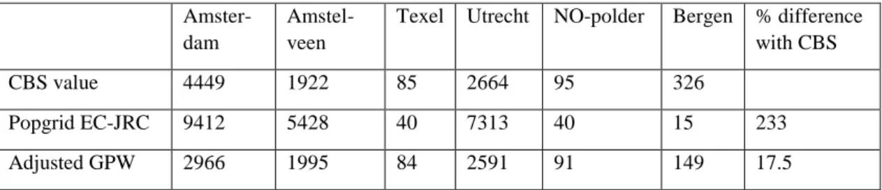
(26) 24. We have performed a simple test using spatial statistics of Statistics Netherlands (Wijk- en buurtkaart CBS 2001), containing, among others, population density figures for all municipalities in the Netherlands. The test showed that on a municipal level the population density figures of the GPW dataset shows by far the best results for the tested municipalities (respectively 17.5 % difference and 233 % difference with the CBS figures, see Table 3.4). It has to be remarked however that the 100 meter gridcell values of the EC-JRC dataset show in general better values when zoomed in to the centres of separate towns. We are however more interested in average population density figures for larger areas and have therefore chosen to use the GPW dataset. It has to be noted that this test has only been performed on Dutch population density figures and not on figures for other countries in Europe. Still we expect this test to be representative. A second reason to choose for the GPW dataset is the larger gridcell resolution of 2.5 arc-minute (circa 4.6 by 4.6 km) which will be much faster to process than the EC-JRC 100 meter gridcells. Table 3.4: Comparison of EC-JRC and GPW population density datasets with official (CBS) density figures of some Dutch municipalities Amsterdam. Amstelveen. Texel. Utrecht. NO-polder. Bergen. % difference with CBS. CBS value. 4449. 1922. 85. 2664. 95. 326. Popgrid EC-JRC. 9412. 5428. 40. 7313. 40. 15. 233. Adjusted GPW. 2966. 1995. 84. 2591. 91. 149. 17.5. As source data we used the population data provided by the International Earth Science Information Network (CIESIN), of Columbia University. Income The spatial data that need to be generated regarding economic characteristics concern income per capita of the population in the vicinity of each ecosystem site. Ideally the population to which the income data relates should be the population that hold values for the ecosystem in question. As it would be unfeasible to identify this population for each ecosystem site, we propose to use income per capita at the NUTS2 level. GIS can be used to link the location of each ecosystem site to the relevant NUTS2 region. The income figures per capita for the NUTS areas in which the ecosystem sites are located can be calculated by combining Eurostat statistics for Gross Domestic Product (GDP) in 2003 (table reg_e2gdp.xls) at current market prices at NUTS level 2 with the administrative map units downloaded from the EEA dataservice: Administrative land accounting units GISCO (NUTS) v9..

(27) 25. 4. Case study 4.1 Introduction In this section the economic value of services and goods from wetlands in the European Union is estimated based on the meta-analytic value transfer methodology and scaling up procedure introduced in the previous sections. The preliminary work carried out by Ghermandi et al. (2007), who performed a meta-analysis of a very large number of wetland valuation studies provides the starting point for the scaling up valuation procedure. A wide range of relevant explanatory variables is included in the meta-analysis and value transfer exercise, including the abundance of wetlands, the type of ecosystems services provided, the population in the vicinity of each wetland, the GDP per capita (at NUTS2 level for European observations), the size of each wetland, and the economic valuation method used. In the scaling up exercise, the meta-analytic value transfer function is combined with the spatial information on 50,533 individual wetland sites generated with a GIS from the Corine land cover. 4.2 The wetland valuation literature The monetary estimation of the market and non-market benefits of wetlands has been the subject of a large number of primary valuation studies. Since the publication of the first wetland valuation study in 1974 (Hammack and Brown, 1974), the number of studies aimed at estimating the value of wetlands has steadily grown. The most extensive review of the wetland valuation literature up to date is by Ghermandi et al. (2007) and counts 383 value observations from 166 independent valuation studies. This large number of closely related and comparable studies has stimulated the use of research synthesis techniques known as meta-analysis. Four meta-analyses of wetland valuation studies have been published: 1. Brouwer et al. (1999) analyze the results of contingent valuation method (CVM) studies of temperate climate zone wetlands. The definition of wetlands used in this study is very broad and the meta-analysis includes a number of valuation estimates for open water (rivers and lakes). The focus on estimates from CVM studies in developed countries, mainly the United States, narrows the sample size to 92 value observations from 30 studies. 2. Woodward and Wui (2001) similarly restrict the scope of their meta-analysis to include valuation studies for North American and European wetlands only. They use a narrower definition of wetland than Brouwer et al. (1999) while also including wetland values obtained with valuation techniques other than CVM. The resulting data set contains 65 value observations taken from 39 studies. 3. Brander et al. (2006) assembled a dataset of 215 value observations obtained from 80 studies. Their analysis includes studies from temperate and tropical regions, for different wetland types (including mangroves), and for a broader set of wetland functions and valuation methods. An important element of this meta-analysis is the addition of external socio-economic variables like GDP per capita and popula-.

(28) 26. tion density. In spite of the broad geographical scope adopted, the distribution of primary valuation studies is still very much biased by the practice and availability of natural resource valuation studies rather than by the distribution of wetlands. In particular, studies from North America accounted for half of the total number of observations. 4. Ghermandi et al. (2007) greatly expanded the data set used in Brander et al. (2006) to include by far the largest number of primary valuation studies used in a meta-analysis of wetland values: namely, 383 independent observations derived from 166 studies. With respect to previous meta-analyses, there is an extension of the geographical coverage of the studies, which is less biased towards developed Western countries. Indeed, a clear increase in the number of studies from Africa, Asia and Europe in recent years is identified, while the number of new studies from North America – where wetland valuation was first widely used – shows a downward trend. In addition, man-made wetlands are included for the first time in a meta-analysis of wetland values. The innovative contributions of this model include the recognition of substitution effects between wetland sites and environmental pressure as important explanatory variables of wetland values. Furthermore, the presence of human pressures on the wetlands is taken into account in the analysis by means of an index of environmental stress and is recognized to lead to higher values. 4.3 Description of the data set and the meta-regression model The data set of wetland values The data set used for the determination of the meta-analytic value transfer function relies on the work conducted by Ghermandi et al. (2007). Figure 4.1 provides an overview of the location of the valued wetland sites and the year of publication of studies examined by Ghermandi et al. (2007). Despite the focus of the case study on scaling European wetland values, the data set underlying the meta-regression analysis is not limited to European sites only. Reasons for this include the need to provide a sufficient number of observations for wetland services that are not frequently object of valuation studies (e.g. non-use values) and guarantee a sufficient degree of variability in the explanatory variables of the meta-regression. A large degree of variability in the explanatory variables is in fact not a limit to the meta-analysis as far as it can be assumed that there exists a single underlying function that links the size of a specific effect on the dependent variables to the explanatory variables. On the contrary, a sufficient degree of heterogeneity is necessary to robustly identify the size of a specific effect on the dependent variable. All continents are represented in the data set. The largest number of observations is derived from North American studies (129), but a significant fraction comes from Asia (89), Europe (78) and Africa (53). South America (18) and Australasia (16) are less well represented. The studies included in the data set are all primary valuation.

(29) 27. studies and, in order to limit the risk of introducing a publication bias, the analysis is not limited to publications from the “official scientific literature”, but also explores the complementary areas of “grey literature” (e.g. reports for both public and private institutions, consultancy studies) and unpublished research results. The average number of observations per study (2.3) and the maximum number of observations for a single study (10) is relatively low if compared to the total number of observations used in the analysis (383). As such, multiple sampling bias is expected to have a scarce influence on the results of the investigation.. Europe 40. 20 0 Year of publication. Asia 40. 20 0 Year of publication. Nr.of obs.. Nr.of obs.. Nr.of obs.. North America 40. 20 0 Year of publication. South America. 20 Africa 0. Australasia. 40. Nr.of obs.. Year of publication. 40. Nr.of obs.. Nr.of obs.. 40. 20 0 Year of publication. 20 0 Year of publication. Figure 4.1: Number of observations of wetland values in intervals of five years from 1972 to 2007 and geographical location Since the goal of the meta-regression performed in this study is to provide a metaanalytic value transfer function to be applied to the spatial information derived from the CORINE map concerning of land uses in countries in the European Union, it was not possible to make use of the whole data set of valuations. Due to the large scope of the meta-analysis performed by Ghermandi et al. (2007) in fact, the definition of wetland upon which the selection of ecosystems types and valuation studies was based is a comprehensive one. It encompasses all ecosystem types embraced by the Ramsar definition7 with the exception of rice cultivations, coral reefs, sea-grass beds,. 7. The definition of provided by the Ramsar Convention on Wetlands of International Importance identifies as wetland any area of “marsh, fen, peatland or water, whether natural or artificial, permanent or temporary, with water that is static of flowing, fresh, brackish or salt, including areas of marine water the depth of which at low tide does not exceed six meters” (art. 1.1).

(30) 28. rivers, and shallow lakes, which are implicitly included in the Ramsar definition but are seldom regarded as wetlands (Scott and Jones, 1995). The definition of wetland used in the EEA land cover data, however (see Table 3.1), is more restrictive and explicitly excludes wooded areas such as wet forests and forested floodplains, which are classified as forest ecosystems, and estuaries and coastal lagoons, which are regarded as water bodies. Furthermore, the data set by Ghermandi et al. (2007) includes a number of tropical ecosystems (e.g. mangroves), which do not naturally occur in European countries. For all the mentioned reasons, the original data set was restricted to include only ecosystems that are compatible with the definition of wetland used in the EEA land cover data. The total number of usable observations was reduced to 264. The meta-regression model and the explanatory variables The meta-analytical regression model used for the estimation of wetland values is illustrated in matrix notation, in equation 1. ln( y i ). a bS X Si. bW X Wi. bC X Ci. ui. (1). The dependent variable (y) in the meta-regression equation is the vector of the wetland values standardized to 2003 US$ per hectare per year. The subscript i assumes values from 1 to 264 (number of observations), a is the constant term, bs, bw and bc are the vectors containing the coefficients of the explanatory variables and u is the vector of residuals. Table 4.1 provides an overview of the explanatory variables. They consist of three categories, namely characteristics of (i) the valuation study XS, (ii) the valued wetland XWi and (iii) the socio-economic and geographical context XC. The variable type (nominal, interval, or ratio) is also reported. Study characteristics (XS). Study characteristics accounted for in the model include the valuation method used and a dummy distinguishing between marginal and average values (Brander et al., 2006). A wide array of valuation methods has been used in the primary studies for the assessment of the different values of wetlands. These include market-based methods – i.e., market prices (61), net factor income (34), opportunity cost (9), replacement cost (56) and production function (14) –, revealed preference methods – i.e., travel cost method (42) and hedonic pricing (5) –, and stated preference methods – i.e., contingent valuation method (62) and choice experiment (8). A dummy for each of the valuation methods is included in the meta-regression model to account for the heterogeneity of methods, as not all of them have a strong basis in welfare theory and as they produce estimates of different welfare measures. In standardizing wetland values we face the problem of distinguishing between average and marginal values, both of which can be expressed as a monetary value per hectare. To distinguish between marginal and average per hectare values in the metaregression, following Brander et al. (2006), a dummy variable is introduced, which takes a value equal to one for marginal values (36) and equal to zero for average values (228)..

(31) 29. Table 4.1: Explanatory variables used in the meta-regression model Group Study (XS). Variable Valuation method. Variable type Levels / measurement unit Nominal Contingent valuation method Hedonic pricing Travel cost method Replacement cost Net factor income Production function Market prices Opportunity cost Choice experiment Marginal / average Nominal Average Marginal Wetland Wetland type Nominal Inland marshes (Xw) Peatbogs Salt marshes Salines Intertidal mudflats Wetland size Ratio Hectares (ln) Service provided Nominal Flood control and storm buffering Surface and groundwater supply Water quality improvement Commercial fishing and hunting Recreational hunting Recreational fishing Harvesting of natural materials Fuel wood Non-consumptive recreation Amenity and aesthetics Biodiversity Context GDP per capitaa Ratio 2003 US$ person-1 year-1 (ln) (XC) Population density Ratio Inhabitants in 50 km radius in year 2000 (ln) Wetland abundance Ratio Hectares in 50 km radius (ln). 0N 062 005 042 056 034 014 061 009 008 228 036 182 021 064 000 041 264 034 033 038 053 047 049 039 013 070 034 036 264 264 264. N = number of observations for each variable or variable level a. At NUTS 2 level for European observations, state level for observations form the U.S.A., and country level for all other observations. Wetland characteristics (XW). Characteristics of the valued wetland site that are accounted for in the meta-regression model are the type and size of the wetland and the types of services provided. The wetlands in the database are classified according to the EEA land cover nomenclature for wetland ecosystems. According to the EEA classification (see Table 3.1), inland wetlands include inland marshes and peatbogs, while coastal wetlands are classified into salt marshes, salines, and intertidal mudflats. As large wetlands may include areas with very different characteristics, the same observation may be classified under two or more wetland systems. The large majority of the wetlands in the database are inland marshes (182). A significantly lower number of observations.

No results found