Performance Based Ratings for the ENERGY STAR
®Windows Program: A discussion of issues and future
possibilities
August 1, 2003
Prepared by:
Dariush Arasteh, Robin Mitchell, and Steve Selkowitz
Windows and Daylighting Group
Lawrence Berkeley National Laboratory
For:
Marc LaFrance and Richard Karney
Office of Building Technology
Energy Efficiency and Renewable Energy
U.S. Department of Energy
Background
The ENERGY STAR® Windows program sponsored by the US Department of Energy has gained widespread participation by window manufacturers throughout the United States as a means to identify and market high performance residential window, skylight, and door products1. ENERGY STAR qualifying criteria are based on the two main thermal indices typically used to quantify the energy performance of window and other fenestration products: the U-factor and the Solar Heat Gain Coefficient (SHGC)2. These properties respectively quantify heat loss (or gain) as a function of a temperature
difference and the fraction of solar energy transmitted by the window. Complete product U-factors and SHGCs are required to be calculated in accordance with the procedures developed by the National Fenestration Rating Council (NFRC), a non-profit group representing a diverse set of stakeholders in the window and building industry.
U-factors are ideal for quantifying heat flow through a window at a specific set of conditions (i.e. outdoor temperatures, indoor temperature, wind speed). Similarly,
1
Throughout this white paper, the term windows will be used to refer to all fenestration products including doors and skylights. Proposed tradeoffs are presented only for windows; ultimately, alternative tradeoffs will have to be prepared for skylights and doors separately.
2
In this paper, references to ENERGY STAR are references to the ENERGY STAR Windows criteria, effective August 29, 2003.
SHGCs capture the instantaneous solar heat gain under a specific set of conditions (sun angle, window orientation, cloud cover, etc.). However, annual energy performance is a function of both these parameters. During the heating season, U-factors quantify heat lost to the outdoors (the dominant effect) and SHGCs quantify beneficial solar gain to the space. During the cooling season, U-factors quantify heat gains/losses from/to the
exterior and SHGCs quantify heat gains from incident sunlight (the dominant effect) . (Ultimate energy use is also influenced modestly by the product’s air infiltration (AI) rate, a parameter currently not part of the ENERGY STAR program.) ENERGY STAR recognizes the importance of both U and SHGC by setting separate requirements for each parameter in each climate zone. These requirements take the form of maximum U-values for all four zones and maximum SHGCs for all but the northern zone. The northern region does not include a requirement on SHGC (either maximum or minimum) due to the dominant role of U-factor on energy use. The ENERGY STAR web site
(http://www.energystar.gov/index.cfm?c=revisions.windows_spec) provides more details on the updated ENERGY STAR program.
It is recognized by both DOE and industry that other combinations of window properties which do not strictly meet both U and SHGC prescriptive requirements for a given zone may result in levels of energy performance equivalent to products which meet the
prescriptive requirements. For example, in a southern climate, lowering the SHGC below the ENERGY STAR requirement will save additional cooling energy. If a certain
product accomplishes this but has a slightly higher U-factor (leading to increases in heating energy), its total energy use may be equivalent to that of an ENERGY STAR qualifying product.
Looking at total annual energy use based on combinations of U and SHGC as a
qualifying route to ENERGY STAR is termed “performance based” and is the subject of this white paper. Issues which would need to be addressed to develop a fair performance based approach are discussed. Several options to a performance based ENERGY STAR program are proposed and the pros and cons of each option are proposed. This white paper is not meant to be a definitive statement on the topic; it is rather a summary of the background issues and a presentation of future options, based on DOE supported work in this field for the past decade. It should be seen as the starting point for discussions in and among industry, DOE, and other interested parties.
Issues for Consideration
Issues which must be considered in the development of a performance based system for ENERGY STAR windows are presented in this section. These issues are presented in order to better understand the pros and cons of the different approaches to the
performance based systems presented in the next section. These issues are based on:
1) background research on NFRC’s efforts to develop an annual energy rating system in the 1990s.3
2) analysis effort over the past two years in support of revised ENERGY STAR criteria
3) input from manufacturers and other interested parties.
Analysis Tool
The use of simulation software to evaluate window thermal and optical properties (i.e. U-factor, Solar Heat Gain Coefficient, Visible Transmittance, etc.) has established itself as much more cost-effective and consistent than physical testing. To develop a performance based rating system, simulation software capable of modeling the annual energy impacts of windows in houses is required. Testing windows in typical homes is clearly not feasible due to the huge cost and resulting uncertainties in such testing programs.
Fortunately, tools exist which are well suited to this task. DOE2 (and its successor Energy Plus), a complete building energy analysis tool, have been developed by the US Department of Energy for evaluating total building energy use. DOE2 has been used extensively and continually updated since its early release in the 1970s. This software has been well validated against experimental data (Sullivan and Winkelmann, 1998). Relative savings between different window products have been observed to be in much better agreement than absolute energy use. While other building energy simulation codes could also be used, DOE2 is considered by many experts as the current definitive tool; it has also been used extensively within NFRC’s efforts during the past decade to develop an annual energy rating.
RESFEN is a program developed by USDOE/LBNL which includes DOE2 as the computational engine. RESFEN’s comparatively simple user interface makes it easy (when compared to running DOE2 directly) to get annual energy results for typical houses where window parameters are varied. While RESFEN does allow the user to vary
3
DOE has been active in supporting background research in the area of performance based ratings over the past decade. This work supported NFRC’s efforts to develop an Annual Energy Rating system in the 1990s. NFRC fell short of implementing such a rating system twice in the 1990s due to its inability to reach consensus on several difficult technical and logistical issues. However, much progress was made in understanding the issues behind performance based ratings and in developing the background data for such ratings.
window thermal properties (U, SHGC, AI), window area by orientation, shading, climate, and generic house type and HVAC equipment, many of the modeling details of the house are fixed; this was necessary in order to keep the program simple to use. This customizes the program for those interested primarily in window impacts on typical residential homes, giving them access to a powerful tool which they would otherwise not have the opportunity to use due to the complexity of learning and using DOE2. It also
standardizes results between users as many of the modeling assumptions are fixed. (For more information on RESFEN, see windows.lbl.gov/software.)
NFRC efforts to develop annual energy ratings, analysis in support of ENERGY STAR development, and industry analysis has been based on the use of DOE2 and
RESFEN.Note that the Modeling Assumptions used by the software to describe typical houses is a separate item, discussed in the following section.
Modeling Assumptions
To use any simulation software to determine annual building energy impacts, assumptions must be developed which describe the house and its operating
characteristics. These assumptions fall into two categories: Physical assumptions (i.e. house size, wall insulation) and operating assumptions (i.e. how window shades are used.) Some of these factors have significant influence on the absolute and relative impacts of windows (i.e. how well shading is used influences the savings potentials of low SHGC windows in cooling applications and the benefits of high SHGC products in the winter; how much thermal mass exists in the house influences heating savings from and cooling impacts of high SHGC windows).
As a result of significant efforts and time from the window and glass industries, from DOE/LBNL and from other DOE funded participants, the NFRC Annual Energy Subcommittee came to consensus (1998) on a set of modeling assumptions for a typical new house. Some parameters are fixed with climate while others vary with climate. This set of assumptions covered both technical issues and human factors and is detailed at
http://windows.lbl.gov/AEP/database.htm (Arasteh et. al. 2000). In the development of these assumptions, the subcommittee concluded that some modeling assumptions, while acceptable for the task at hand, could benefit from further research; these are also noted in Arasteh et. al. 2000. The assumptions agreed upon by the NFRC for this “typical new house” are also the core default assumptions for the RESFEN software. LBNL
developed a similar set of assumptions for a “typical existing house” (pre 1980); these are also included in RESFEN but have not yet been formally adopted by NFRC.
NFRC is in the process of voting on a document which would bring RESFEN and these associated modeling assumptions into NFRC endorsed guidelines for determining total annual energy performance (total energy, not a rating). The few negative ballots focused on the fact that some of the modeling assumptions need to be updated since they were based on mid 1990s code values.
Performance based ratings would most likely have to be based on the definition of a “typical” new or existing house. Such typical houses represent common practices and will not represent any one particular house (i.e. they have equal window area and wall area on all four orientations). The concept of a typical house is used in the development of energy codes and is a logical starting point for the development of performance based ratings for windows. However, two significant questions have been raised in the past which deserve attention:
1) Windows are used in roughly equal proportions in existing and in new
construction; which house model should be used to develop data? Or should an average of the two be developed?
2) Will a performance based rating developed from data for a typical house be applicable to a large majority of specific houses which do not have the exact characteristics? For example, a specific house will not have equal glass area on all four orientations, it will have window areas biased to one orientation; it will be in a climate which is at least minimally different from the base climate; it will not be operated similarly to the typical house. This issue was explored in great detail by the NFRC annual energy subcommittee. The conclusion developed was that there is a big difference between using such a methodology to estimate total annual energy (in Btu) vs quantifying the relative performance of different
windows (i.e an index on a 0-10 scale). Absolute energy levels vary significantly with assumptions. Relative performances between different windows (for many specific houses) can be better predicted as long as the windows’ performance parameters are not too close to one another. For windows with different basic properties but with relatively close total annual energy use, such a system will sometimes have difficulty keeping relative rankings always correct. As a result, it was proposed that a rating system with moderate (and not fine) increments be developed (i.e. a 0-10 scale in increments of .5 or 1.0, not .1).
One means proposed by NFRC to develop an annual energy rating system for windows which would address these issues is to develop a “live” rating system which works on the web – a much simplified version of RESFEN on the web which would show a custom rating for each application.
Climate and Data Aggregation
In the process to develop a performance based Annual Energy Rating, NFRC’s Annual Energy Committee agreed on a tool (DOE2/RESFEN) and modeling assumptions for a typical house. It also agreed on a set of windows (originally 14 different windows at 3 different infiltration rates) and a set of 48 US (and 4 Canadian) climates. This resulted in a database of approximately 2000 DOE2 runs. The task at hand was to condense this database of annual energy consumption data into a performance based procedure.
Mathematical regressions on large databases have been used historically in cases similar to this in the development of codes and performance models: an equation is developed which has as input the primary variables (U, SHGC, and AI in this case) and which has as output, the desired parameter (total energy, energy rating, etc.). When the NFRC data was developed into a regression form for each of the 52 climates, the mathematical correlations were fairly true to the original DOE2 data. However, as climates began to be aggregated together so that a national rating could be developed, the uncertainty in the rating (compared to the raw data) increased. Climate aggregation is a more significant factor than most modeling assumptions. Appendix 1 shows this: the differences in results between climates are much greater than the differences between new and existing
construction.
NFRC initially looked at the development of two ratings which would apply universally to the entire US: A Heating Rating (or HR) and a Cooling Rating (or CR). This idea had merit as windows which save cooling energy would get a high CR whether they were in Phoenix or Minneapolis. This system came close to being approved by NFRC but in the end it was not adopted, primarily for the following reasons:
• Climate aggregation issues resulted in uncertainties in final results some stakeholders were uncomfortable with;
• Consumers in a given climate would still be left with two ratings: an HR and a CR. In climates which were dominated by either heating or cooling, this would be useful. However, in most climates, heating and cooling are both issues and comparisons between products would be confusing.
• The development of the ENERGY STAR program was seen by some as reducing the need for an Annual Energy Rating.
It should be noted that a HR/CR index would not resolve the ENERGY STAR program’s issue about tradeoffs between heating savings and cooling savings.
After the HR/CR method was sent “back to the subcommittee” for further research, efforts have continued to develop an Annual Energy Rating system, although with less priority. New databases were developed (for 36 instead of 14 windows) and for new and existing home models. The possibility of a climate dependant Annual Energy Rating was investigated. Initial research into this concept indicated there were four or five main climate zones with several outlier smaller zones (coastal CA, Hawaii, southern FL). The future development of such a zone dependent annual energy rating system could be used by ENERGY STAR as the basis for performance based criteria.
Total Energy, Heating Energy and Cooling Energy separately, or Total Cost
A Performance based rating must decide which parameter is used as the basis fortradeoffs. Choices include: - total annual energy
- heating and cooling energy individually - total cost.
Heating and Cooling energy ratings would not help resolve the ENERGY STAR issue since there wouldn’t be a way to tradeoff heating and cooling savings. As noted earlier, NFRC looked into this procedure and it was never adopted.
Total energy is seen as the best way to tradeoff energy issues. Total energy (expressed as source or primary energy and not site energy)4 is the metric which relates to natural resources used and pollution impacts. Costs are not suggested as utility rates can fluctuate significantly with geography and time. Typically, conclusions reached from using total primary/source energy are similar to those reached from using costs since they both factor in the inefficiency of generating electricity.
Impact of air infiltration
Air infiltration (AI) is the final parameter which influences energy use through windows. Typically, the impacts of U-factors and SHGCs are more pronounced than infiltration. Improvements in air infiltration can offset increased energy use from poorer U-factors or SHGCs.
NFRC currently does not report AI ratings but ratings are expected to come online in the near future. Reporting of ASTM E-283 test results is the industry default and will be the NFRC test procedure.
NFRC’s efforts to develop an annual energy rating always included a tradeoff for infiltration. Over the long term, the development of any annual energy performance based rating system would be expected to include the effects of infiltration.
Impact of Durability
Some in the industry have proposed that the ENERGY STAR program give more credit to products which will maintain their energy efficiency features over time and products which will loose their efficiency features over time should be discounted. It has been suggested that choice of frame material impacts long term performance. However, many suggest that the predominant factor is product design and production quality control and not base material type.
4
Source or primary energy takes into account the energy input necessary to deliver the end service. The main impact of this is that the inefficiencies of electricity generation and transmission (which make electricity delivered to the house roughly 30% efficient) are included. A factor of 3.22 is used to convert site electricity to primary/source energy (DOE Core Databook.)
NFRC and other groups have been making slow progress on the issue of durability. There is currently no independently developed procedure to assess this effect. Until such a procedure is developed, it would appear extremely difficult to incorporate this issue into the ENERGY STAR program. Once such a rating system is developed and gains
credibility, ENERGY STAR may be more likely to define a minimum acceptable level of long term energy-performance as opposed to offering tradeoffs between ratings and long-term performance. Alternatively, it may be suggested that NFRC incorporate long-long-term energy performance into its base ratings.
Need to always beat code
ENERGY STAR has as one of its central premises, the requirement that it exceed (or at a minimum meet) locally based energy code requirements. The recent revisions to the ENERGY STAR program were developed in part to reflect upgrades and proposed code changes to residential codes (http://www.energycodes.gov). A move by ENERGY STAR to performance based ratings might result in individual window properties which do not meet code. For example, in southern climates, performance based ratings might allow lower U-values to make up for SHGCs greater than 0.40; such SHGCs would then be inconsistent with codes.
In the short term then, code requirements would need to be a filter on any ENERGY STAR performance based options. In the longer term, performance based metrics should be coordinated with code development.
Maximum U and SHGC values for Peak Electric Demand, Comfort, and
Condensation Resistance
While the primary reason for establishing U-value and SHGC criteria are to minimize energy use, these parameters also can relate to reduced electrical peak demand and increased comfort.
Maximum SHGC values serve to limit the contribution of windows to peak summer cooling loads. Maximum U-factors provide additional help in controlling summer peak heat gains. In the case of electrically heated homes in winter peaking areas, maximum U-factor requirements also serve to reduce peak loads.
Thermal comfort is maximized by low U-factor windows in both winter and summer. Low SHGC windows increase comfort in the summer while in the winter, higher SHGC windows can often increase thermal comfort.
NFRC has recently developed a new rating for condensation resistance. While this rating is not part of the ENERGY STAR criteria, maximum U-values can be used as a simple surrogate for controlling condensation.
Small variations in U-factors and/or SHGCs from the base requirements will not
adversely impact peak, comfort, and condensation. However, larger variations may have detrimental effects. For example, in the south central zone, a low U-factor, high SHGC window may have equal energy savings to the base .4/.4 criteria; however SHGCs significantly higher than .4 may not be desirable (no matter what the compensating heating savings) due to impacts on summer peak and comfort. This issue could be resolved by placing maximum allowable values on U and SHGC for use with the performance based tradeoff system.
Minimum Visible Transmittance
The option of getting credit for SHGCs lower than 0.4 may encourage some
manufacturers to promote low SHGC reflective glass as an ENERGY STAR products. ENERGY STAR may choose to also set minimum visible transmittance requirements on all qualifying products to limit the use of highly reflective glass.
Base SHGC in the North
The northern zone is a zone where under the current ENERGY STAR criteria, it would be difficult in the short term to implement a performance tradeoff. This is due to the fact that in this zone there is no base SHGC requirement.
In this zone, in almost all cases, solar heat gains offset heating more than they increase cooling; thus higher SHGCs are preferred for energy savings. This effect is shown graphically in Appendix 1. An analysis based on RESFEN results shows that moderate increases in SHGC (on the order of 0.10) can make up for small decreases in U-factors (on the order of 0.03).
However to implement this performance trade-off, a base SHGC would need to be defined. Would it correspond to the lowest SHGC product on the market today (such a product currently meets the new ENERGY STAR guidelines) which has an SHGC of under 0.3? or to a higher SHGC product? Assigning the .35 U-factor a low SHGC would lead to products with relatively high U-factors (maybe as high as .4) qualifying if they had high enough SHGCs. Alternatively, assigning a higher default SHGC to the base .35 U-factor products would require low SHGC products to be grand-fathered in or it would disqualify products currently receiving the ENERGY STAR criteria. Another option would be to define a default SHGC as the average product sold today based on market data.
Fixed ENERGY STAR climate Zones
The recent revisions to the ENERGY STAR program updated the number of climate zones and boundaries. In the short term, performance based criteria developed would need to conform to the current four zones. In the longer term, if a climate dependent performance based system were developed and comprehensively adopted by the window industry and code efforts, ENERGY STAR criteria should also be consistent with such an effort.
Canadian, European, Australian activities
There are international efforts to develop performance based ratings.
For a decade, Canada has utilized the Energy Rating (ER) method to combine the effects of U-factors and SHGCs. Canada’s virtual heating-only residential applications have made this relatively simple since there is no need to trade cooling off against heating; the main issue is to take credit for beneficial solar gains in the heating season. This issue is similar to performance based ratings for the northern US zone.
While slower than the US to adopt window ratings, there are solid European efforts underway across the whole continent to develop a simple performance based rating which includes the impacts of U and SHGC. Efforts are primarily regression based which define energy levels as a function of U and SHGC.
The Australians have had a five star energy rating system for many years now which is based on performance based ratings for heating energy and cooling energy separately.
Options for Performance Based Tradeoffs
Several options have been discussed or proposed for a performance based tradeoff for the ENERGY STAR Windows Program. These options are outlined in this section, with pros and cons listed. The time and effort required to bring each proposal to fruition are also examined. Logistical requirements of the ENERGY STAR program are also identified. The material presented here is intended to serve as a starting point for further discussion. Some options are inherently long term options; some have both short term and long term scenarios.
The proposals discussed include:
1) The development of an Annual Energy Rating system by the NFRC and its adoption by industry leading to a revised performance based ENERGY STAR program.
2) The development of tables for each zone with alternative performance combinations which represent equal levels of energy performance.
3) The development of a regression based equation for each zone, where a window’s U and SHGC (and optionally, AI) are used to determine whether a product
qualifies for ENERGY STAR.
4) The use of RESFEN with product specific U and SHGC values to calculate whether a specific product meets an energy target.
Option 1: An NFRC Annual Energy Rating System
This proposal involves having all interested parties work towards development of a performance based rating system within NFRC. It is expected that this will probably take significant time to develop and implement. The assumption is that once developed, ENERGY STAR would switch from a U/SHGC based program to a performance based program. However, this option does offer the advantage of being consensus developed, and potentially well thought, assuming NFRC is able to come to agreement.
However, NFRC has already invested much time and efforts to develop such a system. Many of the technical issues NFRC has had to wrestle with have been documented in the prior section of this paper. Current trends within NFRC are to develop guidelines for understanding and reporting annual energy use, but more as an information process for specialized users, and not for a rigidly defined rating system.
This subject of an NFRC commitment to develop performance based metrics should be discussed with NFRC members and the NFRC board.
Pros:
- Will be consensus developed.
- Could potentially be the most flexible.
Cons:
- Will take a lot of work.
- Time frame will be several years, if not longer. - No guarantee of development.
- May not be consistent with current ENERGY STAR zones.
- May require significant revisions to the current program to be used by ENERGY STAR.
Option 2: Zone based Performance Tradeoff Tables
One option would be to develop tables of “equivalent performance values” for each of the four zones. These tables would list other pairs of acceptable combinations of U and SHGC for each zone. These alternative requirements would be judged to have the same or better energy use than the base requirements.
Example tables were developed for the two southern zones using RESFEN 3.1 results. These are given in Table 15. The methodology used to develop these tables is described in Appendix 1.
A tradeoff system for the north-central zone is not shown because in this zone, SHGC effects are essentially neutral (higher SHGC means roughly equal amounts of less heating and more cooling). A tradeoff system for the northern zone is not shown because a base northern SHGC has not been defined. If a base SHGC for the northern zone were to be defined, then there would be slight tradeoffs between increasing an SHGC and an increasing U-factor. Appendix 1 provides background data for the north and north-central zones.
Pros:
- Can be implemented more quickly than other options. - Relatively simple and clear.
- Can be short/mid term stop-gap approach or long term approach.
- Tables can be limited to tradeoffs with minimal detrimental impacts on peak, comfort, and condensation.
Cons:
- Allows minimal flexibility.
5
This table shows how decreasing the SHGC in the two southern zones can result in higher U-factors. Tradeoffs could be developed for lower U-factors and higher SHGCs; however these are not offered since SHGCs greater than 0.4 would not meet codes.
Current Requirement Performance based Tradeoff Options Max. U .65 .806 .806 .806 Zone: South Max. SHGC .40 .35 .30 .25 Max. U .40 .42 .44 .46 Zone:
South Central Max. SHGC .40 .35 .30 .25 Table 1: Tradeoff options
Option 3: Zone based Regression expression
This option is more flexible but more complicated than the tabular option presented as Option 2. It can be considered as a continuous version of the table in Option 2. Under this proposal, RESFEN results for each climate zone are condensed into a regression expression which is a function of U, SHGC, and optionally, AI. The result is an equation where the performance variable (termed ES value in this example) tells one if a particular combination of U, SHGC, or AI allows the window to qualify for the ENERGY STAR rating.
For example, the regression could take the form of the following equation:
ES = A + B*U + C*SHGC + D*AI + E*U2 + F*SHGC2
An ES value less than 1 would be required to achieve ENERGY STAR status. A,B,C,D, E, and F are constants which would need to be developed for each zone. Constants E and F for the quadratic terms are optional and are for slightly increased accuracy. The results of this regression should be consistent with values and trends presented under Table 1. For the same reasons noted under Option 2, this would only apply to the southern two zones. A 0.8 maximum U-factor for the Southern Zone would also be suggested in order to keep ENERGY STAR values consistent or better than code. Note that the AI or air infiltration term is optional given that ENERGY STAR currently does not recognize AI impacts.
This process could be implemented on a web site where the user enters U, SHGC, and AI and is told whether a particular product qualifies.
Pros:
- Flexible and accurate
- Existing RESFEN databases can be used to generate regressions
6
The performance based U-factor tradeoffs for SHGCs of .35, .30, and .25 were all higher than the proposed IRC code requirement of 0.8. As a result, U-factors under the tradeoff approach are capped at 0.8.
- Includes impacts of air infiltration.
Cons:
- Somewhat complicated to implement, use, and verify.
- Maximum U, SHGC values to regulate peak and thermal comfort will need to be factored in.
Option 4: Zone based RESFEN analysis
This option is similar to Option 3 except that RESFEN is used to meet an energy budget for a zone. Multiple RESFEN results would be required (for all the cities in a climate zone). The results for each city would then need to be averaged or weighted so that zone level results could be obtained. In the end, results from this method should not be much different than from Option 3.
Pros:
- Most flexible and accurate
- Includes impacts of air infiltration.
Cons:
- Most complicated to implement, use, and verify.
- Increased accuracy (very minimal) over Option 3 may not be worth effort. - Maximum U, SHGC values to regulate peak and thermal comfort will need to be
factored in.
Conclusions
The current ENERGY STAR standard for residential windows is based on separate requirements for two window properties: U-factor and Solar Heat Gain Coefficient (SHGC). These two window properties are the main drivers behind window annual energy use. Requirements vary for each of four climate zones.
Some stakeholders have commented that the current system, with prescriptive requirements for U-factors and SHGCs separately, does not credit other
“non-conforming” combinations of U and SHGC which lead to equal or less energy use but where one of the two parameters may not meet ENERGY STAR’s prescriptive criteria. It has been suggested that a performance based alternative to the U-factor and SHGC prescriptive requirements be developed to address this issue. This paper presents the main issues surrounding the development of such a performance based. Proposals for four possible approaches to a performance based approach are presented.
This paper is meant to be the starting point for discussions between DOE and
stakeholders on this topic. Options presented do not reflect stakeholder comments or input at this time. It is DOE’s and the authors’ expectations that stakeholder comments and discussion on this topic will add significant input to DOE’s decision making process on this topic.
References
Arasteh, D., J. Huang, R.D. Mitchell, R. Clear, and C. Kohler. A Database of Window Annual Energy Use in Typical North American Single-Family Houses. ASHRAE Transactions, V. 106, Pt. 1, 2000.
Sullivan, R. and F. Winkelmann. 1998. Validation studies of the DOE2 Building Energy Simulaion Program. LBNL Report 42241. Lawrence Berkeley National Laboratory. Berkeley CA.
Appendix 1:
ENERGY STAR Performance Ratings White Paper: Technical Appendix
This Appendix summarizes the methodology used to compute the performance based tradeoffs presented in Table 1 of Option 2. It also includes information to support the conclusion that SHGC impacts in the North Central zone are essentially neutral and thus, no tradeoff options are available here. Forinformation purposes, it presents data for the north zone on the incremental improvements in energy performance with higher SHGCs.
All analysis is in terms of primary or source energy.
All RESFEN modeling assumed typical shading and 15% glazing evenly split on all four orientations. Data for both typical New and Existing construction is presented. Final results in Table 1 are for an average of New and Existing construction.
This analysis draws upon the RESFEN 3.1 software (windows.lbl.gov/software) and resulting databases. These large databases of RESFEN runs were condensed into a simple calculator tool (see
http://windows.lbl.gov/AEP/database.htm) which for typical conditions (such as those used on this paper), replicates RESFEN results extremely closely. This calculator tool was used to develop the data in this white paper.
RESFEN 3.1 incorporates weather data for 48 US climates. While these climates are spread roughly evenly throughout the US, further work on climate selection and aggregation may be appropriate in order to most accurately represent population statistics and housing trends.
South Zone
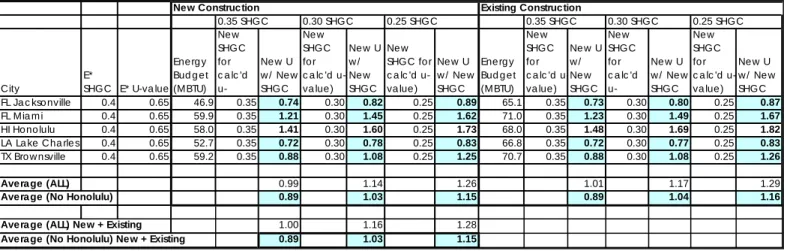
Table A-1 shows results used to determine performance based tradeoffs (Option 2/Table 1) for the South Zone. Figures A-1 through A-6 present this graphically.Table A-1
New Construction Existing Construction
0.35 SHGC 0.30 SHGC 0.25 SHGC 0.35 SHGC 0.30 SHGC 0.25 SHGC City E* SHGC E* U-va lue Ene rg y Bud g e t (MBTU) Ne w SHGC fo r c a lc 'd u-Ne w U w / Ne w SHGC Ne w SHGC fo r c a lc 'd u-va lue ) Ne w U w / Ne w SHGC Ne w SHGC fo r c a lc 'd u-va lue ) Ne w U w / Ne w SHGC Ene rg y Bud g e t (MBTU) Ne w SHGC fo r c a lc 'd u-va lue ) Ne w U w / Ne w SHGC Ne w SHGC fo r c a lc 'd u-Ne w U w / Ne w SHGC Ne w SHGC fo r c a lc 'd u-va lue ) Ne w U w / Ne w SHGC FL Ja c kso nville 0.4 0.65 46.9 0.35 0.74 0.30 0.82 0.25 0.89 65.1 0.35 0.73 0.30 0.80 0.25 0.87 FL Mia m i 0.4 0.65 59.9 0.35 1.21 0.30 1.45 0.25 1.62 71.0 0.35 1.23 0.30 1.49 0.25 1.67 HI Ho no lulu 0.4 0.65 58.0 0.35 1.41 0.30 1.60 0.25 1.73 68.0 0.35 1.48 0.30 1.69 0.25 1.82 LA La ke C ha rle s 0.4 0.65 52.7 0.35 0.72 0.30 0.78 0.25 0.83 66.8 0.35 0.72 0.30 0.77 0.25 0.83 TX Bro w nsville 0.4 0.65 59.2 0.35 0.88 0.30 1.08 0.25 1.25 70.7 0.35 0.88 0.30 1.08 0.25 1.26 Avera ge (ALL) 0.99 1.14 1.26 1.01 1.17 1.29
Avera ge (No Honolulu) 0.89 1.03 1.15 0.89 1.04 1.16
Avera ge (ALL) New + Existing 1.00 1.16 1.28
Avera ge (No Honolulu) New + Existing 0.89 1.03 1.15
In each of the cities in this zone, an energy budget was developed for the current ENERGY STAR criteria (Maximum U and SHGC of .65 and .4 respectively). SHGCs were then dropped to .35, .30, and .25, with resulting U-factors determined for each of the individual climates in order to keep the overall energy budget constant.
Values were determined for New and Existing construction and then averaged. Because the average allowable U-factors with lower SHGCs is higher than the code maximum of 0.8, the tradeoffs are capped at 0.8.
Because the window energy impacts in Honolulu are extremely low, and because the statistical
correlations for Honolulu are poor (especially when lumped in with other climates), Honolulu data was not included in the final U-value calculation for each option.
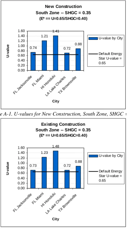
New Construction South Zone -- SHGC = 0.35 (E* == U=0.65/SHGC=0.40) 0.74 1.21 1.41 0.72 0.88 0.00 0.20 0.40 0.60 0.80 1.00 1.20 1.40 1.60 FL J acksonv ille FL Mi ami HI H onolul u LA Lake Char les TX B row nsvil le City U -val ue U-value by City Default Energy Star U-value = 0.65
Figure A-1. U-values for New Construction, South Zone, SHGC = 0.35
Existing Construction South Zone -- SHGC = 0.35 (E* == U=0.65/SHGC=0.40) 0.73 1.23 1.48 0.72 0.88 0.00 0.20 0.40 0.60 0.80 1.00 1.20 1.40 1.60 FL J acksonv ille FL Mi ami HI Honolulu LA L ake C har les TX Br ownsv ille City U -val ue U-value by City Default Energy Star U-value = 0.65
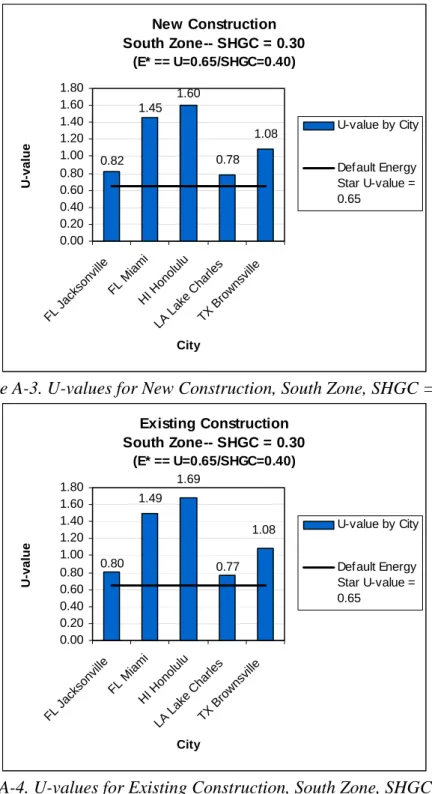
New Construction South Zone-- SHGC = 0.30 (E* == U=0.65/SHGC=0.40) 0.78 1.08 1.45 0.82 1.60 0.00 0.20 0.40 0.60 0.80 1.00 1.20 1.40 1.60 1.80 FL J acksonv ille FL Mi ami HI Honolulu LA L ake C har les TX Br ownsv ille City U -val ue U-value by City Default Energy Star U-value = 0.65
Figure A-3. U-values for New Construction, South Zone, SHGC = 0.30
Existing Construction South Zone-- SHGC = 0.30 (E* == U=0.65/SHGC=0.40) 1.49 1.69 1.08 0.77 0.80 0.00 0.20 0.40 0.60 0.80 1.00 1.20 1.40 1.60 1.80 FL J acksonv ille FL Mi ami HI Honolulu LA L ake C har les TX Br ownsv ille City U -val ue U-value by City Default Energy Star U-value = 0.65
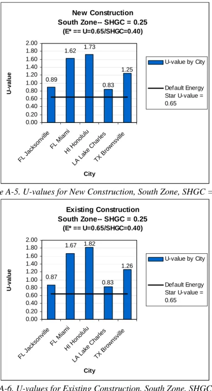
New Construction South Zone-- SHGC = 0.25 (E* == U=0.65/SHGC=0.40) 0.89 1.62 1.73 1.25 0.83 0.00 0.20 0.40 0.60 0.80 1.00 1.20 1.40 1.60 1.80 2.00 FL J acksonv ille FL Mi ami HI Honolulu LA L ake C har les TX B rownsv ille City U -val ue U-value by City Default Energy Star U-value = 0.65
Figure A-5. U-values for New Construction, South Zone, SHGC = 0.25
Existing Construction South Zone-- SHGC = 0.25 (E* == U=0.65/SHGC=0.40) 1.67 0.87 1.26 0.83 1.82 0.00 0.20 0.40 0.60 0.80 1.00 1.20 1.40 1.60 1.80 2.00 FL J acksonv ille FL Mi ami HI Honolulu LA L ake C har les TX B rownsv ille City U -val ue U-value by City Default Energy Star U-value = 0.65
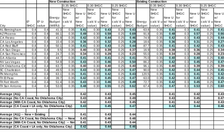
South Central Zone
Table A-2 shows results used to determine performance based tradeoffs (Option 2/Table 1) for the South Central zone. Figures A-7 through A-12 present this graphically.In each of the cities in this zone, an energy budget was developed for the current ENERGY STAR criteria (Maximum U and SHGC of .4 and .4). SHGCs were then dropped to .35, .30, and .25, with resulting U-factors determined for each of the individual climates in order to maintain the overall energy budget.
Values were determined for New and Existing construction and then averaged.
This ENERGY STAR zone includes all of Oklahoma even though some portions of Oklahoma have HDD>3500 (including Oklahoma City.) Including Oklahoma City in the analysis would thus skew results. As a result, it was dropped from the average.
The California climates of San Diego, Los Angeles, and San Francisco are representations of those cities’ coastal climates (cooler and foggier than inland areas). The hotter/sunnier inland areas (where much of the population and housing is) are not well represented by these weather tapes. In order not to bias results for the South Central zone, only the Los Angeles climate was included in the climate averaging.
Table A-2
New Construction Existing Construction
0.35 SHGC 0.30 SHGC 0.25 SHGC 0.35 SHGC 0.30 SHGC 0.25 SHGC City E* SHGC E* U-va lue Ene rg y Bud g e t (MBTU) New SHGC fo r c a lc 'd u-Ne w U w / Ne w SHGC New SHGC fo r c a lc 'd u-va lue ) New U w / New SHGC Ne w SHGC fo r c a lc 'd u-va lue ) Ne w U w / Ne w SHGC Energ y Bud g e t New SHGC fo r c a lc 'd u-va lue) New U w / Ne w SHGC Ne w SHGC for c a lc 'd u-va lue) New U w / New SHGC Ne w SHGC for c a lc 'd u-va lue ) Ne w U w / Ne w SHGC AL Birm ing ha m 0.4 0.4 41.3 0.35 0.41 0.30 0.43 0.25 0.43 63.8 0.35 0.41 0.3 0.41 0.25 0.41 AZ Phoe nix 0.4 0.4 66.1 0.35 0.49 0.30 0.59 0.25 0.69 91.8 0.35 0.48 0.3 0.57 0.25 0.66 CA Fre sno 0.4 0.4 41.9 0.35 0.42 0.30 0.44 0.25 0.46 74.9 0.35 0.42 0.3 0.43 0.25 0.44 CA Los Ang e le s 0.4 0.4 10.4 0.35 0.36 0.30 0.32 0.25 0.28 18.6 0.35 0.36 0.3 0.31 0.25 0.27 CA Red Bluff 0.4 0.4 50.1 0.35 0.41 0.30 0.43 0.25 0.44 87.7 0.35 0.41 0.3 0.42 0.25 0.43 CA Sa n Die g o 0.4 0.4 9.5 0.35 0.40 0.30 0.39 0.25 0.37 16.9 0.35 0.38 0.3 0.36 0.25 0.34 CA Sa n Fra nc isc o 0.4 0.4 24.7 0.35 0.34 0.30 0.29 0.25 0.23 55.0 0.35 0.34 0.3 0.28 0.25 0.23 GA Atla nta 0.4 0.4 44.7 0.35 0.41 0.30 0.41 0.25 0.41 75.0 0.35 0.40 0.3 0.40 0.25 0.40 NV La s Veg a s 0.4 0.4 54.9 0.35 0.43 0.30 0.46 0.25 0.50 86.2 0.35 0.42 0.3 0.45 0.25 0.47 OK Okla ho m a City 0.4 0.4 63.7 0.35 0.40 0.30 0.40 0.25 0.40 96.1 0.35 0.40 0.3 0.39 0.25 0.39
SC Cha rle sto n 0.4 0.4 49.5 0.35 0.43 0.30 0.45 0.25 0.47 90.0 0.35 0.42 0.3 0.44 0.25 0.45
TN Me m p his 0.4 0.4 63.1 0.35 0.41 0.30 0.42 0.25 0.43 120.5 0.35 0.41 0.3 0.41 0.25 0.42
TX El Pa so 0.4 0.4 39.7 0.35 0.42 0.30 0.45 0.25 0.47 63.0 0.35 0.42 0.3 0.43 0.25 0.45
TX Fort Worth 0.4 0.4 51.4 0.35 0.43 0.30 0.46 0.25 0.49 72.7 0.35 0.42 0.3 0.45 0.25 0.47
TX Sa n Antonio 0.4 0.4 53.0 0.35 0.48 0.30 0.55 0.25 0.62 67.4 0.35 0.47 0.3 0.53 0.25 0.60
Avera ge (ALL) 0.42 0.43 0.45 0.41 0.42 0.43
Avera ge (No CA Coast, No Oklahoma City) 0.43 0.46 0.49 0.43 0.45 0.47
Avera ge (With CA Coa st, No Okla homa City) 0.42 0.43 0.45 0.41 0.42 0.43
Avera ge (CA Coa st = LA only, No Okla homa City) 0.43 0.45 0.47 0.42 0.44 0.46
Avera ge (ALL) -- New + Existing 0.41 0.43 0.44
Avera ge (No CA Coast, No Oklahoma City) -- New 0.43 0.46 0.48
Avera ge (With CA Coa st, No Okla homa City) -- New 0.41 0.43 0.44
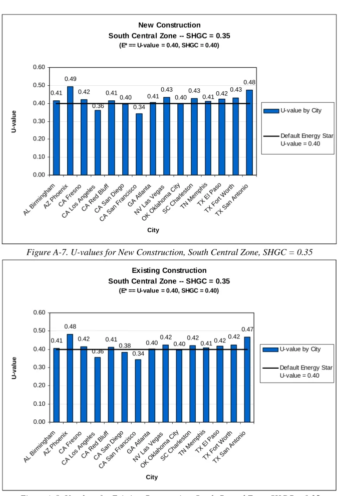
New Construction
South Central Zone -- SHGC = 0.35
(E* == U-value = 0.40, SHGC = 0.40) 0.41 0.49 0.42 0.41 0.43 0.43 0.48 0.43 0.42 0.41 0.40 0.41 0.40 0.34 0.36 0.00 0.10 0.20 0.30 0.40 0.50 0.60 AL B irmi ngham AZ PhoenixCA F res no CA Los Ange les CA Red Bl uff CA San Diego CA S an Fr anc isco GA Atlanta NV Las Vega s OK O klah oma Cit y SC Char leston TN Memp his TX El P aso TX F ort Wor th TX San Antonio City U -val ue U-value by City
Default Energy Star U-value = 0.40
Figure A-7. U-values for New Construction, South Central Zone, SHGC = 0.35
Existing Construction South Central Zone -- SHGC = 0.35
(E* == U-value = 0.40, SHGC = 0.40) 0.41 0.48 0.42 0.41 0.42 0.42 0.47 0.42 0.42 0.41 0.40 0.40 0.38 0.34 0.36 0.00 0.10 0.20 0.30 0.40 0.50 0.60 AL Birmingham AZ PhoenixCA F resno CA Los Ange les CA Red Bluff CA S an Di ego CA S an F ranc isco GA A tlanta NV Las Vegas OK Ok lahoma Cit y SC Cha rleston TN Memphi s TX El Paso TX F ort W orth TX San Antonio City U -val ue U-value by City
Default Energy Star U-value = 0.40
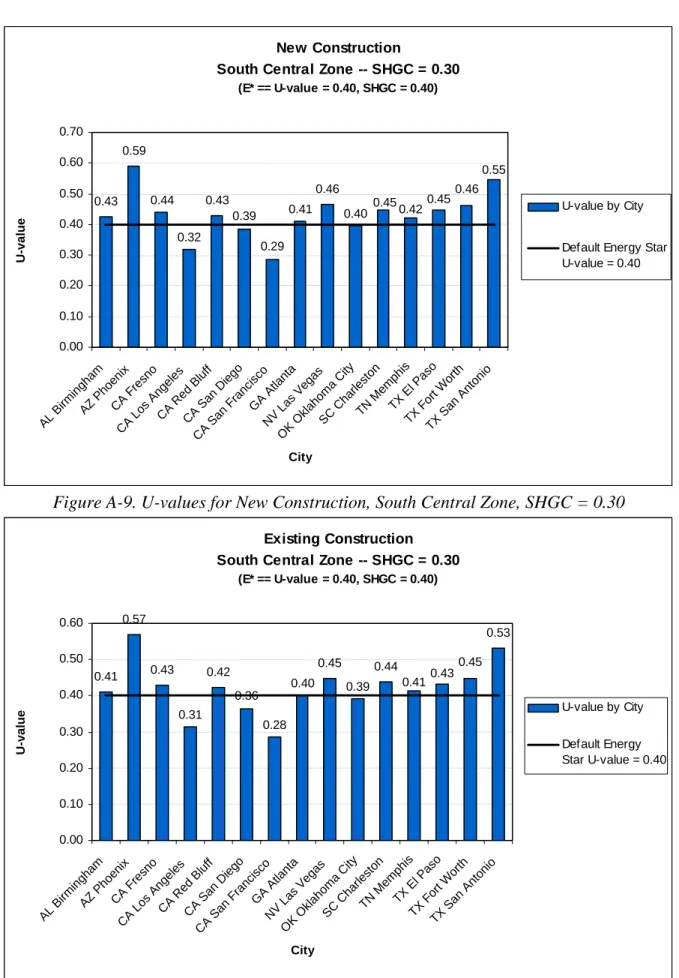
New Construction
South Central Zone -- SHGC = 0.30
(E* == U-value = 0.40, SHGC = 0.40) 0.43 0.59 0.43 0.46 0.55 0.45 0.44 0.450.46 0.42 0.40 0.41 0.39 0.29 0.32 0.00 0.10 0.20 0.30 0.40 0.50 0.60 0.70 AL Birmingham AZ Phoeni x CA Fr esno CA Los Angel es CA Re d B luff CA S an Di ego CA San F ranci sco GA Atl anta NV Las Vegas OK Ok lahoma C ity SC C har les ton TN Memp his TX E l Paso TX F ort W orth TX San Antoni o City U-v a lue U-value by City
Default Energy Star U-value = 0.40
Figure A-9. U-values for New Construction, South Central Zone, SHGC = 0.30
Existing Construction South Central Zone -- SHGC = 0.30
(E* == U-value = 0.40, SHGC = 0.40) 0.41 0.57 0.43 0.42 0.45 0.44 0.53 0.31 0.28 0.36 0.40 0.39 0.410.43 0.45 0.00 0.10 0.20 0.30 0.40 0.50 0.60 AL Birmingham AZ Phoeni x CA Fr esno CA Los Ange les CA Red BluffCA S an Di ego CA San F ranci sco GA Atl anta NV Las Vegas OK O klahoma Cit y SC Char leston TN Memphi s TX E l Paso TX F ort W orth TX San Antoni o City U-v a lue U-value by City Default Energy Star U-value = 0.40
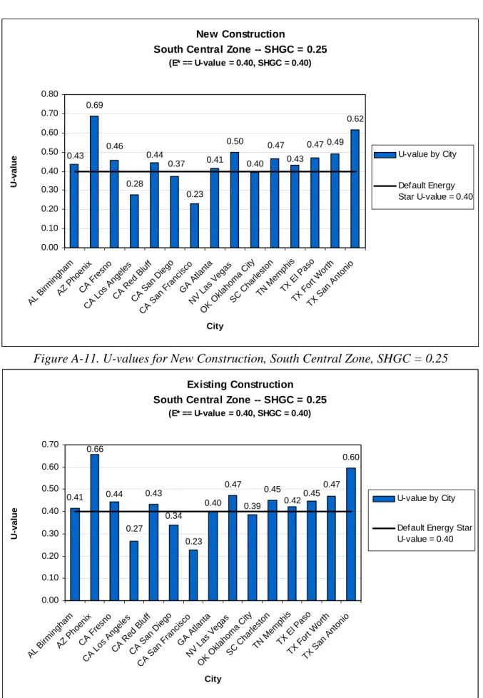
New Construction
South Central Zone -- SHGC = 0.25
(E* == U-value = 0.40, SHGC = 0.40) 0.69 0.50 0.62 0.43 0.46 0.47 0.44 0.28 0.23 0.37 0.41 0.40 0.43 0.47 0.49 0.00 0.10 0.20 0.30 0.40 0.50 0.60 0.70 0.80 AL Bi rmi ngham AZ Phoeni x CA F resno CA Los Angel es CA Re d B luff CA S an Di ego CA San Fr anc isco GA Atlanta NV Las Veg as OK Ok lahoma C ity SC C har les ton TN Memp his TX El Paso TX F ort W orth TX S an A ntoni o City U-v a lue U-value by City Default Energy Star U-value = 0.40
Figure A-11. U-values for New Construction, South Central Zone, SHGC = 0.25
Existing Construction South Central Zone -- SHGC = 0.25
(E* == U-value = 0.40, SHGC = 0.40) 0.41 0.43 0.47 0.45 0.60 0.66 0.44 0.47 0.45 0.42 0.39 0.40 0.34 0.23 0.27 0.00 0.10 0.20 0.30 0.40 0.50 0.60 0.70 AL Birmingham AZ PhoenixCA F res no CA Los Angeles CA Red Bluff CA S an Di ego CA San F ranci sco GA A tlanta NV Las Vega s OK Ok lahoma Cit y SC Cha rleston TN Memphi s TX E l Pas o TX For t Wo rth TX San Antonio City U -val ue U-value by City
Default Energy Star U-value = 0.40
North Central Zone
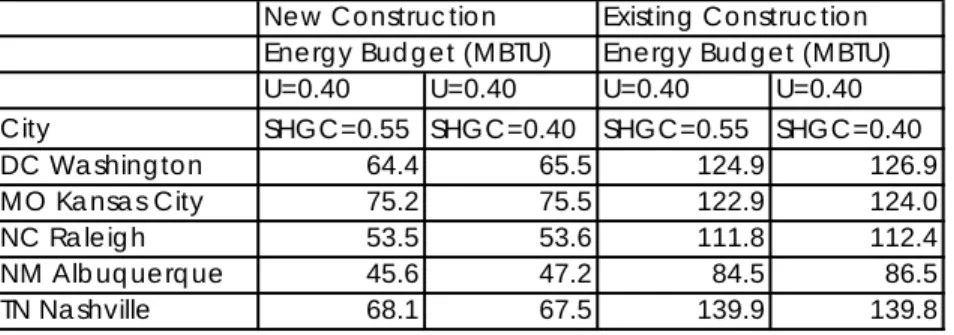
Table A-3 shows total energy use data for a selection of the North Central Zone cities.This table, along with the corresponding figures (A-13 and A-14) shows that for a fixed U-factor,
different SHGCs produce no discernable impact on total energy use. This is due to the fact that climates in this zone have approximately equal heating and cooling loads from windows. Where solar gains help with reducing winter heating loads, they also detract approximately equally from cooling loads.
Table A-3
Ne w Co nstruc tio n Existing Co nstruc tio n Ene rg y Bud g e t (MBTU) Ene rg y Bud g e t (MBTU)
U=0.40 U=0.40 U=0.40 U=0.40
City SHGC=0.55 SHGC=0.40 SHGC=0.55 SHGC=0.40 DC Wa shing to n 64.4 65.5 124.9 126.9 MO Ka nsa s City 75.2 75.5 122.9 124.0 NC Ra le ig h 53.5 53.6 111.8 112.4 NM Alb uq ue rq ue 45.6 47.2 84.5 86.5 TN Na shville 68.1 67.5 139.9 139.8
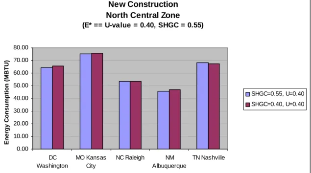
New Construction North Central Zone (E* == U-value = 0.40, SHGC = 0.55) 0.00 10.00 20.00 30.00 40.00 50.00 60.00 70.00 80.00 DC Washington MO Kansas City NC Raleigh NM Albuquerque TN Nashville
Energy Consumption (MBTU)
SHGC=0.55, U=0.40 SHGC=0.40, U=0.40
Figure A-13. Energy Budgets for New Construction, North Central Zone, for U-value = 0.40 and SHGC = 0.40 and 0.55
Existing Construction North Central Zone (E* == U-value = 0.40, SHGC = 0.55) 0.00 20.00 40.00 60.00 80.00 100.00 120.00 140.00 160.00 DC Washington MO Kansas City NC Raleigh NM Albuquerque TN Nashville
Energy Consumption (MBTU)
SHGC=0.55, U=0.40 SHGC=0.40, U=0.40
Figure A-14. Energy Budgets for Existing Construction, North Central Zone, for U-value = 0.40 and SHGC = 0.40 and 0.55
North Zone
Table A-4 shows total energy use data for a selection of North Zone cities, including 4 Canadian cities.This table, along with corresponding Figures A-15 and A-16, shows, for a fixed U=.35, the impacts of two different SHGCs (.55 and .40) on total energy use. Total annual energy use is slightly lower with the higher SHGC product due to the fact that increased solar heat gain decreases heating loads more than cooling loads are increased.
No tradeoffs are proposed for this northern zone because a base SHGC has not been defined by the ENERGY STAR program (see Base SHGC in the North subsection in the text of the white paper).
Table A-4
Ne w Co nstruc tio n Existing Co nstruc tio n Ene rg y Bud g e t (MBTU) Ene rg y Bud g e t (MBTU)
U=0.35 U=0.35 U=0.35 U=0.35
City SHGC=0.55 SHGC=0.40 SHGC=0.55 SHGC=0.40 AK Anc ho ra g e 110.4 116.0 241.5 248.7 CO De nve r 56.4 59.5 127.5 131.7 ID Bo ise 65.1 67.5 127.8 131.2 IL Chic a g o 79.8 81.8 149.9 153.2 MA Bo sto n 72.7 75.8 129.8 134.1 ME Po rtla nd 76.7 81.5 154.2 160.5 MN Minne a p o lis 98.2 101.3 182.2 186.8 MT Gre a t Fa lls 88.6 92.6 177.0 182.5 ND Bism a rk 98.8 102.7 199.7 205.2 NE Om a ha 81.6 83.0 146.2 148.7 NV Re no 49.4 52.3 97.2 101.0 NY Buffa lo 83.6 86.1 169.2 173.1 NY Ne w Yo rk 66.7 68.6 127.1 129.8 OH Da yto n 72.5 74.7 133.9 137.2 OR Me d fo rd 50.7 51.9 122.0 123.7 OR Po rtla nd 45.9 48.1 114.7 117.7 PA Phila d e lp hia 65.6 67.3 126.3 128.8 PA Pittsb urg h 70.9 72.7 140.4 143.3 UT Sa lt La ke City 61.7 63.3 128.2 130.7 VT Burling to n 88.4 92.2 170.9 176.3 WA Se a ttle 48.3 51.6 100.3 104.8 WI Ma d iso n 85.8 89.0 163.6 168.2 WY Che ye nne 76.2 81.5 169.8 176.6 ON To ro nto 83.5 86.6 164.9 169.6 PQ Mo ntre a l 97.3 100.9 191.4 196.6 AB Ed m o nto n 117.6 123.8 255.3 263.5 NS Ha lifa x 85.1 90.5 178.9 185.7
New Construction North Zone
(E* == U-value = 0.35, SHGC = N/A)
0 20 40 60 80 100 120 140 AK Anc hor age CO Denv er ID Bois e IL ChicagoMA Bos ton ME Por tlan d MN Mi nneapol is MT Gre at Fall s ND Bi smar k NE O maha NV Reno NY Buffalo NY New York OH Dayton OR Medfor d OR Por tlan d PA Phi lad elphia PA Pitts burgh UT Sal t Lake Ci ty VT Bur lingt on WA Seattle WI Madis on WY Che yenne
Energy Consumption (MBTU)
SHGC=0.55, U=0.35 SHGC=0.40, U=0.35 v
Figure A-15. Energy Budgets for New Construction, North Zone, for U-value = 0.35 and SHGC = 0.40 and 0.55
Existing Construction North Zone
(E* == U-value = 0.35, SHGC = N/A)
0 50 100 150 200 250 300 AK A ncho rage CO Den ver ID Bo ise IL C hicag o MA Bost on ME Portl and MN Min neapo lis MT Grea t Falls ND Bisma rk NE Oma ha NV Reno NY Buffa lo NY New Yor k OH Day ton OR Med ford OR Po rtlan d PA Phila delph ia PA Pitt sburg h UT Salt La ke C ity VT Burlin gton WA Seat tle WI Ma diso n WY Chey enn e
Energy Consumption (MBTU)
SHGC=0.55, U=0.35 SHGC=0.40, U=0.35
Figure A-16. Energy Budgets for Existing Construction, North Zone, for U-value = 0.35 and SHGC = 0.40 and 0.55