DISTRIBUTED PARALLEL PROCESSING AND DYNAMIC LOAD BALANCING TECHNIQUES FOR MULTIDISCIPLINARY HIGH SPEED AIRCRAFT DESIGN
by
Denitza T. Krasteva
Thesis submitted to the Faculty of the Virginia Polytechnic Institute and State University in partial fulfillment of the requirements for the degree of
MASTER OF SCIENCE
in
Computer Science and Applications
APPROVED:
Layne T. Watson
Dennis G. Kafura Rakesh K. Kapania
September, 1998 Blacksburg, Virginia
DISTRIBUTED PARALLEL PROCESSING AND DYNAMIC LOAD BALANCING TECHNIQUES FOR MULTIDISCIPLINARY HIGH SPEED AIRCRAFT DESIGN
by
Denitza T. Krasteva
Committee Chairman: Layne T. Watson Computer Science
(ABSTRACT)
Multidisciplinary design optimization (MDO) for large-scale engineering problems poses many challenges (e.g., the design of an efficient concurrent paradigm for global optimization based on disciplinary analyses, expensive computations over vast data sets, etc.) This work focuses on the application of distributed schemes for massively parallel architectures to MDO problems, as a tool for reducing computation time and solving larger problems. The specific problem considered here is configuration optimization of a high speed civil transport (HSCT), and the efficient parallelization of the embedded paradigm for reasonable design space identification. Two distributed dynamic load balancing techniques (random polling and global round robin with message combining) and two necessary termination detection schemes (global task count and token passing) were implemented and evaluated in terms of effectiveness and scalability to large problem sizes and a thousand processors. The effect of certain parameters on execution time was also inspected. Empirical results demonstrated stable performance and effectiveness for all schemes, and the parametric study showed that the selected algorithmic parameters have a negligible effect on performance.
ACKNOWLEDGEMENTS.
During the course of this work I have had the advantage of receiving academic support from my advisor, Dr. Layne Watson and the professors and students from the MDO group— Dr. Bernard Grossman, Dr. William Mason, Dr. Raphael Haftka, and Chuck Baker. Many thanks go to Dr. Watson who provided the initial stimulus for this work. His guidance has facilitated a rich educational experience for me through numerous discussions, valuable advice and direction, encouragement, and fair criticism. I am very happy that I had the chance to have Dr. Watson as my academic advisor. I would also like to thank Dr. Grossman, Dr. Mason and Chuck Baker for their support and discussions during the weekly MDO meetings, and Dr. Haftka for his invaluable advice and critique of my work. Finally, Dr. Kafura is the professor to whom I am grateful for sparking my interest in concurrency and distributed systems issues during his Advanced Concepts in Operating Systems class.
My deepest gratitude goes to my parents, Chavdar Krastev and Pollina Krasteva, and family who have patiently provided me with unfailing support, encouragement and care even though they were not physically here. I am very thankful to my grandparents, who showed constant interest in every step of my progress. Chris Gale is responsible for making my stay in Blacksburg wonderful, and for making me feel good at times when I had little reason to do so. Finally, I would like to pay tribute to all my friends and collegues who contributed to creating a great educational and personal atmosphere for me.
Financially, this work was supported in part by Air Force Office of Scientific Research grant F49620-92-J-0236, National Science Foundation grant DMS-9400217, and National Aeronautics and Space Administration grant NAG-2-1180. I would also like to gratefully acknowledge the use of the Intel Paragon XP/S 5, XP/S 35, and XP/S 150 computers, located in the Oak Ridge National Laboratory Center for Computational Sciences (CCS), funded by the Department of Energy’s Mathematical, Information, and Computational Sciences (MICS) Division of the Office of Computational and Technology Research. A lot of the results described in this thesis were obtained from runs on these computers.
TABLE OF CONTENTS 1. Introduction . . . 1 2. HSCT Configuration Optimization . . . 5 2.1 Design Variables . . . 7 2.2 Constraints . . . 7 2.3 Multi-fidelity Analysis . . . 11
3. Reasonable Design Space Paradigm . . . 12
3.1 Design of Experiments Theory . . . 12
4. Parallelization Strategy . . . 14 4.1 Parallel Implementation . . . 15 4.1.1 MPI . . . 15 4.1.2 Threads . . . 16 5. Distributed Algorithms . . . 18 5.1 Assumptions . . . 18
5.2 Dynamic Load Balancing . . . 19
5.2.1 Random Polling . . . 19
5.2.1 Global Round Robin with Message Combining . . . 20
5.3 Termination Detection . . . 21
5.3.1 Global Task Count . . . 22
5.3.2 Token Passing . . . 23
6. Parallel Performance . . . 25
7. Parametric Study . . . 30
8. Conclusions and Future Work . . . 35
References . . . 36
Appendix B: Code for Worker Thread . . . 50
Appendix C: Code for GRR-MC Thread . . . 55
Appendix D: Design Variable Definition File Used for Test Runs . . . 68
Vita . . . 69
LIST OF FIGURES Figure 1. Typical HSCT configuration . . . 6
Figure 2. Wing planform design variables . . . 8
Figure 3. Wing airfoil thickness design variables . . . 8
Figure 4. GRR-MC spanning tree forN = 8, where x is the value of T . . . 21
Figure 5. Snapshot from nupshot utility of static load distribution,N = 7 . . . 26
Figure 6. Snapshot fromnupshotutility of GRR-MC with GTC termination,N = 7 26 Figure 7. Snapshot from nupshot utility of RP with GTC termination,N = 7 . . . 26
Figure 8. Speedup with base N = 32 for RP and GRR-MC with global task count termination, on N = 2{5...10} processors . . . . 28
Figure 9. Speedup with base N = 32 for RP and GRR-MC with token passing termi-nation, on N = 2{5...10} processors . . . 28
Figure 10. Effect of transfer threshold for N = 32 on 30,915 designs . . . 32
Figure 11. Effect of transfer threshold for N = 64 on 30,915 designs . . . 32
Figure 12. Effect of splitting ratioα forN = 32 on 30,915 designs . . . 33
Figure 13. Effect of splitting ratioα forN = 64 on 30,915 designs . . . 33
Figure 14. Effect of splitting ratio on RP GTC for N = 64 on 2,026,23 designs . . 34
Figure 15. Effect of transfer threshold on RP TP forN = 64 on 2,026,23 designs 34 LIST OF TABLES Table 1. Design variables and typical values . . . 9
Table 2. Optimization Constraints . . . 10
Table 3. Intel Paragon parallel times (hh:mm:ss) for low fidelity analysis of 2,026,231 HSCT designs . . . .25
1. INTRODUCTION.
The requirement for timely deliverance, in the context of inherent computational com-plexity and huge problem size spanning several disciplines, is typical of modern large-scale engineering problems (e.g., aircraft design). This has provided the driving force for research in the area of multidisciplinary design optimization (MDO) to develop practical, scalable methodologies for design optimization and analysis from the perspective of more than one discipline. The computational intensity of realistic multidisciplinary design optimization problems presents a major obstacle and bottleneck. For this reason, high performance com-puting and its efficient use constitute a very important MDO tool. There is an ongoing effort amongst engineering and scientific computing researchers to build sophisticated parallel and distributed algorithms for the solutions of specific types of problems, such as computational fluid dynamics (CFD), partial differential equations (PDEs), finite element analysis, etc. (see, for example, the July 1998 issue of Advances in Engineering Software). Despite their good performance and promising potential, such codes are not widely integrated in MDO environments, since it is a nontrivial task to efficiently blend heterogeneous, disciplinary engineering codes together. Obstacles that arise are complex interactions between disciplines, incompatible interfaces, nonstandard programming practices, lack of detailed documenta-tion, and sometimes failure to scale up to the sizes of realistic MDO problems. As a result, more customization is needed than is feasible. Burgee et al. [7] discuss similar difficulties in their effort to parallelize sequential MDO codes composed of legacy disciplinary analysis codes.
Several efforts are described in the literature that propose parallel and distributed solutions to the complexity and computational burden of large scale MDO problems. One strain of research develops methodologies for MDO problem modeling and formulation with the goal of creating significant opportunities for distributed and parallel computation. Kroo et al. [24] propose two such methodologies. One is the decomposition of analyses into simpler modules with limited interdependencies, so that each module can be run concurrently. Collaborative optimization [5], on the other hand, aims at modeling the entire design process as a collaboration between parallel tasks/disciplines, under the auspices of
a centralized coordinating process. Dennis and Lewis introduce the “individual discipline feasible” [8] problem formulation approach for MDO that has the advantage of using third party disciplinary analysis codes. There is work at Georgia Tech on agent based technologies for the IMAGE infrastructure of their decision support integrated product and process development (IPPD) architecture DREAMS [15]. The applicability and scalability of the above methods for large-scale systems has yet to be established.
A second strain of research is oriented towards the design and implementation of generic MDO computing frameworks that support concurrent execution across distributed, heterogeneous platforms (see Access Manager [27], COMETBOARDS [18], and Fido [34]). For example, Wujek et al. [35] propose a framework, later extended by Yoder and Brockman [36], that facilitates distributed collaborative design [24] and manages the entire problem-solving life-cycle through a graphical user interface. These systems aim to automate the design optimization process by controlling computing processes, and tracking and monitoring intermediate results. Their problem definition capabilities need to be very flexible and robust in order to accommodate complex MDO problems. Additionally, tracking and monitoring tools like FIDO’s Spy [34] are very important to keep the designer informed about the state of the optimization, and to allow the designer to interact with the automated process. Currently, more empirical evidence is needed to show if automated, “push-button” (see Dennis and Lewis [8]) systems are well suited to large, complex MDO problems.
Finally, there has been research on using sophisticated parallel algorithms for different MDO subproblems such as optimization, analysis, etc. For example, Burgee et al. [7] and Balabanov et al. [1] implemented coarse-grained parallel versions of existing analysis and optimization codes for a High Speed Civil Transport. The results were reasonable, but speedup tapered off for less than 100 nodes, due to I/O overhead, and other factors discussed in [7], [1]. Their conclusion was that fine-grained parallelism and reduced I/O versions of the codes would improve scalability. There are some reports of efficiency achieved on massively parallel architectures, i.e., scalability to thousands of nodes. For example, Dennis and Torczon [9] developed the parallel direct search methods for derivative free optimization that are blatantly parallel. Direct search methods are suitable for problems with a relatively small number
of design variables (<50). Ghattas and Orozco have developed a parallel reduced Hessian sequential quadratic programming (SQP) method for shape optimization [12] that scales very well up to thousands (16000) of processors for relatively small numbers of design variables (<50), but performance quickly degrades as the number of design variables increases. Eldred et al. [11] have developed an object oriented software framework for generic optimization that experienced optimal performance at 512 processors for a certain test problem, but started degrading after that. More research seems to focus on moderate parallelism, i.e., less than 100 processors. For example, Jameson et al. [20] assess parallel implementations of an algorithm applying control theory to CFD aerodynamic optimization. Reported efficiencies range between 66 and 95 percent, but the need for more effective load balancing is recognized and the focus of current study. For more research on parallel and distributed MDO tools, including parallel genetic algorithms using MPI [31], and Java based solutions, see [19], [3], [10], [2].
This paper focuses on the effective use of massive parallelism and scalable distributed control applied to the reasonable design space identification paradigm embedded within the problem of the multidisciplinary configuration optimization of a High Speed Civil Transport (HSCT). The approach here uses a variable complexity paradigm [7] where computation-ally cheap low fidelity techniques are used together with computationcomputation-ally expensive high fidelity techniques throughout the optimization process. Geometric constraints and low fidelity analysis are applied to define promising regions in the design space and to identify intervening/important variables/terms for surrogate models. Higher fidelity analyses are used to generate smooth response surfaces for those regions, which are then analyzed by the optimizers in search of local optima. Typical configuration designs are comprised of 5 to 50 design variables.
The paradigm of reasonable design space identification consists of performing millions of low fidelity analyses at extreme points of a box around a nominal configuration. A single design evaluation takes a fraction of a second on a slow processor, but as the number of design variables grows, millions of evaluations require a significant amount of time. Such an evaluation is too fine grained to lend itself to task parallelism, and so is taken as the
atomic grain of computation. In terms of data parallelism, the problem is irregular because each configuration that fails preliminary analysis (violates feasibility constraints) has to be moved towards the center of the box until it is coerced to a reasonable design. This results in a variable number of analyses and time per configuration. Initially, a parallel implementation was developed where all configurations to be evaluated were spread evenly across available processors. A severe load imbalance, where total idle time amounted to one half of total processing time, was observed. Thus dynamic load balancing strategies, so that the load can be effectively redistributed amongst processors at run time, are essential. Two receiver initiated distributed load balancing algorithms—random polling (RP) and global round robin with message combining (GRR-MC)—were implemented.
Load balancing causes remapping of jobs to processors so that processors that have finished their work at some point in time can resume with a new load. Thus a processor having no load at a certain point in time does not signify that there is no more work to be done on a global level. A termination detection algorithm is needed to assert global termination of the system. Two complementary termination detection schemes—global task count (GTC) and token passing (TP)—have been implemented. The parallel codes make use of the Message Passing Protocol (MPI) [31] for interprocessor and collective communication, and POSIX threads (pthreads) for concurrency at the processor level. To provide context, the HSCT aircraft design problem is described in detail in Chapter 2. Chapter 3 describes the reasonable design space paradigm, Chapters 4 and 5 the algorithms and their implementation. Chapters 6 and 7 analyze the results and parametric studies, and Chapter 8 offers conclusions and possible future work.
2. HSCT CONFIGURATION OPTIMIZATION.
The parallelization techniques described in the following chapters are applied in the context of designing an optimal supersonic aircraft with a capacity for 251 passengers, minimum range of 5,500 nautical miles, cruise speed of Mach 2.4, and ceiling height of 70,000 ft. The problem is formulated as a constrained optimization
min
xmin≤x≤xmax
f(x), subject to gi(x)≤0 for all i∈ {1, . . . , m},
where f :Rn →R is the objective function, x∈Rn is a vector of ndesign variables, and
g:Rn →Ris a vector of m constraints. The values of the design variables in vectorx are lower and upper bounded by xmin and xmax respectively.
Takeoff gross weight (TOGW), expressed as the aggregate of payload, fuel, structural and nonstructural weights, serves as the selected objective function. TOGW is dependent on many of the engineering disciplines involved, (e.g., structural design determines empty aircraft weight, aerodynamic design affects required fuel weight, etc.), and thus provides a measure of merit for the HSCT as a whole. Guinta [13] suggests that minimized takeoff gross weight is also in some sense related to minimized acquisition and recurring costs for the aircraft. Figure 1 [23] illustrates a typical aircraft configuration.
The suite of optimization and analysis tools employed for this problem comprises codes developed by engineers in-house (e.g., vortex lattice subsonic aerodynamics, panel code for supersonic aerodynamics) and by third parties (e.g., optimizer, weights and structures, Harris [16] wave drag code for supersonic aerodynamics). The analysis tools are of varying complexity and computational expense, and some have coarse-grained parallel implementa-tions. Interactions and coordination amongst programs in the suite are mostly carried out via file I/O.
2.1. DESIGN VARIABLES.
Successful aircraft design optimization requires a suitable mathematical characterization of configuration parameters. Typically a configuration has n≤50 design variables. In this particular case, 29 variables are used to define the HSCT in terms of geometric—wing-body-nacelle—layout (twenty six variables) and mission profile (three variables). See Table 1 [13] for descriptions and typical values of all design variables. The wing is parametrized with eight variables for planform (see Figure 2 [13]) and five variables for leading edge and airfoil shape properties (see Figure 3 [13]). Two variables express the engine nacelle locations along the wing semi-span. The fuselage shape is defined with eight variables specifying the axial location and radius for each of four restraint points along its fixed 300 ft length. The horizontal and vertical tails are trapezoidal planforms whose areas each comprise a design variable. The thrust of the engine is also a variable. Internal volume of the aircraft is fixed at 23,270 ft3.
The idealized mission profile is divided into three segments—takeoff, supersonic leg at Mach 2.4, and landing. There are three variables related to the mission—flight fuel weight, climb rate, and initial supersonic cruise/climb altitude.
2.2. CONSTRAINTS.
The HSCT optimization process is subject to 69 explicit nonlinear constraints of vary-ing complexity and computational expense. The least expensive to evaluate are geometric constraints that are used to eliminate physically senseless designs involving negative lengths, zero thickness, etc. Aerodynamic and performance constraints vary from moderately expen-sive (e.g., stability issues) to computationally intenexpen-sive (range ≥5,500). Table 2 [13] lists all constraints with short descriptions.
8 x22 23 x x 5 x x x x7 6 1 (x 2, x ) 4, x ) y fuselage centerline 3 (x
Figure 2. Wing planform design variables.
x
t/c ratio at 3 spanwise locations
10 LE radius x9 max. thickness location x
11--13 x
z
Table 1. Design variables and typical values.
Index Typical Value Description
1 181.48 Wing root chord
2 155.90 LE break point, x (ft)
3 49.20 LE break point, y (ft)
4 181.60 TE break point,x (ft)
5 64.20 TE break point,y (ft)
6 169.50 LE wing tip, x (ft)
7 7.00 Wing tip chord (ft)
8 74.90 Wing semi-span (ft)
9 0.40 Chordwise location of max. thickness
10 3.69 LE radius parameter
11 2.58 Airfoilt/c ratio at root, (%)
12 2.16 Airfoilt/c ratio at LE break, (%)
13 1.80 Airfoilt/c ratio at LE tip, (%)
14 2.20 Fuselage restraint 1, x (ft) 15 1.06 Fuselage restraint 1, y (ft) 16 12.20 Fuselage restraint 2, x (ft) 17 3.50 Fuselage restraint 2, y (ft) 18 132.46 Fuselage restraint 3, x (ft) 19 5.34 Fuselage restraint 3, y (ft) 20 248.67 Fuselage restraint 4, x (ft) 21 4.67 Fuselage restraint 4, y (ft) 22 26.23 Nacelle 1 location (ft) 23 32.39 Nacelle 2 location (ft)
24 697.90 Vertical tail area (ft2)
25 713.00 Horizontal tail area (ft2)
26 39000.00 Thrust per engine (lb)
27 322617.00 Flight fuel (lb)
28 64794.00 Starting cruise/climb altitude (ft)
Table 2. Optimization constraints.
Index Constraint
Geometric Constraints
1 Fuel volume≤50% wing volume 2 Airfoil section spacing at Ctip ≥3.0 ft
3–20 Wing chord ≥7.0 ft
21 LE break within wing semi-span 22 TE break within wing semi-span 23 Root chordt/c ratio ≥1.5% 24 LE break chord t/c ratio≥1.5% 25 Tip chord t/c ratio≥1.5% 26–30 Fuselage restraints
31 Nacelle 1 outboard of fuselage 32 Nacelle 1 inboard of nacelle 2 33 Nacelle 2 inboard of semi-span
Aerodynamic/Performance Constraints
34 Range≥5500 nautical miles 35 CL at landing speed≤1
36–53 Section CL at landing ≤2
54 Landing angle of attack≤12◦ 55–58 Engine scrape at landing
59 Wing tip scrape at landing 60 LE break scrape at landing 61 Rudder deflection ≤22.5◦ 62 Bank angle at landing ≤5◦
63 Tail deflection at approach ≤22.5◦ 64 Takeoff rotation to occur≤Vmin
65 Engine-out limit with vertical tail 66 Balanced field length ≤11000 ft
2.3. MULTI-FIDELITY ANALYSIS.
Minimizing TOGW requires a large number of disciplinary analyses (e.g., structural, aerodynamic), so that the optimal configuration(s) can be found. The computational cost of sophisticated analysis techniques becomes prohibitive as the number of design variables grows (≥ 5), and simpler methods are not accurate enough. A multi-fidelity approach employs methods of varying complexity and computational cost, so that optimization becomes feasible.
Initially, the reasonable design space paradigm employs geometric and low-fidelity analyses to constrain the design space, so that many grossly unreasonable configurations are excluded. The resulting space is called the reasonable design space. High fidelity analyses are then used to construct polynomial approximations, referred to as response surfaces, for the reasonable region. The optimizer works with response surfaces instead of the actual high fidelity analyses, because the former smooth out numerical noise and once generated are much faster and simpler to work with. Additionally, more than one response surface can be generated concurrently.
Unfortunately, the complexity and accuracy of polynomial approximations are adversely affected as the number of design variables increases (≥ 20). For this reason, low fidelity analyses are used to reduce the dimensionality and cost of polynomial models by identifying intervening variables and important terms to be used in reduced term models.
3. REASONABLE DESIGN SPACE PARADIGM.
Defining the reasonable design space consists of evaluating configurations at extreme points (vertices) in a box that contains the region of interest. At these extreme points, designs are found that often prove to be nonsensical on the basis of geometrical constraints or from estimates of the objective function and constraints based on low-fidelity analyses. These low fidelity analyses cannot accurately evaluate constraints, but they allow identification of points that are obviously meaningless. Unreasonable designs are then moved towards the center of the box, using a linear bisection algorithm, until they are no longer in gross violation of the constraints. The edge of the reasonable design space is determined in this manner.
3.1. DESIGN OF EXPERIMENTS THEORY.
A point selection algorithm is needed to generate the configurations from the box—a
p-cube, centered at the origin, where pis the number of design variables—that will be used to define the reasonable design space. A full factorial design is a possible choice, but it will result in an unwieldy number of configurations. For example, a 25 variable problem with two levels for each design variable results in 225≈33 million points. With an average of three
evaluations needed to bring a point to the reasonable design space, this would require about 100 million low-fidelity analyses. Presently, this computation is prohibitive, and a scheme based on the partially balanced incomplete block (PBIB) design [17] is used to generate points.
A PBIB of order n consists of points where combinations of n, usually between two and four, variables at a time change their level. The level l signifies how many different discrete values a variable can assume [4]. For example, a variable allowed to take values in
{−1,0,1}has level three [22]. The total number of configurations generated by this scheme is n X i=0 li p i ,
where n is the order,p is the number of design variables, and l is the level. In effect, this results in all combinations where 1 through n variables can each take any one of l values,
while the remaining variables are held at a nominal value. The nominal point, where all variables are at their nominal value, is also included (i = 0 in the above formula). For example, the number of configurations that would have to be evaluated whenl= 2,p= 25, and n= 4 is 4 X i=0 2i 25 i = 222051.
Clearly this is a much smaller set of points than produced with a full factorial design. Unfortunately, using a PBIB point sample reduces the coverage of the reasonable design space, and optimization often leads to unexplored corners of the design space.
4. PARALLELIZATION STRATEGY.
The basic algorithm behind the reasonable design space paradigm consists of generating a partially balanced incomplete block (PBIB) design of specific size, evaluating all configu-rations in the block around a nominal design using low fidelity analysis and constraints, and moving infeasible designs towards the center until they become acceptable. The method for coercing feasibility is linear bisection, where the values of the active variables are moved towards the nominal values until the boundary of the feasible region is found within a specified tolerance interval. The parallel version was implemented so that only one arbitrary manager node PM deals with file I/O—reading initialization files, and storing results on
disk. The manager node is also responsible for disseminating initialization information (e.g., nominal design variable values, PBIB size, etc.) to and gathering results from all other nodes
Pi. All nodes, including PM, generate a respective part P BIBi of the PBIB vector and
perform evaluations on those configurations. The pseudocode below describes the parallel version algorithmically.
if PM then
read initialization files;
broadcast initialization data to all Pi;
end if
receiveinitialization data; generate P BIBi;
for all configurations xj inP BIBi
evaluate constraints for xj;
until violation within tolerance limit
movexj towards closest reasonable configuration using linear bisection;
evaluate constraints forxj;
end until end for
if PM then
gather and saveallP BIBi;
end if
Even though each processor gets roughly the same number of configurations initially, a load imbalance is likely to occur when an indeterminate number of total evaluations are required. To achieve better balance, the algorithm was augmented to include logics for distributed dynamic load balancing and termination detection. The dynamic load balancing logic entails a processor to start searching for more work when it has under a certain threshold of configurations left to evaluate:
while(local work≤ threshold ∧ termination not detected) search for work;
end while
Similarly, termination detection logic monitors certain conditions in order to establish that all work has been performed.
when termination condition
broadcast termination to all Pi;
end process;
4.1. PARALLEL IMPLEMENTATION.
The distributed control algorithms were implemented in C to mesh with the existing analysis codes that were in both C and FORTRAN 77.
4.1.1. MPI.
The Message Passing Interface (MPI) [31] is a message passing standard developed by the MPI forum—a group of more than 80 people representing universities, research centers, vendors and manufacturers of parallel systems. As a communications protocol MPI is platform independent, thread-safe, and has a lot of useful functionality—combining the
best features of several existing messaging protocols [31]. A brief discussion of these attributes follows.
• Platform independence:MPI was developed to work on parallel platforms regardless of underlying architecture. This abstraction over native communication protocols makes MPI applications portable across architectures (distributed memory, shared memory, or network clusters) as long as an MPI implementation for the desired platform exists. For many architectures MPI implementations are readily available, since the standard is widely supported by computer manufacturers.
• Built-in functionality:One of the important advantages of MPI is that it provides reliable communications, so the programmer does not have to deal with communication failures (see assumptions in Chapter 5.1). The standard also incorporates mechanisms for point-to-point and collective communication (e.g., broadcast, scatter, gather, etc.), overlapping computation and communication, process topologies and groups, and aware-ness and manipulation of the parallel environment. Much of this functionality has been incorporated in the parallel version of the code.
• Thread-safety:The dynamic load balancing code exploits a multi-threaded paradigm. This implies that all modules and packages used in the code have to be designed to work with threads, otherwise results are unpredictable.
4.1.2. THREADS.
The implementation of the load balanced code is multi-threaded based on the POSIX threads (pthreads) package. Threads are distinct concurrent paths of execution within the same OS process that get scheduled within the allotted time of their parent process. Different scheduling techniques can be used depending on the package and the operating system support. For more detail see [30]. One of the challenging aspects of multithreaded design is that threads share access to their parent process’ memory. This calls for mutual exclusion and synchronization techniques, like semaphores, monitors, etc., that can introduce extra complexity to the code. An advantage of this approach is that it exploits concurrency at the processor level. For example, a thread could be running on the I/O controller, another
on the network service node, and a third one could be performing computations on the processing unit. Such concurrency can also be achieved by using nonblocking I/O or MPI calls, but organizing each logical task within the process in a thread can provide a finer-grained concurrency and a more intuitive design. For example, Kumar, Grama, and Rao show a state diagram describing a “generic parallel formulation” [25], where the grain of concurrency depends on the fixed unit of work. In a typical multithreaded approach threads that have no work stay idle without consuming processing cycles, and start working only when they are signaled that there is more work to be done, thus avoiding busy-wait.
In this implementation, one thread is simply a worker responsible for evaluating configu-rations from the local vector, and sleeping when there is no work. A second thread deals with message passing and processing (e.g., placing incoming work in the vector for the worker, sig-naling threads about the occurrence of certain conditions, such as termination, etc.). Global round robin logic with message combining is encapsulated as a separate thread that cycles between a sleep/delay phase and the routing of GRR-MC messages along a spanning tree topology. Mutual exclusion for shared data, like the local configurations vector, is achieved with semaphores. The use of POSIX threads introduced a lot of complexities derived not so much from using semaphores to maintain mutual exclusion and synchronization, but rather due to technical issues like thread safety of library calls, testing a distributed system with many players, etc. On the good side, design and implementation ended up being modular and relatively encapsulated.
5. DISTRIBUTED ALGORITHMS.
5.1. ASSUMPTIONS.
Let W be the total number of configurations to be evaluated, and let N be the number of processors available for computation. The following conditions are assumed for the communications network:
• communication channels are reliable, i.e., there is no message loss, corruption, dupli-cation, or spoofing;
• communication channels do not necessarily obey the FIFO rule;
• messages take an unpredictable, but finiteamount of time to reach their destination;
• a message that has been sent is considered in transition until it has been processed at its destination;
• each processor has knowledge of its own identity;
• the processors are completely connected, i.e., there is either a direct or an indirect communication route from every processor to every other;
• the network is fixed, i.e., its does not change size dynamically. Thus each processor has knowledge of the total number of processors in the network.
It is a prerequisite for the dynamic load balancing and termination detection paradigms described below that initially all work is distributed evenly amongst all processors. Thus, every node starts off with an initial load equal to approximately total work divided by number of processorsW/N. For the remaining part of this chapternode and processor will be used interchangeably, and task, work, and load shall refer to the process of evaluating and possibly coercing a configuration, represented by a row of the PBIB design matrix, to a reasonable design.
5.2. DYNAMIC LOAD BALANCING.
Both algorithms described in this chapter have the following attributes.
• Nonpreemptive:partially executed tasks are not transferred. Preemption can be very expensive in terms of transferring a task’s state.
• Receiver initiated:work transfer is initiated by receiving nodes. This is more suitable here, since total work is fixed, and there is no good heuristic for estimating if a node is comparatively overloaded, i.e., how long a task will take.
• Threshold transfer policy: a node starts looking for more work when the number of its tasks has dropped below a certain threshold.
• Fixed ratio splitting policy: when a node is about to transfer work, it uses a fixed ratioα to split its workWi to send awayαWi.α is fixed because the algorithms will
not be collecting any system information to help them adapt α to the global state. (α= 0.5 for the results here.)
• No information policy:the nodes do not attempt to gather any information about the system state. The potential overhead inherent in information collection outweighs the benefits, since the communication network is static, processors are aware of all other processors, and no work is created dynamically. Surveys of dynamic load balancing can be found in [21], [30].
5.2.1. RANDOM POLLING (RP).
When a processor runs out of work it sends a request to a randomly selected processor. This continues until the processor finds work or there is no more work in the system and termination is established. Each processor is equally likely to be selected. This is a totally distributed algorithm, and has no bottlenecks due to centralized control. One drawback is that the communication overhead may become quite large due to the unpredictable number of random requests generated. Also, in the worst case, there is no guarantee that any of the idle processors will ever be requested for work, and effectively no load balancing may be achieved. Detailed analysis and some implementation results on random polling are treated by Sanders in [28], [29].
5.2.2. GLOBAL ROUND ROBIN WITH MESSAGE COMBINING (GRR-MC).
The idea behind a global round robin is to make sure that successive work requests go to processors in a round robin fashion. For example, in a parallel system ofN processors, if the first work request goes to processor 0, the second one will go to processor 1, such that theith request will be sent to processor imodN. All processors will have been polled for work in N requests. This scheme requires global knowledge of which processor, say T, is to be polled next. A designated processor acts as the global round robin manager, and keeps track of T. When a node needs work it will refer to the manager for the current value of
T. Before responding to other queries the manager will incrementT toT+ 1 modN. The node looking for work can then send a request for tasks to the processor whose identity is equal to T. A major drawback of this scheme is that as N grows and the work requests increase, the manager will become congested with queries, posing a severe bottleneck.
Kumar, Grama, and Rao [25] suggested that message combining be introduced to reduce the contention for access to the manager. Processors are organized in a binary spanning tree with the manager as the root, where each processor is a leaf of this tree. When a processor needs the value ofT it sends a request up the spanning tree towards towards the root. Each processor at an intermediate node of the tree holds requests received from its children for some predefined time d before it propagates them up in one combined request. If i is the cumulative number of requests for T received at the root from one of its children, then T
is incremented byibefore a request from another child is processed. The value ofT before it was incremented is percolated back down the tree through the child. Information about combined requests is kept in tables at intermediate tree nodes until they are granted, so that the correct value ofT percolates down the tree. An example of global round robin with message combining is illustrated in Figure 1.
100 000 001 010 011 100 101 110 111 000 010 100 110 000 1 1 1 1 2 3 2 1 1 1 1 x x x x+3 x+1 x+1 x+2 x+3 x+4 x+4 x+3 000
Figure 4. GRR-MC on a spanning tree, where x is the value of T, andN = 8.
5.3. TERMINATION DETECTION.
Termination is part of the global state of a distributed system, because it depends on the global availability of work, as opposed to the work load of a single processor. The definition of global termination for this system implies that all processors are idle, and that there are no work transfer messages in transit. In other words, since no additional work is created on the fly, global termination has occurred when all computation is complete. An idle node is one which has no work, and is searching for work using one of the dynamic load balancing algorithms described above. A busy node is one which has work to perform. A processor can change its state from busy to idle only when it finishes its tasks, and from idle to busy only when it receives a work transfer message. Clearly, termination is a stable state, because if all processes are idle, and there are no messages in transit, then no node will receive a work transfer message, and thus change its status to busy.
The global state of a distributed system can be captured in two ways, synchronously and asynchronously. The former can be achieved by freezing all processes on all processors and inspecting the state of each processor and each communication channel. This can be very time consuming when the number of processors is large, and more than one global state capture may need to be performed. Both of the algorithms described below establish termination asynchronously.
5.3.1. GLOBAL TASK COUNT (GTC).
The idea behind global task count is to keep track of all finished tasks, and use this to detect when all work has been performed, i.e., establish termination. This algorithm is applicable because the total number of tasks is available, and fixed. One processor, the manager, is responsible for keeping track of the finished tasks countC. Initially,C is set to 0. Whenever a processor completes its set of tasks, it sends a notification to the manager with the number of tasks that it completed. Upon receiving such a message the manager increments C accordingly. Eventually, as all has been performed, the value ofC becomes equal to the known total number of tasks. At this point, the manager notifies all processors that termination has occurred.
Global task count detects termination immediately after it occurs, which makes it very fast. The total number of messages sent by a node to the manager is equal to the number of times that the node became busy with work, including its initial load. A potential drawback is that sending messages to a single manager may become a bottleneck, as the number of processors increases. On the other hand, total completion notifications are expected to be of order N, and to be spread out in time. This algorithm is very similar to Mattern’s Credit Recovery Algorithm described in [32] and Huang’s algorithm treated in [30]. Task count here corresponds to credits in Mattern’s and Huang’s algorithms that are not scaled to 1. The fact that credits are not scaled to 1 has the advantage of avoiding floating point representation issues that would otherwise be encountered. A separate proof of correctness for global task count is considered redundant.
5.3.2. TOKEN PASSING (TP).
Token passing is a wave algorithm for a ring topology. For a thorough discussion of wave algorithms see [33]. A wave is a pass of the token around the ring where all processors have asynchronously testified to being idle. This is not enough to claim termination, since all nodes are polled at different times, and with dynamic load balancing, it is uncertain if they remained idle or later became busy. A second wave is needed to ascertain that there has been no change in the status of any processor. For a similar algorithm, see [6]. Termination is detected in at most two waves or 2N messages, after it occurs. The total number of messages used depends on the total number of times the token is passed around the ring, but is bounded below by 2N.
Each processorPi keeps track of its state in a local flag idlei. Initially, idlei is set to
f alse if a processor starts off with some load, otherwise it is set to true. Consequently,
idlei is set to f alse every time a processor receives more work as a result of dynamic
load balancing. A token containing a counter Tc is being passed among all processors in a
circular fashion. Upon receiving the token, a processor holds it until it has finished all its pending worktasksi, is not expecting replies to work requests, and has made more thanU
unsuccessful attempts to find work. At that point,Pi checks the value of itsidlei flag. In
caseidleiistruethe processor increments the token counterTcby 1. In the case whereidlei
is f alse, the Tc is reset to 0, and the value of idlei is set to true. After this, if the token
counter happens to be equal to the number of processorsN, termination is established and all processors are notified. Otherwise, the token is sent to the next processor in the ring. Pseudo code for this scheme for each processor Pi follows.
on start-up
token arrives at P0 with Tc:= 0;
if tasksi >0 then idlei:=f alse
else idlei:=true;
when token arrives atPi
wait until(tasksi =∅ ∧ expected replies to work requests byPi =∅ ∧
unsuccessful consecutive work requests by Pi ≥U);
if idlei=truethen Tc:=Tc+ 1
else Tc:= 0;
idlei:=true;
if Tc=N then establish termination
else send token to neighbor P(i+1)modN;
when extra work arrives at Pi
idlei:=f alse;
Uis an algorithmic parameter, whose effect on performance is discussed in the parametric study chapter. It can be shown that Tc=N ⇒ global termination because Tc=N means
that each processorPihas consistently had no local work, for two consecutive waves around
the ring, i.e., all processors are idle. Since the token is passed only when a processor expects no replies to work requests, i.e., it is passed between request-reply cycles only, it is clear that there is no work in transition. On the other hand, if global termination takes place all processors will be idle making unsuccessful attempts to find work. Eventually, for allPi
the number of unsuccessful attempts to find work will become more than U, allowing each processor to pass the token to its neighbor when it is not expecting a reply to a request for work. This ensures that for allPi,idlei will becometrue in the first wave, and that for all
Pi,Tcwill be incremented during the second wave untilTc=N. Thus,Tc=N ⇐⇒ global
6. PARALLEL PERFORMANCE.
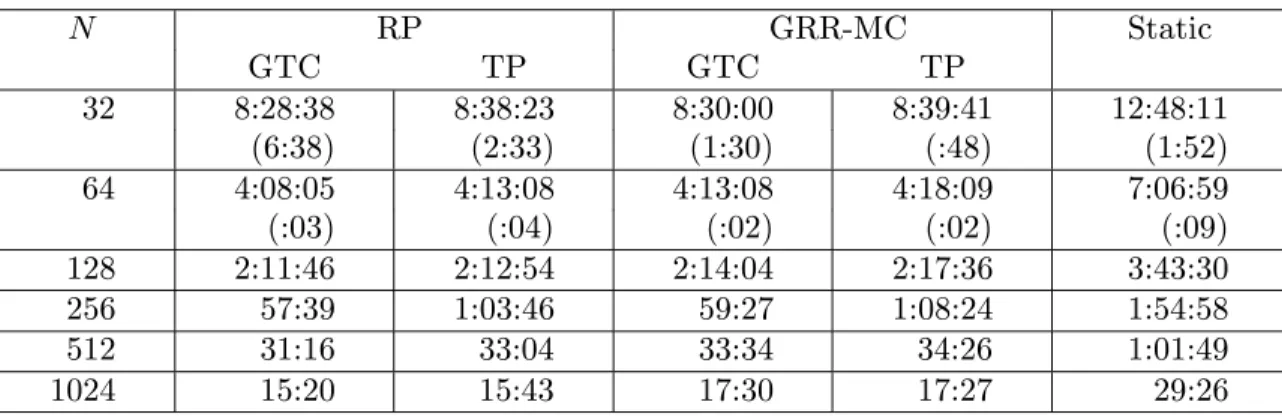
Table 3. Intel Paragon parallel times (hh:mm:ss) for low fidelity analysis of 2,026,231 HSCT designs. N RP GRR-MC Static GTC TP GTC TP 32 8:28:38 8:38:23 8:30:00 8:39:41 12:48:11 (6:38) (2:33) (1:30) (:48) (1:52) 64 4:08:05 4:13:08 4:13:08 4:18:09 7:06:59 (:03) (:04) (:02) (:02) (:09) 128 2:11:46 2:12:54 2:14:04 2:17:36 3:43:30 256 57:39 1:03:46 59:27 1:08:24 1:54:58 512 31:16 33:04 33:34 34:26 1:01:49 1024 15:20 15:43 17:30 17:27 29:26
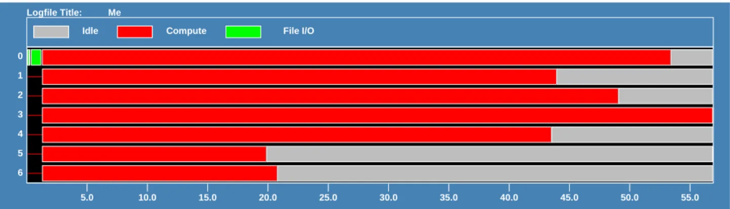
To test scalability and efficiency a relatively large data set with approximately 2 million (2,026,231) designs was generated using the point selection algorithm described earlier with order 4 and level 3. All runs have been performed on Intel Paragon platforms, which have a mesh architecture with Intel i860 XP processors comprising the computing entities. Figures 5–7 are snapshots produced with the nupshot utility, showing the states of nodes during execution for a small sample problem onN = 7 nodes. In these snapshots a processor can be in one of three states, performing useful computation, sitting idle, or reading initialization files—file I/O. When dynamic load balancing is not in effect (Figure 5), processors appear to spend half of their time being idle. With GRR-MC (Figure 6) and RP (Figure 7) idle states are more scattered, and seem significantly reduced. It can also be seen that even though RP and GRR-MC result in different distributions, both are very effective.
Table 3 shows execution times from the Intel Paragon computer XP/S 7 (100 compute nodes) at Virginia Tech, and the Intel Paragon XP/S 5, XP/S 35, and XP/S 150 (128, 512, 1024 compute nodes, respectively) computers at the Oak Ridge National Laboratory Center for Computational Sciences. Times are given in hours, minutes, and seconds; for
N ≤ 64 the average of five runs is reported, with the standard deviation in parentheses under the time. The same problem run on the XP/S 7 XP/S 5, and XP/S 35 Paragons takes
0 1 2 3 4 5 6 Logfile Title: Me
Idle Compute File I/O
5.0 10.0 15.0 20.0 25.0 30.0 35.0 40.0 45.0 50.0 55.0
Figure 5. Snapshot from nupshot utility of static load distribution,N = 7.
0 1 2 3 4 5 6 Logfile Title: Me
Idle Compute File I/O
5.0 10.0 15.0 20.0 25.0 30.0 35.0 40.0
Figure 6. Snapshot from nupshot utility of GRR-MC with global task count termination,N = 7. 0 1 2 3 4 5 6 Logfile Title: Me
Idle Compute File I/O
5.0 10.0 15.0 20.0 25.0 30.0 35.0 40.0
Figure 7. Snapshot from nupshot utility of RP with global task count termi-nation, N = 7.
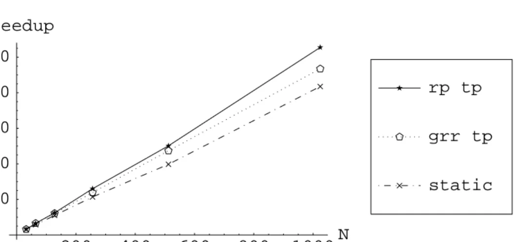
comparable amounts of time; times on the XP/S 150 Paragon tend to be a little higher (4 to 12 percent) than similar runs on the XP/S 35. Random polling uses the same fixed seed for all runs. For all other results,N ≥128, only one run was completed because of limited access to larger machines. The table starts from N = 32 nodes instead of N = 1 because the time required to run 2 million designs on one processor is prohibitive (>400 hours). Furthermore, the current implementation generates all the PBIB designs in one chunk, so the memory required (535 MBytes) for all designs would also be prohibitive. The original serial code has not been used for comparisons because its intensive use of file I/O makes it extremely inefficient, and thus infeasible even for problems of moderate size. Times in Table 3 do not include disk storage (1.2GBytes) for the final results. Figures 8 and 9 show speedup for all schemes, based on the execution times for N = 32 processors.
Several observations can be made from Figures 8–9 and Table 3.
(1) Scalability:all algorithms, including static distribution, scale well forN ≤1024 nodes, with random polling showing no noticeable degradation in efficiency atN = 1024 nodes. (2) Dynamic vs. static:both dynamic load balancing techniques seem to be very effective, 35 to 50 percent better than static distribution, and this difference increases with the number of processorsN.
(3) Stable execution times: the standard deviations of total execution time for runs on 32 and 64 processors are very small, which indicates that performance is relatively stable. Random polling is expected to have more variance in execution time when the seed is not fixed, but not a significant difference.
(4) Superlinear speedup: the latter rows of Table 3 exhibit superlinear speedup for global round robin with message combining and random polling. This implies that at 32 nodes the memory requirement (18 MBytes) for working with a relatively large number of tasks (≈63,319) per node can degrade performance on the XPS/7 platform due to resource starvation. See Quinn [26] for a discussion of general circumstances for superlinear speedup.
(5) Global task count vs. token passing:Global task count seems to outperform token passing for N ≤1024 with GRR-MC and RP, but the relative difference decreases for
200
400
600
800
1000
N
200
400
600
800
1000
speedup
static
grr gtc
rp gtc
Figure 8. Speedep with base N = 32 for RP and GRR-MC with global task count, on N = 2{5...10} processors.
200
400
600
800
1000
N
200
400
600
800
1000
speedup
static
grr tp
rp tp
Figure 9. Speedep with baseN = 32 for RP and GRR-MC with token passing, on N = 2{5...10} processors.
larger N. Clearly, the overhead involved in processing all completion messages (≥N) by one manager node under global task count increases withN.
(6) Random polling vs. global round robin with message combining: With both termination detection schemes random polling clearly outperforms global round robin with message combining. The relative difference in execution times increases as N
becomes larger. The simplicity of the random polling algorithm leads to the lack of any significant overhead. Contention conditions are unlikely to occur because messages are randomly directed and typically the number of unsuccessful work acquisition messages increases significantly only just before termination. Global round robin with message combining, on the other hand, involves a longer wait, comprised of a fair number of communication messages across the spanning tree, before it can send a work acquisition request and the price of unsuccessful work acquisition requests is higher, because they imply more time spent idle. Furthermore, on average the total number of messages processed by a node running GRR-MC is higher that that for a node running RP, since each request is propagated back and forth through as many as log2N other nodes. Finally, for both algorithms, the fact that all nodes start off with some load, which is expected to be relatively balanced among them for a large number of randomly long tasks, serves to decrease the initial number of unsuccessful work acquisition requests, which in turn improves performance.
7. PARAMETRIC STUDY.
The purpose of this study is to evaluate the effect, if any, of algorithmic parameters on the performance of the distributed schemes. Two dynamic load balancing parameters, splitting ratio and transfer threshold, discussed in Chapter 5.2, are reviewed, together with two algorithm-specific parameters, delaydfor GRR-MC and unsuccessful work acquisition attempts threshold U for token passing (TP). Delay is defined as CPU clock ticks, where the actual wait time is the delay clock ticks multiplied by the clock resolution. See Table 4 for the sets of values used to test these parameters. The variation of random polling times for five different seeds is also examined.
Table 4. Values for algorithmic parameters.
Parameter Set of Values
splitting ratioα {0.10,0.25,0.40,0.50,0.60,0.75,0.90} transfer threshold {0,15,30,45,60,75,90,105}
unsuccessful work acquisition attemptsU for TP {0,5,10,15,20,25}
delay dfor GRR-MC in clock ticks {500,1000,1500,2000,2500,3000,3500}
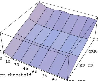
Comprehensive runs were initially performed with a relatively small data set of 30,915 configurations onN = 32 and 64 processors. A larger number of processorsN was not used because of time constraints on the larger Paragons. The trends observed were confirmed with a few runs on the large data set withN = 64 nodes. Both the delaydfor global round robin with message combining and the random seed for random polling introduced very small fluctuations in execution times—the variation was less than 1 percent in most cases. Variation of the unsuccessful acquisition attemptsU for token passing and the trans-fer threshold also resulted in a very insignificant diftrans-ference in execution time, and no particular pattern was observed. For instance, Figures 10 and 11 are surface plots show-ing how performance varies with different values for transfer threshold. The vertical axis denotes execution time in hours; the axis labeled transfer threshold is for the values
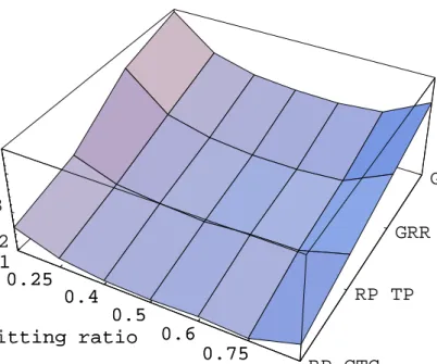
schemes RP GTC, RP TP, GRR-MC GTC, GRR-MC TP for which execution time is measured. Figures 12 and 13 are similar surface plots illustrating the effect of the splitting ratio α ∈ {0.10,0.25,0.40,0.50,0.60,0.75,0.90} parameter. A difference in time occurs at the two extreme values α ∈ {0.10,0.9}, and even here the increase in time is at most 15 percent. Runs on 64 nodes with the large data set of 2,026,231 configurations confirm the trend at the extreme values, but also show that the increase in time becomes less than 1 percent (see Figures 14 and 15).
0
15
30
45
60
75
90
105
transfer threshold
RP GTC
RP TP
GRR GTC
GRR TP
0.12
0.125
0.13
hours
0
15
30
45
60
75
90
er threshold
Figure 10. Effect of transfer threshold for N = 32 on 30,915 designs.
0
15
30
45
60
75
90
105
transfer threshold
RP GTC
RP TP
GRR GTC
GRR TP
0.065
0.07
hours
0
15
30
45
60
75
90
er threshold
0.1
0.25
0.4
0.5
0.6
0.75
0.9
splitting ratio
RP GTC
RP TP
GRR GTC
GRR TP
0.12
0.13
0.14
hours
1
0.25
0.4
0.5
0.6
0.75
itting ratio
Figure 12. Effect of splitting ratio α for N = 32 on 30,915 designs.
0.1
0.25
0.4
0.5
0.6
0.75
0.9
splitting ratio
RP GTC
RP TP
GRR GTC
GRR TP
0.065
0.07
0.075
0.08
hours
1
0.25
0.4
0.5
0.6
0.75
itting ratio
.1
.25
.4 .5 .6
.75
.9
splitting ratio
4.12
4.14
4.16
4.18
hours
Figure 14. Effect of splitting ratio on RP GTC forN = 64 on 2,026,23 designs.
15
30
45
60
75
90
transfer threshold
4.21
4.22
4.23
4.24
hours
8. CONCLUSIONS AND FUTURE WORK.
Distributed control and load balancing techniques were applied to an aspect of the multidisciplinary design optimization of a high speed civil transport. Two dynamic load balancing algorithms (random polling and global round robin with message combining) together with two necessary termination detection schemes (global task count and token passing) were implemented for the reasonable design space identification paradigm. Perfor-mance was evaluated on up to 1024 processors for all combinations of dynamic load balancing and termination detection schemes, plus the static distribution case. The effect of various algorithmic parameters was also explored, and found to be negligible except at extreme values. The results were very encouraging in terms of the effectiveness of dynamic load balancing (35–50 percent improvement over a static distribution), and the scalability of the algorithms (speedup was essentially linear). Most importantly, the time spent identifying the reasonable design space has been dramatically decreased, permitting the low fidelity analysis of 2 million designs, which was impractical before. The logical next step is to go beyond merely identifying the reasonable design space, and to identify good design regions within the reasonable design space, which would then be passed off to mildly parallel machines (e.g., IBM SP/2 or SGI Origin 2000) for “local” high fidelity optimization.
This effort is a stepping stone towards the goal of a MDO problem solving environment that will provide a complete and convenient computing environment for interactive multi-disciplinary aircraft design. As shown by the experience of Burgee et al. [7], Guruswamy [14], and many others, some crucial disciplinary analysis codes (for structural mechanics, fluid dynamics, aerodynamic analysis, propulsion, to name a few) perform very poorly in a multidisciplinary parallel computing environment. These codes represent hundreds of man-years of experience and development, and are unlikely to be rewritten for parallel machines any time soon. Thus the challenge is to find approaches to MDO (e.g., variable complexity modeling and response surface techniques) which permit the use of massively parallel computing for some phases of the process (one such phase was demonstrated here) and legacy disciplinary codes on serial computers for other phases. One highly touted solu-tion is “network computing”, but that still remains far from practical for serious large-scale multidisciplinary design.
REFERENCES.
[1] V. Balabanov, M. Kaufman, A.A. Giunta, B. Grossman, W.H. Mason, L.T. Watson, R.T. Haftka, “Developing customized weight function by structural optimization on parallel computers,” in 37th AIAA/ASME/ASCE/AHS/ASC, Structures, Structural Dynamics and Materials Conference, Salt Lake City, UT, pp. 113–125, Apr. 15-17 1996. [2] J.C. Becker, C.L. Bloebaum, “Distributed computing for multidisciplinary design opti-mization using Java,” inSixth AIAA/NASA/ISSMO Symposium on Multidisciplinary Analysis and Optimization, Bellevue, WA, pp. 1583–1593, Sept. 1996.
[3] C.H. Bischof, L.L. Green, K.J. Haigler, T.L. Knauff, Jr., “Parallel calculation of sensitivity derivatives for aircraft design using automatic differentiation,” in Fifth AIAA/USAF/NASA/OAI Symposium on Multidisciplinary Analysis and Optimiza-tion, Panama City, FL, pp. 73–86, Sept. 1994.
[4] G.E.P. Box, D.W. Behnken, “Some new three level designs for the study of quantitative variables,”Technometrics, vol. 2, 1960.
[5] R.D. Braun, I.M. Kroo, “Development and application of the collaborative optimization architecture in a multidisciplinary design environment,” inMultidisciplinary Design Op-timization: State of the Art, N. Alexandrov, M.Y. Hussaini (Eds.), SIAM, Philadelphia, PA, pp. 98–116, 1995.
[6] J. Brzezinski, J. H´elary, M. Raynal, “Distributed termination detection: General model and algorithms,” Tech. Rep. BROADCAST#TR93-05, ESPRIT Basic Research Project BROADCAST, Aug. 1993.
[7] S. Burgee, A.A. Giunta, V. Balabanov, B. Grossman, W.H. Mason, R. Narducci, R.T. Haftka, L.T. Watson, “A coarse-grained parallel variable-complexity multidisciplinary optimization paradigm,”The International Journal of Supercomputer Applications and High Performance Computing, vol. 10(4), pp. 269–299, 1996.
[8] J.E. Dennis, Jr., R. M. Lewis, “Problem formulations and other issues in multidisciplinary optimization,” Tech. Rep. CRPC-TR94469, CRPC, Rice University, Apr. 1994. [9] J.E. Dennis, Jr., V. Torczon, “Direct search methods on parallel machines,” SIAM
Journal of Optimization, vol. 1(4), pp. 448-474, Nov. 1991.
[10] D.J. Doorly, J. Peir´o, J.P. Oesterle, “Optimisation of aerodynamic and cou-pled aerodynamic-structural design using parallel genetic algorithms,” in Sixth AIAA/NASA/ISSMO Symposium on Multidisciplinary Analysis and Optimization, Bellevue, WA, pp. 401–409, Sept. 1996.
[11] M.S. Eldred, W.E. Hart, W.J. Bohnhoff, V.J. Romero, S.A. Hutchison, A.G. Salinger, “Utilizing object-oriented design to build advanced optimization strategies with generic implementation,” inSixth AIAA/NASA/ISSMO Symposium on Multidisciplinary Anal-ysis and Optimization, Bellevue, WA, pp. 1568–1582, Sept. 1996.
[12] O. Ghattas, C.E. Orozco, “A parallel reduced Hessian SQP method for shape opti-mization,” inMultidisciplinary Design Optimization: State of the Art, N. Alexandrov, M.Y. Hussaini (Eds.), SIAM, Philadelphia, PA, pp. 133-152, 1995.
[13] A.A. Guinta,Aircraft multidisciplinary design optimization using design of experiments theory and response surface modeling methods, Ph.D. dissertation, Department of Aerospace Engineering, Virginia Polytechnic Institute and State University, Blacksburg, VA, May 1997.
[14] G. Guruswamy, “Impact of parallel computing on high fidelity based multidisciplinary analysis,” in7th AIAA/USAF/NASA/ISSMO Symposium on Multidisciplinary Analysis and Optimization, St. Louis, MO, AIAA Paper 98-4709, pp. 67–80, Sept. 1998. [15] M.A. Hale, J.I. Craig, “Use of agents to implement an integrated computing
environ-ment,” in Computing in Aerospace 10, San Antonio, TX, AIAA Paper 95-1001, pp. 403-413, Mar. 1995.
[16] R.V. Harris Jr., “An analysis and correlation of aircraft wave drag,” NASA TM X-947 (1964).
[17] K.Hinkelman, Design and analysis of experiments, John Wiley & Sons, Inc., 1994. [18] D.A. Hopkins, S.N. Patnaik, L. Berke, “General-purpose optimization engine for
multi-disciplinary design applications,” in Sixth AIAA/NASA/ISSMO Symposium on Mul-tidisciplinary Analysis and Optimization, Bellevue, WA, pp. 1558–1565, Sept. 1996. [19] K. F. Hulme, C.L. Bloebaum, “Development of CASCADE: a multidisciplinary
de-sign test simulator,” in Sixth AIAA/NASA/ISSMO Symposium on Multidisciplinary Analysis and Optimization, Bellevue, WA, pp. 438–447, Sept. 1996.
[20] A. Jameson, J.J. Alonso, “Automatic aerodynamic optimization on distributed memory architectures,” in34th Aerospace Sciences Meeting and Exhibit, Reno, NV, AIAA Paper 96-0409, Jan. 1996.
[21] H. Kameda, J. Li, C. Kim, Y. Zhang,Optimal Load Balancing in Distributed Computer Systems, Springer-Verlag, 1997.
[22] M.D. Kaufman,Variable-complexity response surface approximations for wing structural weight in HSCT design, Master’s thesis, VPI and State University, Apr. 1996.
[23] D.L. Knill, A.A. Giunta, C.A. Baker, B. Grossman, W.H. Mason, R.T. Haftka, L.T. Watson, “Response surface models combining linear and euler aerodynamics for HSCT design,”Journal of Aircraft, to appear.
[24] I. Kroo, S. Altus, R. Braun, P. Gage, I. Sobieski, “Multidisciplinary optimization methods for aircraft preliminary design,” inFifth AIAA/USAF/NASA/OAI Symposium on Multidisciplinary Analysis and Optimization, Panama City, FL, pp. 697–707, Sept. 1994.
[25] V. Kumar, A.Y. Grama, V.N. Rao, “Scalable load balancing techniques for parallel computers,”Journal of Parallel and Distributed Computing, vol. 22(1), pp. 60–79, Jul. 1994.
[26] M.J. Quinn, Parallel computing : theory and practice, McGraw-Hill, New York, NY, 1994.
[27] S.A. Ridlon, “A software framework for enabling multidisciplinary analysis and opti-mization,” in Sixth AIAA/NASA/ISSMO Symposium on Multidisciplinary Analysis and Optimization, Bellevue, WA, pp. 1280–1285, Sept. 1996.
[28] P. Sanders, “A detailed analysis of random polling dynamic load balancing,” in Inter-national Symposium on Parallel Architectures, Algorithms, and Networks, Kanazawa, Japan, 1994, pp. 382–389.
[29] , “Some implementation results on random polling dynamic load balancing,” Tech. Rep. iratr-1995-40, Universit¨at Karlsruhe, Informatik f¨ur Ingenieure und Naturwis-senschaftler, 1995.
[30] M. Singhal, N.G. Shivaratri,Advanced Concepts in Operating Systems, McGraw-Hill, 1994.
[31] M. Snir, S. Otto, S. Huss-Lederman, D.W. Walker, J. Dongarra, MPI The Complete Reference, MIT Press, 1996.
[32] G. Tel, Topics in Distributed Algorithms, Cambridge International Series in Parallel Computation: 1, Cambridge University Press, 1991.
[33] , Introduction to Distributed Algorithms, Cambridge University Press, 1994. [34] R.P. Weston, J.C. Townsend, T.M. Edison, R.L. Gates, “A distributed computing
envi-ronment for multidisciplinary design,” in Fifth AIAA/USAF/NASA/OAI Symposium on Multidisciplinary Analysis and Optimization, Panama City, FL, pp. 1091–1095, Sept. 1994.
[35] B.A. Wujek, J.A. Renaud, S. M. Batill, “A concurrent engineering approach for mul-tidisciplinary design in a distributed computing environment,” in Multidisciplinary Design Optimization: State of the Art, N. Alexandrov, M.Y. Hussaini (Eds.), SIAM, Philadelphia, PA, pp. 189–208, 1995.
[36] S. Yoder, J. Brockman, “A software architecture for collaborative development and solution of MDO problems,” in Sixth AIAA/NASA/ISSMO Symposium on Multidis-ciplinary Analysis and Optimization, Bellevue, WA, pp. 1060–1062, Sept. 1996.
Appendix A: CODE FOR MESSAGE PROCESSING THREAD.
TheCcode where all threads are invoked and message handling takes place, as mentioned in Chapter 4.1.2., is listed in this appendix.
#include <stdio.h> #include <stdlib.h> #include <pthread.h> #include <mpi.h>
#include "prof.h" /** profiling constants **/
#include "defines.h" /** const definitions for structs.h **/ #include "structs.h" /** aircraft struct definition **/ #include "HSCTSearch.h"
#include "lib.h" /** matrix functions **/ #include "prelim.h" #include "compute.h" #include "grr_mc.h" #include "random.h" #include "worker.h" #include "safemem.h" #define COMM_BUFS 10 /**
Token Passing variables that are shared between the worker thread, the token passing routine, and the message handling routine **/
int idle, token_count_buf, token_received, unsucc_work_attempts, expecting_reply; /************************************************************************************* ComputationPhase: Routine for message processing; it starts off the other
threads respective of the algorithm parameters passed by the user. The main part of this routine consists of a loop that checks for messages and processes them.
**************************************************************************************/ int ComputationPhase( struct cntrl_struct *cntrl, MatrixClass *dvar,
MatrixClass *local_points, Aircraft *aircraft, Prog_Args_Struct *prog_args_struct)
{
register int i;
int my_rank, group_size, done_count, carryover, error_status, j, num_leaves, num_leaves_rcvd, child_leaves, child, index, target_node, test_flag, tot_sent_work, tot_work_rcvd, tot_work_rcvd_buf, total_msgs, tot_sent_work_buf[COMM_BUFS],
*grr_msg_buf = NULL, *done_indices = NULL; double dbl_work_sent,
*work_rcvd_buf = NULL, *work_sent = NULL; Q_Element *q_el = NULL;
MPI_Request rqst_work_rqst= MPI_REQUEST_NULL,
rqst_work_sent[COMM_BUFS], rqst_qty_work_sent[COMM_BUFS], *mpi_rqst = NULL;
MPI_Status work_sent_status, work_rqst_status, terminate_status, carryover_status, *mpi_status = NULL;
Worker_Args_Struct worker_args; GRR_MC_Args_Struct grr_mc_args; MPI_Datatype MPI_MATRIX_ROW;
pthread_t thread_id[TOTAL_THREADS];
/** Global task count termination variables **/ int buf_tasks_cmplt = 0, tasks_cmplt_count = 0 ; /** GRR - MC variables **/
int **msg = NULL, *data = NULL;
MPI_Comm_size( MPI_COMM_WORLD, &group_size); MPI_Comm_rank( MPI_COMM_WORLD, &my_rank); error_status = PRELIM_SUCCESS;
MPI_Type_contiguous( local_points->nDim+1, MPI_DOUBLE, &MPI_MATRIX_ROW); MPI_Type_commit( &MPI_MATRIX_ROW );
/** initialization of global shared variables **/
pthread_mutex_init(&mutex_matrix, pthread_mutexattr_default); pthread_cond_init(&cond_worker_wait, pthread_condattr_default); tasks_matrix.nDim = local_points->nDim; tasks_matrix.mDim = local_points->mDim; tasks_matrix.d = local_points->d; matrix_cur_pos = 1; matrix_top_pos = local_points->mDim; dlb = FALSE; termination = FALSE; total_msgs = TOT_MAIN_MSG_TYPES; /** TOKEN TERMINATION **/ if (prog_args_struct->TERM == TERM_TOKEN) { expecting_reply = FALSE; unsucc_work_attempts = 0; if ((matrix_top_pos-matrix_cur_pos)+1 > 0) idle = FALSE; else idle = TRUE; token_count_buf = 0; if ( my_rank == MASTER_RANK) token_received = TRUE; else token_received = FALSE; }
/** GRR-MC **/
if (prog_args_struct->D_L_B == D_L_B_GRR_MC) {
total_msgs += GetGRRMessageCount(my_rank, group_size); msg = MsgIntBufferCreate(my_rank,
total_msgs-TOT_MAIN_MSG_TYPES, GRR_MC_MSG_SIZE); grr_msg_buf = safe_malloc(GRR_MC_MSG_SIZE*sizeof(int)); if ( grr_msg_buf == NULL)
{
fprintf(stderr, "worker(%d): cannot allocate grr_msg_buf!\n",my_rank); return PRELIM_ERROR;
} }
/** RANDOM_POLLING **/
else if (prog_args_struct->D_L_B == D_L_B_RANDOM_POLLING) {
Init_Random_Polling(group_size,
(unsigned int) prog_args_struct->RANDOM_SEED *my_rank); }
/** allocation of MPI request handles for the persistent recieves **/ mpi_rqst = (MPI_Request *) safe_calloc( total_msgs, sizeof(MPI_Request)); if ( mpi_rqst == NULL )
{
fprintf(stderr, "ComputationPhase(%d): cannot allocate mpi_rqst!\n", my_rank);
return PRELIM_ERROR; }
/** allocation of MPI structures for storing the status of persistent receive requests **/
mpi_status = (MPI_Status *) safe_calloc( total_msgs, sizeof(MPI_Status)); if ( mpi_status == NULL )
{
fprintf(stderr, "ComputationPhase(%d): cannot allocate mpi_status!\n", my_rank); return PRELIM_ERROR;
}
done_indices= (int *) safe_calloc( total_msgs, sizeof(int)); if ( done_indices == NULL )
{
fprintf(stderr, "ComputationPhase(%d): cannot allocate done_indices!\n", my_rank); return PRELIM_ERROR;
}
/** reset MPI request handles to NULL **/ for ( i = 0; i < total_msgs; i++ )
mpi_rqst[i] = MPI_REQUEST_NULL; for ( i = 0; i < COMM_BUFS; i++ ) {
rqst_work_sent[i] = MPI_REQUEST_NULL; work_sent_buf[i] = NULL; rqst_qty_work_sent[i] = MPI_REQUEST_NULL; } /** creation of GRR-MC thread **/ if (prog_args_struct->D_L_B == D_L_B_GRR_MC) { /** create GRR-MC threads **/ grr_mc_args.grr_mc_delay = prog_args_struct->grr_mc_delay; pthread_create(&thread_id[DLB_THREAD], pthread_attr_default,
(void *)GRR_MC_Routine, (void *)&grr_mc_args); pthread_yield();
pthread_yield(); }
/** creation of worker thread **/
worker_args.cntrl = (struct cntrl_struct *) cntrl; worker_args.dvar = (MatrixClass *) dvar;
worker_args.aircraft = (Aircraft *) aircraft;
worker_args.prog_args_struct = (Prog_Args_Struct *)prog_args_struct; pthread_create(&thread_id[WORKER_THR