PIPE BURST DIAGNOSTICS USING EVIDENCE THEORY

PIPE BURST DIAGNOSTICS USING EVIDENCE THEORY

JOSEF BICIK1, ZORAN KAPELAN1, CHRISTOS MAKROPOULOS2 & DRAGAN A. SAVIĆ1

1 _{Centre for Water Systems, School of Engineering, Mathematics and Physical Sciences, University of}

Exeter, North Park Road, Exeter, Devon, EX4 4QF, United Kingdom, E-mail: {j.bicik, z.kapelan, d.savic}@exeter.ac.uk, Tel.: +44 1392 723730, Fax: +44 1392 217965

2 _{School of Civil Engineering, National Technical University of Athens, Heroon Polytechneiou 5, Athens,}

GR-157 80 Greece, E-mail: [email protected], Tel.: +30 210 772 2886

Abstract

This paper presents a decision support methodology aimed at assisting Water Distribution System (WDS) operators in the timely location of pipe bursts. This will enable them to react more systematically and promptly. The information gathered from various data sources to help locate where a pipe burst might have occurred is frequently conflicting and imperfect. The methodology developed in this paper deals effectively with such information sources. The raw data collected in the field is first processed by means of several models, namely the pipe burst prediction model, the hydraulic model and the customer contacts model. The Dempster-Shafer Theory of Evidence is then used to combine the outputs of these models with the aim of increasing the certainty of

applied to several semi-real case studies. The results obtained demonstrate that the method is capable of locating the area of a pipe burst by capturing the varying credibility of the individual models based on their historical performance.

Keywords: decision support, diagnostics, evidence theory, pipe burst, water distribution system.

NOTATION

Θ frame of discernment

m() basic probability assignment

Bel Belief function

Pl Plausibility function

BetP Pignistic probability function

K conflicting probability mass

INTRODUCTION

The operation of Water Distribution Systems (WDS) is a complex process relying on the experience of operators who often have to base their decisions on scarce and incomplete information. Under normal operating conditions the behaviour of WDS is understood relatively well and can be simulated using hydraulic models. However, when pipe bursts occur, the lack of information makes the diagnostics task difficult. Pipe bursts cause water and energy losses (Colombo & Karney 2002), and can also lead to flooding of properties (Cooper et al. 2000) and intrusion of contaminants into the WDS (Sadiq et al.

2006). Timely detection and location of pipe bursts is therefore of primary interest to water utilities worldwide in order to improve their customer service, minimise leakage, preserve resources and thus minimise impact on the environment.

Pipe burst prediction models have been developed in order to model the deterioration of underground assets (Kleiner & Rajani 2001). However, such models are more suitable for strategic planning and cannot be utilised on their own to support operational decisions, e.g., to locate a pipe burst in the system in real-time. With recent advances in sensor technologies, “intelligent”, wireless and inexpensive pressure and flow sensors have been widely deployed to monitor the state of the WDS in real-time. Their data have been used in combination with model-based methodologies attempting to detect and locate leakage or pipe bursts within a WDS. Andersen & Powell (2000) presented an implicit state estimation technique to locate a burst and demonstrated the methodology on a simple looped network without explicitly taking into account uncertainty and measurement errors. Poulakis et al. (2003) developed a Bayesian probabilistic framework for pipe burst detection and showed the capability of the methodology to identify the most likely burst location on a synthetic case study. Wu et al. (2008) used genetic algorithms to optimise the pressure-dependent emitter locations and coefficients as possible leakage and illustrated the methodology on a real-life network. Misiunas et al. (2006) used the EPANET (Rossman 2000) hydraulic solver to find a burst location by comparing the fit between the modelled and measured pressures in a WDS. Despite the progress achieved there is little evidence that these methods, when used on their own, are ready to be applied in real-life conditions for near real-time decision support of WDS operation.

In this paper, a methodology for combining the outputs of several models (including a Pipe Burst Prediction Model (PBPM), a Hydraulic Model (HM) and a Customer Contacts Model (CCM)) is proposed, to improve the potential for reliable and rapid identification of the possible locations of a pipe burst. This is essential to water companies, reflecting a proactive approach that attempts to detect and resolve failures in the WDS before they start affecting customers. This is not always possible and in some situations the water company reacts only after a problem is first reported by customers. In the proposed methodology, information provided by individual models is fused together, using the Dempster-Shafer (D-S) theory of Evidence (Shafer 1976). The combined output, which encapsulates the varying credibility of the individual models, provides the spatial

distribution of Belief and Plausibility (e.g., Figure 4e and Figure 4f) of failure of any pipe in the studied WDS to support the decision making process by an operator. This

evidential reasoning approach further reduces the information load faced by operators and increases confidence in the results that are supported by several models.

DEMPSTER-SHAFER THEORY

The D-S theory, also known as Evidence Theory, was first formulated in the late 1970’s by Dempster (1967) and later on extended and formalised by Shafer (1976). D-S theory can be used for inference in the presence of incomplete and uncertain information, provided by different, independent, sources. A significant advantage of D-S theory is its ability to deal with missing information and to estimate the imprecision and conflict between different information sources.

Sentz & Ferson (2002) provided a review of applications of D-S theory in various disciplines including classification and recognition, decision making, engineering and optimization, fault detection and failure diagnostics, etc. Evidence theory has also been used in water related applications. Démotier et al. (2003) applied D-S theory to risk analysis of water treatment processes. Sadiq and Rodriguez (2005) and Sadiq et al.

(2006) used D-S theory to interpret water quality data. Li (2007) used D-S theory to aggregate risk levels in a hierarchical risk assessment of components, subsystems, and the overall water supply system. Bai et al. (2008) used Dempster’s combination rule in a hierarchical aggregation of evidence for condition assessment of buried pipes.

The D-S theory operates on a “frame of discernment” Θ, which is a finite set of mutually exclusive and exhaustive propositions. Unlike traditional Bayesian models (Bayes 1763), probability mass can be assigned to subsets of the frame of discernment Θ using a Basic Probability Assignment (BPA), typically denoted m(A), where A is a non-empty subset of Θ. D-S theory defines two fundamental functions: Belief (Bel) and Plausibility (Pl):

∑

∑

where: B is a non-empty subset of Θ.

Bel corresponds to the total mass of evidence, which supports a proposition and all of its subsets, whereas Pl corresponds to the total mass of evidence, which is not in

In this study, a Binary Frame of Discernment (BFOD) Θ (Safranek et al. 1990), is used, comprising two propositions (“Burst” and “NoBurst”) representing the likelihood of occurrence / non-occurrence of a burst. The power set 2Θ is thus formed by the following subsets: (Ø,{Burst},{NoBurst},{Burst, NoBurst}), where the subset {Burst, NoBurst} represents the whole frame of discernment Θ and any probability mass assigned to this subset corresponds to a lack of knowledge (i.e., ignorance). The chosen definition of the BFOD implies that the process of identifying the location of a burst pipe is similar to a classification problem where a value of belief is calculated for every pipe in the WDS indicating the likelihood of that pipe being the true (i.e., {Burst}) or false (i.e.,

{NoBurst}) burst location.

Dempster’s rule of combination (Shafer 1976) is an inherent part of D-S theory which allows combining information from different, independent sources of evidence. It is defined as follows: 0 1 ) ( ) ( ) ( 2 1 2 , 1 ≠ / − =

∑

∑

where: m1,2 is the combined BPA, m1, m2 are the BPAs of independent sources of

evidence, K represents the level of conflict amongst the evidence and A, B and C are non-empty subsets of Θ.

Since the introduction of Dempster’s rule various other combination rules have been developed (Sentz & Ferson 2002). In this work, Yager’s combination rule (Yager 1987) and the PCR5 combination rule (Smarandache & Dezert 2006) were used, in addition to Dempster’s rule, to observe their different behaviour and performance in the process of information fusion. These rules differ in the way they distribute conflicting probability mass K amongst the propositions of Θ. Dempster’s rule distributes the conflicting mass equally amongst all propositions of Θ, Yager’s rule attributes all conflicting mass to Θ and the PCR5 rule proportionally redistributes partial conflicting masses amongst propositions involved in the partial conflict.

To make decisions based on belief functions, Smets & Kennes (1994), proposed a model of transformation, based on the assumption that “beliefs manifest themselves at two mental levels: the ‘credal’ level where beliefs are entertained and the ‘pignistic’ level where beliefs are used to make decisions”. Based on the principle of insufficient reason, Smets & Kennes (1994) defined the pignistic probability function BetP as follows:

2 ( ) ( ) A B A BetP B m A A Θ ∈ ∩ =

_∑

The pignistic probability function (BetP) is a measure that can be used to present the outputs of the information fusion process to the decision maker and will be later utilised in performance evaluation of the information fusion methodology.

INFORMATION SOURCES

Due to the flexibility of D-S theory, any kind of information providing an indication of the likelihood of a particular pipe bursting in the WDS can be combined to reduce the

lack of knowledge about the location of the failed pipe and increase the confidence in its correct identification. This research utilises three information sources that are considered to be independent: (a) a PBPM output, (b) a CCM output and (c) a HM output. As discussed by Marashi et al. (2008) and Bi et al. (2008) the assumption of their

independence is realistic. This particular set of information sources was chosen because of its general availability to many water utilities worldwide and does not prevent other information sources from being used (see conclusions for examples). The first source of information (i.e., based on the pipe burst prediction model output) is treated as a static indicator of pipe burst occurrence whereas the other two remaining sources can be dynamic and provide new information as it becomes available (e.g., when another customer complaint is received or when the HM is updated with new real-time measurements obtained from field sensors).

Pipe Burst Prediction Model

A regression-based PBPM is used to obtain expected burst frequencies for every pipe in the studied WDS during the current month. The burst frequency of a pipe is expressed as a function of its material, diameter, age, soil type, land use and weather conditions. The specific expression and the related coefficients used in this work can be found in (Tynemarch Systems Engineering Ltd. 2007) and will not be reported here as it falls outside the scope of this paper.

The current methods of detection and location of pipe bursts aim to notify the control room personnel of any abnormal conditions before a failure starts affecting customers. However, frequently, large pipe bursts are first reported by customers (i.e., when leaked water emerges on the surface or when a partial/full interruption to supply is noticed). In situations where no explicit pipe burst detection mechanisms are in place, customer reports are the only means of (reactive) response to control leakage. Despite being a very strong indicator of a burst location, customer contacts are imperfect and cannot be entirely trusted. A CCM was developed under the assumption that customers typically report pipe bursts in the proximity of where they live. The coordinates of the property (i.e., easting and northing) from which a customer contact originated, were used in this work. Furthermore, the CCM used a weighted distance to reduce the influence of outliers (i.e., misleading customer contacts) in situations when multiple customer contacts were received. The mathematical formulation of the model is as follows:

, min( ) i _j i j j CCM = d ×w ₍₇₎

(

)

(

)

∑

where: i is the index of a pipe, di,j is the (shortest) distance between pipe i and customer

contact j (CCj), wj is a weight reflecting the significance of a particular customer contact

(i.e., the lower the value of wj the more significant a given customer contact is), NCC is

the total number of customer contacts associated with a particular pipe burst and C is the centroid of all customer contacts related to the pipe burst.

A HM was used to locate a burst in a WDS by simulating its effects (i.e., an increase in flow and drop in pressure) and compare them with values obtained from pressure and flow sensors deployed in the field. An estimated magnitude of the burst flow is first provided by a detection system able to discover abnormally high inflows into a District Metered Area (DMA) (Mounce & Machell 2006; Romano et al. 2009). An extra demand, equal to the estimated burst flow, is then added to the centre of every pipe to model the effects of a burst in that location. The pressure boundary conditions of the HM are set according to the data obtained from inlet pressure sensors at the time when the burst was first detected. The customer demands are proportionally scaled so that they add up to the measured inflow into the DMA obtained from the DMA inlet flow meters data (i.e., customer demands = DMA inflow - burst flow). The likelihood of any pipe bursting in the system is then indicated by a sum of squared errors between observed and modelled pressures calculated as follows:

2 1, 2, 1 1 ( ( ) ( )) S N T i s s s t HM P t P t = = =

∑∑

where: i is an index of the burst pipe in the HM, s is an index of a node where a pressure sensor is located, NS is the total number of pressure sensors in the network, T is the

number of pressure measurements available (i.e., different times), P1,s(t) is the modelled

pressure at time t at node s and P2,s(t) is the measured pressure at time t at node s. Flow

measurements inside a DMA were not utilised since these are not typically available in real-life systems (at least not in the UK) due to the higher cost of flow meters in comparison to pressure sensors.

Each of the information sources described above provides a single output (i.e., criterion measurement) for each pipe in the WDS reflecting the likelihood (i.e., a normalised value of the criterion measurement) of occurrence of a burst on that pipe. The individual

information sources used are not considered to be fully reliable and each may be

associated with a different level of credibility. In order to improve combined confidence in the location of a pipe burst, the information from all available sources is fused using the D-S theory by applying a suitable combination rule.

Before the outputs of individual models can be combined, the criterion measurements need to be transformed into BPAs, each representing the exact belief in the given proposition (i.e., {Burst}, {NoBurst}) as well as the degree of ignorance (i.e., {Burst,

NoBurst}). For this purpose a two-step procedure was adapted from Beynon (2005). The criterion measurement values are first converted to confidence factors using a suitable normalisation function and then transformed into BPAs as shown in Figure 1.

The ideal position of Figure 1

Beynon (2005) used a sigmoid normalisation function to transform criterion measurements into confidence factors that were mapped to corresponding BPAs. Similarly to Safranek et al. (1990), Beynon (2005) applied simple symmetric functions defined by two parameters A and B to map confidence factors to BPAs. On the other hand, Sadiq et al. (2006) used trapezoids, typical for fuzzy sets, to obtain BPAs directly from criterion measurements. In this work, however, the type of normalisation functions (i.e., linear, sigmoid, one-sided Gaussian and logit function) as well as the shape of the

mapping functions (defined by 8 parameters, i.e., 4 points A1, B1, A2 and B2 as shown in

Figure 1) were determined for each of the input models based on its historical

performance. The mapping function describing m({Burst}) is a non-decreasing function whereas the function describing m({NoBurst}) is a non-increasing function. Once the evidence for every pipe in the network is transformed to BPAs the individual pieces can be combined using a combination rule. The actual rule used is determined as part of a calibration procedure so that the ensemble of the combination rule, the normalisation and mapping functions gained the maximum benefit according to the criteria outlined in the results and discussion section.

CASE STUDY

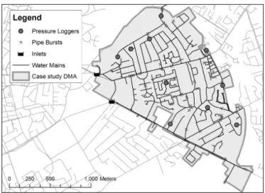
The proposed methodology was applied to a case study based on data from a real system in North Yorkshire, UK. The studied DMA (see Figure 2) was an urban, highly looped network with 2 inlets and no exports, supplying water to over 4,500 customers.

The ideal position of Figure 2

The available dataset contained information about main repairs from a Work

Management System (WMS), customer contact data and asset data providing required inputs into the PBPM. In order to calibrate the D-S model it was necessary to obtain details about a number of historical pipe bursts. During the period from April 2002 to April 2008 54 pipe bursts were recorded in this DMA at locations shown in Figure 2. Customers reported 65% of the pipe bursts either 24 hours before the burst was repaired

or during the same day when the repair took place. Based on this, it was assumed here that a burst pipe was repaired the same day that an anomaly was detected. The time window over which customer contacts were considered to be related to a particular burst event was established by performing spatial analysis of customer contacts and WMS data of a large number of DMAs. The size of the window was chosen as the best trade-off maximising the number of customer contacts associated with pipe bursts and minimising the distance of those contacts from the location of the burst pipe.

The use of the HM as a source of evidence required a relatively high number of pressure sensors in the network depending on its size and topology in order to achieve acceptable performance. Water companies in the UK typically do not monitor pressure at sufficient number of locations in the WDS. Ten pressure sensors were deployed in the case study area in 2009 at locations indicated in Figure 2. However, throughout the period from 2002 until 2008 pressure and flow data were not collected in sufficient quantity, nor was an online pipe burst detection system (Mounce et al. 2009), capable of providing

estimates of the abnormal burst flows, in place. Therefore the inputs into the HM (i.e., pressure and flow measurements and estimated burst flow magnitude) had to be synthetically generated. A large burst (between 4.5 and 5.5 l/s, i.e., around 15% of the peak demand) was first simulated as a fixed demand added to the centre of a pipe nearest to the location obtained from the WMS system. Pressures in the system obtained at demand nodes closest to the real location of sensors, were recorded and used as reference pressures representing a pipe burst situation. Uniformly distributed noise of 2% and 7.5% was added to the reference pressures and nodal demands, respectively, to reflect real-life

conditions more closely. These figures are representative of the pressure sensors used and real-life demand conditions in the DMA. Without adding any noise the HM would always find the right location of the burst and would significantly outperform the remaining information sources. It was assumed that the magnitude of the burst flow was known and no noise was added to this input parameter at this stage.

The complete dataset comprising 54 historical pipe bursts was split into a calibration set comprising 41 cases and a validation set comprising 13 cases (approx. ratio 75%

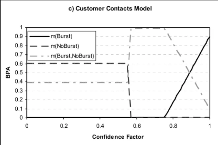
calibration / 25% validation). The split between calibration and validation data was done in such a way that both datasets had similar properties (e.g., in terms of number of customer contacts received and the performance of individual models). The calibration procedure aimed to determine the most suitable normalisation and mapping functions as well as the combination rule that would produce the best combined results. The resulting mapping function of the CCM tailored specifically for the case study DMA is shown in Figure 3 as an example. The most suitable normalisation function for the PBPM was the sigmoid function and for the HM and the CCM, was the logit function. Dempster’s rule yielded better results in view of the calibration objectives than Yager’s and the PCR5 combination rules. Note that the above findings should be considered case specific and should not be generalised in other situations. The same methodology can, however, be used in other cases to identify appropriate normalisation functions and combination rules.

As can be seen from Figure 3, the mapping function captures different behaviour of the analysed model. In the case of the CCM, it can be observed that in a high number of cases customers reporting a burst were located in close proximity to the pipe burst. However, a portion of customer contacts was misleading, which explains the shape of the mapping function in Figure 3.

RESULTS AND DISCUSSION

The main aim of information fusion applied in the context of pipe burst diagnostics is to identify hotspots, comprising a small number of pipes, where the burst is most likely to be located. Figure 4 illustrates the performance of the D-S model on a historical pipe burst selected from the validation dataset. In this case, the burst was reported by two customers and therefore all three sources of evidence were available.

The ideal position of Figure 4

The accuracy of the PBPM was limited and a large number of pipes received the same confidence factor (see Figure 4a). The HM performed poorly in this particular case and identified two possible pipe burst hotspots, with the most likely location being far from the burst pipe (see Figure 4b). One of the customer contacts was received from a location in close proximity to the burst pipe whereas the other one was more than 250m away from the burst location (see Figure 4c). Based on the input of the CCM, the D-S model attributed higher levels of BetP(Burst) to the pipes in the second pipe burst hotspot previously identified by the HM, supporting the proposition that this was the true location of the burst (see Figure 4d). The pipes close to the second customer contact, which was

further away from the true location of the burst, received a lower level of BetP(Burst). Therefore a field investigation, based on the results of the D-S model, would focus on the first customer contact and thus reduce the time for repair, reducing the amount of water lost from the system and the possible follow-on (socio-economic) impact on customers.

Performance comparison

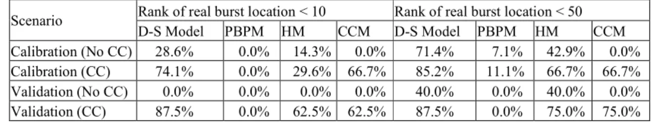
Table 1 shows the performance of the D-S model and of the individual models both on calibration and validation cases. These were further split depending on the presence of customer contacts (CC). The comparison was based on the ranking of the real burst pipe according to the output of the D-S model (i.e., the BetP(Burst)) and the ranking assigned by individual models (i.e., criterion measurements). The performance of any model was considered good if the real burst location was among the top 10 burst candidates

identified by the respective model. As can be seen from Table 1 none of the individual input models, i.e., the PBPM, HM and CCM, was able to achieve the above goal in all of the situations (i.e., 54 historical pipe bursts) considered in the case study. The degree of success in identifying the location of a burst pipe varied significantly amongst the models. According to this assessment criterion the overall performance of the D-S model was on average in every scenario either equally good or better than any of the individual models. Similar performance can be observed in Table 1 where the number of potential burst candidates was increased from 10 to 50.

Evaluating the benefits of information fusion algorithms is not simple and using only the measure above would not reflect the additional advantages of this approach. A particular model might fail to identify the correct burst location according to the criteria used above but can, on the other hand, still identify a number of locations where the burst pipe is unlikely to be located. To take this fact into the account and to compare the quality of the output of the D-S model and the individual models, the following set of performance indicators was established:

1. Likelihood concentration. For the method to be useful operationally, it is important that the likelihood of burst occurrence assigned to the pipes near the real burst location is higher than the likelihood assigned to pipes further away. This can be expressed using the ratio of the average likelihood of occurrence of the burst assigned to pipes close to the true burst location over the average likelihood of burst occurrence assigned to all remaining pipes. The higher this ratio is, the better the overall performance of a particular model. The set of pipes in the proximity of the true burst location was assumed here as the 10

topologically nearest pipes. Given that the average length of the pipes in the case study area was 30m and that the network was highly looped, such resolution should be considered acceptable.

2. Certainty. According to Yager (2004), Shannon entropy (Shannon 1948) was used to characterise the certainty of the outputs of the individual models and the D-S model. The entropy of an information source (i.e., output of a particular model)

was calculated using Eq. (10) and its certainty can be expressed using Eq. (11). The higher the certainty of a particular model the better was its performance.

1 ( ) ln( ( )) P N k k k H p Burst p Burst = = −

∑

where: H is Shannon entropy, pk is either the normalised BetPk(Burst) or the

normalised value of confidence factor of a potential incident (pipe) k in the case of the D-S model and the individual models, respectively and NP is the number of

potential incidents (i.e., pipes) in the system

The results of the comparison based on the two additional criteria suggested above are shown in Table 2, which indicates in how many calibration and validation cases was the D-S model better than the individual models (values above 50% indicate that the D-S model on average improved over the prediction of an individual model and 100% means that the D-S model was better in all considered cases than a particular individual model). Again, cases are further split into scenarios where customer contacts were and were not available.

The ideal position of Table 2

As it can be seen from Table 2, the D-S model yields better results in terms of the

Likelihood concentration in a higher number of cases compared to the individual models. The D-S model was significantly better than the PBPM and CCM in view of the

fact is most apparent in scenarios where no customer contacts were received and only the outputs of the HM and PBPM were combined. In such situation the most likely locations of the burst pipe typically form a number of scattered hotspots rather than a relatively well confined area as shown in Figure 4d. Despite this fact the use of the PBPM as an information source still yields certain benefits as illustrated in Table 1.

Sensitivity analysis

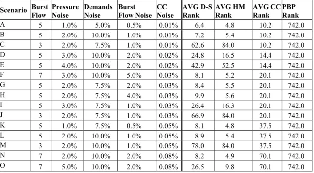
To investigate the sensitivity of individual model outputs as well as the D-S model output to the noisy inputs, global sensitivity analysis using Monte Carlo simulation (1,000 samples) was performed on the example presented in Figure 4. The selected case represented a suitable scenario from the validation data set since at least two of the individual models (i.e., the HM and the CCM) performed acceptably and therefore the effect of the added noise could be observed. Various levels of uniformly distributed noise as indicated in Table 3 were added to the inputs of the individual models, namely the HM (observed pressures, demands and estimated burst flow) and the CCM (Easting and Northing). Adding noise to the PBPM would be problematic and given its relatively low credibility it would not make a significant difference in this case.

The ideal position of Table 3

As can be seen from Table 3 the combined results are to some extent less sensitive to the noise added to the inputs of individual models. If the performance of only one of the models degrades significantly, the two remaining models (the CCM in particular) would still influence the combined results so that they did not degrade as fast as the worst

model. However, in cases where the amount of noise added to both input models (i.e., the HM and the CCM) at the same time exceeded reasonable thresholds (e.g., Scenario D and I in Table 3), far from what was present in the calibration dataset, then the combined results were, in a small number of cases, worse than those of any of the two key input models.

CONCLUSIONS

Locating a pipe burst within a DMA using data driven or conventional model-based methods is a challenging problem. The main constraint of such methods is typically the lack of data or insufficient calibration of the models used. Under such conditions of uncertainty, when no single model is able to provide a satisfactory answer, it is beneficial to combine the outputs from several models, based on different inputs, in order to

improve confidence in the overall result. This paper presents a methodology based on D-S Theory which combines evidence from several independent sources/models (i.e., a pipe burst prediction model, a hydraulic model and a customer contacts model) to locate a pipe burst within a DMA. It is argued that this methodology is able to fully exploit all information sources available in a WDS Control Room and reduce the information load that needs to be processed by a human operator.

A limiting factor to a wider application of hydraulic models in near real-time burst diagnostics is the unavailability of pressure and flow data in sufficient quantity and quality. Water utilities in the UK have only recently started to collect such data and even now it is still difficult to find a sufficient number of pressure monitoring points. The lack

of field data prevented the application of the methodology to a real-life system. The results obtained on a number of semi-real historical pipe bursts suggest that the method (depending on the quality of the input evidence) is capable of identifying the most likely area of the pipe burst. The methodology has the potential to learn from the performance of individual models during the calibration stage and successfully apply this knowledge to unseen cases. When feedback about new pipe bursts becomes available, the D-S model can be recalibrated in order to better reflect the evolving performance of the input

models. Moreover, additional models suggesting the location of a burst pipe (e.g., based on the information of third parties working in the system, weather information, etc.) can be incorporated as additional information sources, to further improve the benefits of information fusion.

ACKNOWLEDGMENTS

The work on the NEPTUNE project was supported by the U.K. Science and Engineering Research Council, grant EP/E003192/1, and Industrial Collaborators. In particular, the authors would like to express their gratitude to Mr. Ridwan Patel from Yorkshire Water Services and Dr. Steve Mounce from the Pennine Water Group for their kind assistance.

REFERENCES

Andersen, J. H., & Powell, R. S. 2000 Implicit state-estimation technique for water network monitoring. Urban Water, 2(2), 123-130.

Bai, H., Sadiq, R., Najjaran, H., & Rajani, B. 2008 Condition Assessment of Buried Pipes Using Hierarchical Evidential Reasoning Model. Journal of Computing in Civil

Engineering, 22(2), 114-122.

Bayes, T. 1763 An essay towards solving a problem in the doctrine of chances.

Beynon, M. J. 2005 A novel technique of object ranking and classification under ignorance: An application to the corporate failure risk problem. European Journal of Operational Research, 167(2), 493-517.

Bi, Y., Guan, J., & Bell, D. 2008 The combination of multiple classifiers using an evidential reasoning approach. Artificial Intelligence, 172(15), 1731-1751.

Colombo, A. F., & Karney, B. W. 2002 Energy and Costs of Leaky Pipes: Toward Comprehensive Picture. Journal of Water Resources Planning and Management, 128(6), 441-450.

Cooper, N. R., Blakey, G., Sherwin, C., Ta, T., Whiter, J. T., & Woodward, C. A. 2000 The use of GIS to develop a probability-based trunk mains burst risk model. Urban Water, 2(2), 97-103.

Démotier, S., Denœux, T., & Schön, W. (2003). Risk Assessment in Drinking Water Production Using Belief Functions. Symbolic and Quantitative Approaches to Reasoning with Uncertainty, T. D. Nielsen and N. L. Zhang, eds., Springer, Heidelberg, 319-331. Dempster, A. P. 1967 Upper and Lower Probabilities Induced by a Multivalued Mapping.

The Annals of Mathematical Statistics, 38(2), 325-339.

Kleiner, Y., & Rajani, B. 2001 Comprehensive review of structural deterioration of water mains: statistical models. Urban Water, 3(3), 131-150.

Li, H. (2007). Hierarchical Risk Assessment of Water Supply Systems, PhD Thesis, Loughborough University, Loughborough, Leicestershire, UK.

Marashi, S. E., Davis, J. P., & Hall, J. W. 2008 Combination Methods and Conflict Handling in Evidential Theories. International Journal of Uncertainty, Fuzziness and Knowledge-Based Systems, 16(3), 337-369.

Misiunas, D., Vítkovský, J., Olsson, G., Lambert, M., & Simpson, A. 2006 Failure monitoring in water distribution networks. Water Science & Technology, 53(4-5), 503– 511.

Mounce, S. R., & Machell, J. 2006 Burst detection using hydraulic data from water distribution systems with artificial neural networks. Urban Water Journal, 3(1), 21 - 31. Mounce, S. R., Boxall, J. B., & Machell, J. 2009 Development and Verification of an Online Artificial Intelligence System for Detection of Bursts and Other Abnormal Flows.

Journal of Water Resources Planning and Management (in press).

Poulakis, Z., Valougeorgis, D., & Papadimitriou, C. 2003 Leakage detection in water pipe networks using a Bayesian probabilistic framework. Probabilistic Engineering Mechanics, 18(4), 315-327.

Romano, M., Kapelan, Z., & Savic, D. A. 2009 Bayesian-based online burst detection in water distribution systems. The 10th International Conference on Computing and Control for the Water Industry, CCWI 2009 - "Integrating Water Systems", Sheffield, UK, 331-337.

Rossman, L. A. (2000). EPANET 2 Users Manual. U.S. Environmental Protection Agency, Cincinnati, Ohio.

Sadiq, R., & Rodriguez, M. J. 2005 Interpreting drinking water quality in the distribution system using Dempster-Shafer theory of evidence. Chemosphere, 59(2), 177-188. Sadiq, R., Kleiner, Y., & Rajani, B. 2006 Estimating risk of contaminant intrusion in water distribution networks using Dempster-Shafer theory of evidence. Civil Engineering and Environmental Systems, 23(3), 129-141.

Safranek, R. J., Gottschlich, S., & Kak, A. C. 1990 Evidence Accumulation Using Binary Frames of Discernment for Verification Vision. IEEE Transactions on Robotics and Automation, 6(4), 405 - 417.

Sentz, K., & Ferson, S. (2002). Combination of Evidence in Dempster-Shafer Theory.

SAND 2002-0835, Sandia National Laboratories.

Shafer, G. A. 1976 A mathematical theory of evidence, Princeton University Press, London.

Shannon, C. E. 1948 A mathematical theory of communications, I and II. Bell System Technical Journal, 27, 379-423.

Smarandache, F., & Dezert, J. 2006 Advances and Applications of DSmT for Information Fusion II (Collected Works), American Research Press, Rehoboth.

Smets, P., & Kennes, R. 1994 The transferable belief model. Artificial Intelligence, 66(2), 191-234.

Tynemarch Systems Engineering Ltd. (2007). Structural Mains Rehabilitation Policy: Burst Rate Models. J0631\GD\001\01, Dorking, UK.

Wu, Z. Y., Sage, P., Turtle, D., Wheeler, M., Hayuti, M., Velickov, S., et al. 2008 Leak Detection Case Study by Means of Optimizing Emitter Locations and Flows. 10th Annual Water Distribution Systems Analysis Conference (WDSA2008), Kruger National Park, South Africa.

Yager, R. R. 1987 On the Dempster-Shafer framework and new combination rules.

Information Sciences, 41(2), 93-137.

Yager, R. R. 2004 On the determination of strength of belief for decision support under uncertainty--Part II: fusing strengths of belief. Fuzzy Sets and Systems, 142(1), 129-142.

FIGURES 0 1 0 1 0 0.5 m({Burst,NoBurst}) = y3 m_({Burst_{}) = y1} m_({NoBurst_{}) = y2} ∞ − _{criterion measurement} ∞ c o n fi d e n c e f a c to r 1 0 y1 y3 y2 A₁ A₂ B₁ B₂ 1 Linear Sigmoid Gaussian Logit

c) Customer Contacts Model 0 0.1 0.2 0.3 0.4 0.5 0.6 0.7 0.8 0.9 1 0 0.2 0.4 0.6 0.8 1

Confide nce Factor

B P A m(Burst) m(NoBurst) m(Burst,NoBurst)

Burst Location Customer Contacts Likelihood: 1-0.91 0.9-0.81 0.8-0.71 0.7-0.61 <0.61 a) PBMP d) BetP(Burst) b) HM e) Bel(Burst) c) CCM f) Pl(Burst)

Figure 4 - Example output from the a) PBPM, b) HM, c) CCM and the D-S model: d)

TABLES

Table 1 - An overview of the performance of the D-S model

Scenario Rank of real burst location < 10 Rank of real burst location < 50

D-S Model PBPM HM CCM D-S Model PBPM HM CCM

Calibration (No CC) 28.6% 0.0% 14.3% 0.0% 71.4% 7.1% 42.9% 0.0%

Calibration (CC) 74.1% 0.0% 29.6% 66.7% 85.2% 11.1% 66.7% 66.7%

Validation (No CC) 0.0% 0.0% 0.0% 0.0% 40.0% 0.0% 40.0% 0.0%

Table 2 - Performance comparison of the D-S model based on spatial distribution of the likelihood of the potential pipe bursts

Scenario Likelihood concentration Certainty

PBPM HM CCM PBPM HM CCM

Calibration (No CC) 100.0% 100.0% 85.7% 28.6%

Calibration (CC) 96.3% 100.0% 100.0% 96.3% 44.4% 100.0%

Validation (No CC) 80.0% 80.0% 80.0% 0.0%

Table 3 - Results of a global sensitivity analysis Scenario Burst Flow Pressure Noise Demands Noise Burst Flow Noise CC Noise AVG D-S Rank AVG HM Rank AVG CC Rank PBP Rank A 5 1.0% 5.0% 0.5% 0.01% 6.4 4.8 10.2 742.0 B 5 2.0% 10.0% 1.0% 0.01% 7.2 5.4 10.2 742.0 C 3 2.0% 7.5% 1.0% 0.01% 62.6 84.0 10.2 742.0 D 5 3.0% 10.0% 2.0% 0.02% 24.8 16.5 14.4 742.0 E 5 4.0% 10.0% 2.0% 0.02% 42.9 52.5 14.4 742.0 F 7 3.0% 10.0% 5.0% 0.03% 8.1 5.2 20.1 742.0 G 5 2.0% 7.5% 2.0% 0.03% 8.4 5.5 20.1 742.0 H 5 2.0% 7.5% 4.0% 0.03% 9.9 5.6 20.1 742.0 I 5 3.0% 7.5% 1.0% 0.03% 26.4 16.3 20.1 742.0 J 3 2.0% 7.5% 1.0% 0.03% 66.9 84.0 20.1 742.0 K 5 1.0% 7.5% 0.5% 0.05% 8.1 4.8 37.5 742.0 L 5 2.0% 10.0% 1.0% 0.05% 8.9 5.4 37.5 742.0 M 3 2.0% 10.0% 1.0% 0.05% 78.0 84.0 37.5 742.0 N 7 2.0% 10.0% 2.0% 0.08% 8.2 4.9 70.1 742.0 O _{7 5.0% 10.0% 2.0% 0.08% 26.5 9.8 70.1 742.0}