Building well-performing classifier ensembles: model and decision level combination.

(1)

Bournemouth University

PhD Thesis

Building Well-Performing Classifier

Ensembles: Model and Decision Level

Combination

Author:

Mark Eastwood

Supervisor:

Bogdan Gabrys

This thesis is submitted in partial fulfilment of the degree Doctor of Philosophy, awarded by Bournemouth University.

(2)

Copyright Statement

This copy of the thesis has been supplied on condition that anyone who consults it is under-stood to recognise that its copyright rests with its author and due acknowledgement must always be made of the use of any material contained in, or derived from, this thesis.

(3)

Authors Declaration

This thesis is the result of my own work and has not been submitted in candidature for any other award.

(4)

Acknowledgements

Thanks to my supervisor, Bogdan, for many hours spent reading, explaining, and helping when needed, and also for patience and understanding through long periods when I was unable to focus on work. Thanks also to my family for putting up with my eternal studentship, and for their support. To Oli for many fun conversations and general Swissness, Sarah D. for the badminton training and random trips, and Sarah N. for her advice and friendship. Lastly, thankyou to my fellow PhD students, and other people I have met in my time here who have brightened my stay in Bournemouth.

Thanks also to British telecom and EPSRC for the funding (through an EPSRC industrial CASE studentship with British Telecom) which has supported this project.

(5)

Abstract

There is a continuing drive for better, more robust generalisation performance from clas-sification systems, and prediction systems in general. Ensemble methods, or the combining of multiple classifiers, have become an accepted and successful tool for doing this, though the reasons for success are not always entirely understood. In this thesis, we review the multi-ple classifier literature and consider the properties an ensemble of classifiers - or collection of subsets - should have in order to be combined successfully. We find that the framework of Stochastic Discrimination provides a well-defined account of these properties, which are shown to be strongly encouraged in a number of the most popular/successful methods in the literature via differing algorithmic devices. This uncovers some interesting and basic links between these methods, and aids understanding of their success and operation in terms of a kernel induced on the training data, with form particularly well suited to classification.

One property that is desirable in both the SD framework and in a regression context, the ambiguity decomposition of the error, is de-correlation of individuals. This motivates the introduction of the Negative Correlation Learning method, in which neural networks are trained in parallel in a way designed to encourage de-correlation of the individual networks. The training is controlled by a parameter λ governing the extent to which correlations are penalised. Theoretical analysis of the dynamics of training results in an exact expression for the interval in which we can chooseλwhile ensuring stability of the training, and a valueλ∗

for which the training has some interesting optimality properties. These values depend only on the size N of the ensemble.

Decision level combination methods often result in a difficult to interpret model, and NCL is no exception. However in some applications, there is a need for understandable decisions and interpretable models. In response to this, we depart from the standard decision level combination paradigm to introduce a number of model level combination methods. As decision trees are one of the most interpretable model structures used in classification, we chose to combine structure from multiple individual trees to build a single combined model. We show that extremely compact, well performing models can be built in this way. In particular, a generalisation of bottom-up pruning to a multiple-tree context produces good results in this regard.

Finally, we develop a classification system for a real-world churn prediction problem, illustrating some of the concepts introduced in the thesis, and a number of more practical considerations which are of importance when developing a prediction system for a specific problem.

(6)

List of Figures

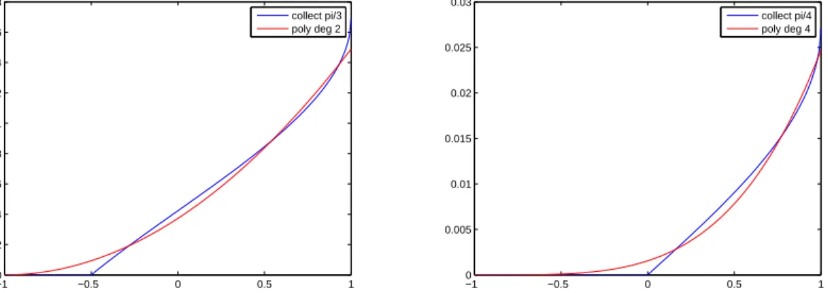
3.1 Kernels corresponding to the collection of all balls inR2 _and _R3 _{. . . .} ₄₃

3.2 Kernels corresponding to cone collections of given solid angle . . . 43

4.1 Example NC classification on the Synthetic dataset . . . 52

4.2 Example NC classification on the Cone-Torus dataset . . . 53

4.3 The synthetic dataset, and an example NCL classification . . . 58

4.4 The dynamics of the individual outputs for various λ. The curves show, for each individual, the average output of a single output node over all points of the corresponding class. The ensemble size is 3. From top left we have a)λ= 0.76, b)λ=λ∗ = 0.75, c)λ= 0.7, and d)λ= 0. . . 59

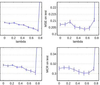
4.5 MSE and MCR on both training and testing sets asλincreases on the synthetic dataset . . . 60

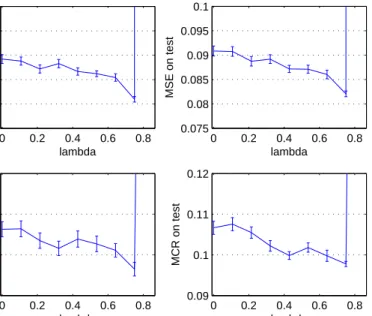
4.6 MSE and MCR on both training and testing sets asλincreases on the cancer dataset . . . 61

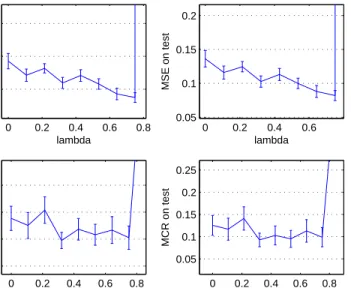
4.7 MSE and MCR on both training and testing sets as λ increases on the liver dataset . . . 62

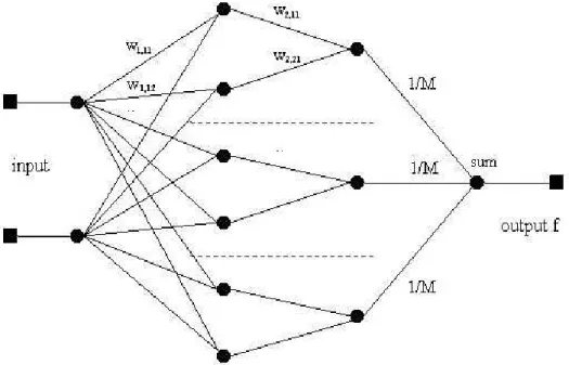
4.8 An illustration of the architecture of an NCL network. The weights shown as 1 N are fixed. For λ= 0 the networks are trained as individuals as indicated by the dotted lines. Forλ=λ∗ the network is trained as a whole. . . 65

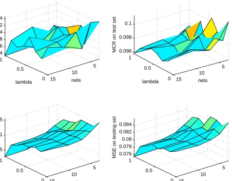
4.9 MCR and MSE for differing numbers of nodes on the liver dataset. The en-semble size is 3. . . 67

4.10 MCR and MSE for differing numbers of networks on the liver dataset. There are 5 nodes per net. . . 67

4.11 MCR and MSE for differing numbers of nodes on the synthetic dataset. The ensemble size is 3. . . 68

4.12 MCR and MSE for differing numbers of nets on the synthetic dataset. There are 5 nodes per net. . . 68

4.13 MCR and MSE for differing numbers of nodes on the cancer dataset. The ensemble size is 3. . . 69

4.14 MCR and MSE for differing numbers of nets on the cancer dataset. There are 20 nodes per net. . . 69

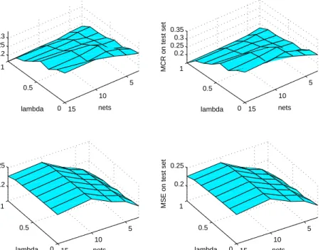
4.15 MCR and MSE for differing numbers of nodes on the cone-torus dataset. The ensemble size is 3. . . 71

4.16 MCR and MSE for differing numbers of networks on the cone-torus dataset. There are 5 nodes per net. . . 71 5.1 An illustration of the individual leaves into which a tree can be decomposed . 75 5.2 A sample of hyperboxes defined by overlaps of leaves in a 20-tree ensemble . 78

(9)

5.3 Performance and complexity of the pruned and unpruned bagging-equivalent

tree for synthetic dataset . . . 80

5.4 Performance and complexity of the pruned and unpruned bagging-equivalent tree for cone-torus dataset . . . 80

5.5 Pruned and unpruned trees built on hyperbox samples for synthetic dataset, against threshold . . . 81

5.6 Pruned and unpruned trees built on hyperbox samples for cone-torus dataset, against threshold . . . 82

5.7 Pruned and unpruned trees built on hyperbox samples for diabetes dataset, against threshold . . . 82

5.8 Pruned and unpruned trees built on hyperbox samples for liver dataset, against threshold . . . 82

5.9 Pruned and unpruned trees built on hyperbox samples for cancer dataset, against threshold . . . 83

5.10 Illustration of the grafting operation . . . 85

5.11 Original ensemble trees . . . 90

5.12 Output merged tree . . . 90

5.13 Tree merging on cancer dataset . . . 93

5.14 Tree merging on cone-torus dataset . . . 93

5.15 Tree merging on liver dataset . . . 93

5.16 Tree merging on synthetic dataset . . . 94

5.17 Tree merging on diabetes dataset . . . 94

5.18 Tree merging on cancer dataset with feature resampling . . . 96

5.19 Tree merging on cancer dataset using error-based pruning . . . 96

5.20 Tree merging on cone-torus dataset using error-based pruning . . . 97

5.21 Tree merging on liver dataset using error-based pruning . . . 97

5.22 Tree merging on synthetic dataset using error-based pruning . . . 97

5.23 Tree merging on diabetes dataset using error-based pruning . . . 98

5.24 Membership function of a hyperbox fuzzy set . . . 99

5.25 Example of a GFMM model on the synthetic dataset . . . 100

5.26 Performance of GFMM models on liver dataset . . . 102

5.27 Performance of GFMM models on diabetes dataset . . . 102

5.28 Performance of GFMM models on cone-torus dataset . . . 103

5.29 Performance of GFMM models on cancer dataset . . . 103

5.30 Performance of GFMM models on synthetic dataset . . . 104

5.31 Complexity of GFMM models on 2-D datasets . . . 105

5.32 Performance of small sample GFMM models on cancer dataset . . . 105

5.33 Performance of small sample GFMM models on liver dataset . . . 106

5.34 Performance of small sample GFMM models on diabetes dataset . . . 106

5.35 Performance of small sample GFMM models on synthetic dataset . . . 107

5.36 Performance of small sample GFMM models on cone-torus dataset . . . 107

6.1 The top line shows the combined performance using training sequences of length 3. Average performance of individual models plotted against percentage of sequences taken as predictions, for training sequences of length 3,4,5, and 6 are the lower plots (from top to bottom line). . . 114

6.2 g value vs Q for individual and combined HMM predictions, using histories as labelled . . . 116

6.3 Performance vs Nearest Neighbor count, for histories and prediction time frame as labeled . . . 118

(10)

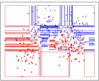
6.4 A plot of a sample of points where the last two events have been complaints. A + denotes churn, a * non-churn. . . 120 6.5 g against lambda for NCL on the churn dataset . . . 121

(11)

List of Tables

4.1 Summary of results for λ = 0 (independently trained networks) and λ= λ∗

(NCL ensemble with de-correlated outputs) . . . 62 4.2 Table of the optimal (in terms of MCR on testing set) parameter settings out

of the experiments performed, for each dataset. . . 70 5.1 UCI datasets used in empirical work . . . 79 5.2 Summary of performance and complexity of approximate bagging trees for a

threshold of 0.8 . . . 83 5.3 Summary of performance and complexity of a merged ensemble of 21 trees . . 98

Notational Conventions

In the table below, common notational conventions and acronyms we will use throughout the thesis can be found. In a few cases, symbols are allowed to have two meanings, and occasional departures from these conventions have been unavoidable. However, in these cases it should be very clear by context what is meant.

(12)

Letter/symbol Meaning

X Input space of features

Y ={ω1, ω2, ...}, Y =R Set of output classesω (or output space in regression)

x Feature vector of an example

y Label of an example

{xi, yi} Set of example/label pairs

K Number of classes

K(x₁,x₂) Kernel function

n Number of examples

m Number of features (dimensionality ofX)

N Number of classifiers, generic cardinality (clear by context)

k Iteration, or model index

L Loss function

h Base learner

M Subset of input spaceM ∈X (model)

M Subset collection

D,D(•) Distribution of examples (of class•) inX

T R Training set

T E Testing set

g,f Functions/mappings

φ Transformed co-ordinates

IM,Icondition Indicator of a setM, or truth of condition

t,τ Node of decision tree, occasionally time

n(t) Number of examples in nodet

e(t) Number of errors in nodet

Tt Subtree rooted at nodet

ǫ Generalisation error

d Target (regression)

E Error function

wi Weight

w·x+b= 0 Hyperplane with normal vectorw

P(•)() Probability (over•). For simpler probabilities, short notation below is used.

p(•) Probability of•

E₍

•) Expectation (over•)

i,j Generic indices used to identify members of a collection

F Power set ofX,F = 2X

µ,µij Class support (of classifierifor classj)

MCS Multiple Classifier System

MLC Model Level Combination

MLP Multiple Layer Perceptron

SD Stochastic Discrimination

NCL Negative Correlation Learning

RF Random Forest

SVM Support Vector Machine

MSE Mean Squared Error

MCR Misclassification Rate

(13)

Chapter 1

Introduction

In many areas of human endeavor, it is necessary to classify things that have been observed, or to identify patterns. Examples of this are everywhere. We communicate using classes; language is in many respects a class system, and is an example of how powerful a good class system can be for extracting and conveying useful information from raw data. An observed object can be classified as a table, chair, spoon, mountain - and we can then communicate a wealth of information about that object to another person familiar with our class system simply by communication of the class. Decisions are also made based on the recognition of patterns, usually with more abstract classes such as ’ill’, ’fraudulent’, etc. The act of classi-fication is the transformation of raw data about an object into concise, useable information in the form of a set of possible, meaningful classes. The human brain is thankfully able to do this very efficiently in many cases.

In order to classify something, we need some sort of model which contains the knowledge needed to identify an unknown object as a particular class. This information is usually learned from a number of examples of objects of that class. Most information about the world can with a little creativity be expressed as a set of numbers (visual data becomes an array of pixels with varying levels of red, green, blue, or greyscale, sizes and many other measurements naturally result in a number, categorical information can be mapped to discrete values of a feature, etc). This realisation, together with the advent of powerful computers and mass storage brings the possibility of expressing classification as a mathematical procedure, a mapping of points in an input space of observations into an output space of classes. In this form it is possible to replicate and automate this human gift of recognising patterns, by creating an algorithm, or sequence of mathematical operations that can be performed using a computer.

The reasons we may want to do this are many. A classification task may need to be repeated many times, or it may need to be done very quickly. It may be too expensive to do it manually, or it may be difficult for humans due for example to the quantity of examples or number of features involved (humans have difficulty visualizing abstract data in more than 3 dimensions). A number of examples of areas of application for classification systems are:

• Fraud detection - credit card, insurance [97], etc; • Customer behaviour prediction [50];

• Speech/image/character recognition [85]; • Quality control - identification of faults/defects; • Process monitoring [132];

(14)

• Medical diagnosis [112]; • Email spam filtering [111]; • Astronomy.

Pattern recognition [32] is a branch of computer science whose aim is to do exactly this; to translate the human ability to identify and classify to a computerised form. It is becoming increasingly more important in commercial settings due to the steady increase in computing power, data storage capacity and the growing usage of computerised systems in all aspects of business, government and research. Huge amounts of potentially useful data are generated and stored daily in all of these areas, however to make good use of it patterns must be identified. The sheer volume of information in many areas makes the use of automated pattern recognition systems highly attractive, if well performing, consistent methods can be developed [96]. As part of this thesis, a classification system developed in the context of telecom churn prediction [50] (predicting when customers may leave a company) will be used as a case study for the potential uses of pattern recognition in industry.

Pattern recognition has in fact two closely related sub-branches, classification and regres-sion [101]. The introduction has focussed on the concept of classification as this is the branch this thesis is most concerned with, but regression should be mentioned also. The difference between the two lies in how the information we try to extract is most naturally represented. In classification problems, we try to extract categorical information - there is no continuum of possible classes, and no concept of ’distance’ between classes. Examples would be clas-sification of images into ’chairs’, ’tables’ and ’bookshelves’, or identification of handwritten letters. In regression, we try to extract continuous information with a well-defined distance measure, for example share price forecasting, or a temperature. We can to some extent recast problems of one form into ones of the other, but it is a little unnatural. For example, given a

K class classification problem, we can cast this as a multiple regression problem by trying to predict each of the continuous probabilities P(classi|data). This is not ideal as the data we have for training is in categorical form, but can still be successful. Similarly, the continuous value to be predicted in regression problems can be discretised, placing values into categories corresponding to some interval. This is even more unnatural as we are essentially throwing away valuable information, but again is useful in some cases. For the remainder of the thesis we will implicitly assume the classification setting, and assume the recasting above whenever we use regression methods for classification.

More mathematically, pattern classification is concerned with labeling an observation with one of a number of identifiers, using knowledge from a number of example observations [11]. An observation is a pair {x, y}, where x is a vector in an input space X = Rm _of

m dimensions, and y exists in Y = {ω1, ω2, ...ωK}, a set of K classes. The elements of x are called features and describe our knowledge of the object. The pattern recognition task is as follows. Given a number n of labeled observations, or pairs {xi, yi}, learn a function

g(x) : X 7→ Y such that, given a new unlabeled example, the new example is labeled with minimal error. This functiong outputs our prediction of the class given an observationx. A mapping such as this is called a classifier. It is possible for an observation with features given by x to be one of a number of classes (our features may not be sufficiently distinctive, so thatg is non-deterministic). For this reason a probabilistic framework is introduced. We let (X, Y) become anRm_{× {}_ω₁_{, ω}₂_{, ...ω}_K_}_{-valued random pair. The probability of a given pair}

(x, y) is governed by the distribution of (X, Y). Then the functiong maps xto a prediction for they∈Y that maximises P(y=ωi|x).

There are many, many ways to represent, train and build these functions, or classifiers. Some of the more popular ones will be covered in Chapter 2. Examples are:

(15)

• Decision trees: Classify examples via a tree-like hierarchy of (usually) binary tests. • Neural Networks: A complex, flexible parametric function implemented through a

net-work of interconnected nodes.

• Kernel methods: The class probability distributions are modeled via a convolution of a kernel with the training data.

This brings us to the important question of how a classifiers performance is quantified, in order to choose which method it is best to use given a concrete problem. The basic challenge when designing a classifier is to minimize the generalization error, the error when classifying previously unseen data. It has been proven, unfortunately, that a universal best classification rule does not exist. For any rule, there will exist distributions on which a different rule will result in a better-performing classifier. This is the rather aptly named No Free Lunch theorem [128]. However, this does not mean that some rules do not perform well on a wider variety of distributions than others.

Given training data {xi, yi}, we have the generalisation error given by ǫ = P(g(x) 6=

y|{x1, ...,xn}), where P is averaged over the distribution of (X, Y). The classifier which would minimise this probability of error is called the Bayes classifier; the minimum however is only zero for distributions such thatP(y|x) = 1 for some y, and for allx whereP(x)6= 0. In general the Bayes error is non-zero and an error free classifier is not possible, however we can still strive to build a classifier which performs well in most situations. The performance of a classifier is usually predicted using a separate testing dataset, unseen during training, or using cross-validation.

There are numerous challenges when attempting to build a well performing classifier [52]. Some of these are as follows.

• Poor/insufficient data. The methods used to label the data used in training are usually expensive, difficult and/or time consuming. If this was not the case there would be little motivation to automate. Therefore one challenge in pattern recognition is to build a well performing classifier using minimal data. Data may also be noisy, include features that are mostly irrelevant for the classification problem, or be incomplete. This poses the additional problem of maintaining reasonable performance over a range of data quality.

• Adaptability. In some application areas the input space, or the relationship between output and input, changes over time. A good example of this is spam filtering. The pattern here is the sequence of letters/words in an email, with a binary classification scheme into spam and non-spam. As filters (classifiers) improve, the perpetrators of spam attempt to fool the filter by miss-spelling words and numerous other strategies which attempt to shift the location of their spam in the input space into an area which would be classified as non-spam. Spam filter software must be able to continually adapt to these shifts and maintain good performance.

• Generalisation. In order for a pattern recognition scheme to be useful, we must know the performance we can expect from it. Thus some way of predicting a classifiers performance is necessary. Good performance of the classifier on the training data is not enough; it must generalise to new unseen observations. This is closely related to the complexity of the classifier, and will be discussed in greater detail later. In brief, an overly complex function can tune itself very closely to its training data. When this happens a classifier may fit itself to outliers and noise in the data, and may perform very

(16)

badly on new points in a phenomenon called over-fitting. It is also related to the length scale over which the function changes - if the fitted function has detail on a length scale smaller than the distance between training points, it is likely we will overfit.

• Curse of dimensionality. As the dimensionality of the data increases, a sample of a given size becomes sparser and most of the input space becomes empty. This can result in poor performance of many classifiers, and also makes it hard to visualise the data and resulting model.

Historically a variety of methods have been proposed to overcome these challenges. Pre-processing of data can help improve the quality of data by for example attempting to remove outliers. There are also methods to reduce the dimensionality of the data while retaining essential information, mitigating problems related to irrelevant features and the curse of dimensionality. Regularisation [6], pruning, cross-validation [20] and other methods were developed to control complexity or predict performance in some classification schemes, and so reduce over-fitting.

Different classifiers may have a similar performance while giving significantly different decision boundaries. This suggests they extract slightly different information from the data; the fact that there is no single best classifier for all problems also supports this view. Given this insight, the idea of combining classifiers was proposed to help solve some of the above problems. It has parallels with the way humans sometimes make decisions - important de-cisions are often not made by one person alone, but are the combination of the dede-cisions of many people, for example in a vote. The combination of classifiers will be the focus of this thesis.

Classifier combination first began to appear a few decades ago and rapidly gained pop-ularity. It is now a vibrant area of research with a huge literature, both algorithmic and theoretical. Its main attraction is improving the consistency of predictions by reducing vari-ance [70], thus improving the performvari-ance. Some methods may also reduce bias; the concepts of bias and variance are explained further in Chapter 2. A combined method reaches deci-sions using a number of different base classifiers, or representations of the data, or parameter settings, and as such is intuitively less subject to the vagaries of the individual. Where some individuals would perform poorly in a specific problem or sampling of data, the combined classifier should still retain reasonable performance. In addition to a method of building a single classifier from data, there are two further elements necessary in the classification framework to build a combined classifier, or Multiple Classifier System (MCS). Intuitively classifiers must be diverse in order for gains to be made via combining, meaning some method of diversifying classifiers is the first of these. The second element is the rule defining how a final classifier is built from the individuals.

There are many ways of diversifying classifiers [18], and Chapter 2 will cover those found in the literature. In overview, classifiers can be diversified mainly by changing the data used to build them in various ways, or by changing the algorithm (rule) used to build each classifier. Naturally in most combination schemes the individual performances are also important. It is an ongoing challenge to find the most useful form of diversity for combining, and to find methods of generating many classifiers that are both well-performing and diverse.

We also have numerous options for the final vital piece in a combination approach, the combination method itself [75]. There are many ways of combining the outputs of many classifiers, or we may opt to combine individuals at the model level. Again these methods can be found in the literature review in Chapter 2. There are a few basic paradigms that can be followed when building a MCS, both in the creation of the ensemble and in the method of combination. In building an ensemble, we may create individuals from which we will select a

(17)

subset to build the final classifier, or individuals all of which will be used in the final classifier. Which paradigm we follow guides our choice of diversification method, as we must be more careful and principled in the individuals we create when all are expected to take part in the final classifier. We will focus more on this latter, as we feel that this paradigm fits better with the structured, theory-driven approach we wish to take to classifier combination.

In combining, there are three conceptually different approaches. The first, and probably the simplest, is decision level combination. For a point x, some function of the decisions of each classifier in the ensemble on that point is used as the final decision. Letg1(x), ..., gN(x) be an ensemble of N classifiers. The outputs of each classifier on the point define a vector in the N-dimensional intermediate space G of the ensemble. The final decision is given by a function f mapping points in this intermediate space to the set of classes Y, that is

f : G → Y, f = f(g1(x), ..., gN(x)). This function is usually relatively simple; an oft-used example is majority vote, where the function f is simply the mode of the g’s.

A second approach is to allow different classifiers in the ensemble to make the decision on a point, depending on where in the input space this point lies. This is based on some measure of the competence of individual classifiers in an area of the input space. Given a new point x, the competence of each classifier at x is calculated and the point is classified using the classifier with highest competence. This results in a partition of the input space. This could alternatively be cast within the first paradigm by allowing the function f to depend onx.

The third is to combine components of the structure of individual classifier models to make a combined classifier of similar type. Again these concepts will be covered in more detail in the literature review.

There are very many proposed frameworks for building combined classifier systems, and many are based mostly on heuristics and ad hoc ideas. One of the challenges of the field is solidifying the basis on which combined methods are built. What is needed [65] is a concrete theoretical framework identifying the properties of an ensemble which control performance, and quantifying the dependence of the performance on these parameters. Understanding of how well these parameters will generalize if we enforce them on a training set is essential for relating any theory to generalization errors. This involves relating measures of diversity and individual performance to combined performance, and developing methods to consistently build classifiers with the desired properties. Decompositions of the error, such as generalised bias variance decompositions and ambiguity decompositions (see Chapter 2), can help and some methods which build upon this basis will be covered later (in particular in Chapter 4). The framework of Stochastic discrimination which we will introduce in Chapter 3 also goes some way toward providing a solid theory.

The aim of this thesis is to contribute to the development of combined classification methods, in both algorithmic and theoretical directions. Its structure will be as follows. We start the main body of the thesis with Chapter 2, a literature review of topics relevant to MCS, and elaboration of some of the topics mentioned in this introduction. The aim is to build a solid understanding of the issues that arise when building a MCS and methods in the literature developed to address them.

The Stochastic Discrimination (SD) framework [67] is introduced in Chapter 3 as a theo-retical structure in which we can understand the properties of a collection of subsets necessary for successful combination. We will see how properties defined within this framework are en-couraged by some of the more popular methods in the literature, and forge some interesting links between the methods.

A method called Negative Correlation Learning (NCL) [84] is introduced in detail in Chapter 4. It is a neural network combination method where networks are trained in parallel with error functions designed to encourage useful diversity. The form of the error function

(18)

for each network is based on the ambiguity decomposition (see Section 2.1), and has a term that penalises similarity to the other networks in the ensemble. The importance of this term is governed by a parameter lambda. A theoretical investigation into the effects of lambda on the dynamics of the training is the main subject of this Chapter, with some empirical observations from other papers explained and an optimal (in some sense) lambda derived. This is backed up by experiments.

Chapter 5 looks in more detail at the Model Level Combination (MLC) paradigm men-tioned previously. This paradigm has seen by far the least coverage in the literature, and this section will introduce a few new methods in MLC. Two methods of building a decision tree whose structure is built by combining components of an ensemble of different trees are intro-duced. In addition, a similar method which uses an ensemble of trees to provide a base set of hyperbox fuzzy rules to be combined using a modified GFMM (General Fuzzy Min-Max) framework [47] is presented.

An application of pattern recognition, and MCS in industry will be the subject of Chapter 6, with churn prediction in the telecommunication domain used as a case study. A churn event occurs when a customer ceases to use some service a company offers, and naturally companies wish to avoid this if possible. Churn prediction is the prediction of these churn events from customer history information. Prior warning that this may occur allows companies to take action to retain the customer, for example by offering a small incentive to stay. The methods covered in previous chapters will be applied to this problem, together with other methods from the literature which are particularly well suited for this problem. Some issues of data relevance horizon (length of history to be used in prediction) are investigated, to guide our choice of data to use when trying to predict churn.

Conclusions, comments on future work and a brief summary of the thesis will be presented in the final Chapter, Chapter 7, and followed by References and Appendices.

The original contributions of this thesis can be summarised as follows:

• A synthesis of existing and original links between some popular methods in the lit-erature, within the framework of Stochastic Discrimination (SD). These methods are Random Forests, Stochastic discrimination (a classification method developed in par-allel with the framework by its author), Support Vector Machines, and Boosting. The methods are cast as inducing a kernel on the training data with desirable properties, with classification performed by a separating hyperplane in the transformed space cor-responding to this kernel. The use of the SD framework to understand these methods, and the links between SD and the other three methods in particular constitutes an original contribution.

• A theoretical analysis of various aspects of the Negative Correlation Learning method, in particular regarding the effects of an important parameter,λ, on the training stability, performance and complexity of the model built. This culminates in a derivation of a value λ∗_{, depending only on} _N_{, for which properties of the training are particularly}

desirable, and a range of λ over which training is stable. This theoretical work is illustrated and tested empirically on a number of datasets.

• A proposal and investigation of three new methods for the model level combination of multiple decision trees. These are:

– Building and pruning the bagging-equivalent single tree. This is done both directly (on low dimensional datasets), and more generally in an approximate fashion. The approximation is built by sampling leaves of the full bagging tree using a Monte-Carlo method, and building a tree on these sampled, labelled hyperboxes. We also

(19)

experiment with pre-pruning of the samples before tree-building, both combined and contrasted with standard post-pruning.

– A tree merging method in which we generalise bottom-up tree pruning to a tree ensemble context, simultaneously combining and pruning the trees in the ensemble in parallel. This is done by allowing grafting of subtrees from one ensemble member onto a node of another. A modification of single tree pruning criteria is proposed for use in this context, and tested empirically.

– A method combining hyperboxes sampled (in the same way as above for the bagging-equivalent tree) from overlaps of trees in a bagging ensemble within the GFMM framework. Pre-pruning of samples before combination is also investigated here.

These methods provide a useful alternative when performance is not the sole require-ment, as while the methods cannot compete performance-wise with the best decision level methods, extremely compact and understandable models are produced. As a by-product of the above investigations, an interesting theoretical link between minimum error pruning and pessimistic pruning is derived.

• A combination method developed for application to the telecommunications churn pre-diction problem. Additionally, the investigation of the relevance horizon of customer data on this problem led to the development of a non-sequential representation of the sequential raw data, allowing additional classes of predictor to be used on the problem with some success.

The list of publications that have resulted from this thesis are as follows: • The Dynamics of Negative Correlation Learning [35]

• Lambda as a Complexity Control in negative Correlation Learning [1]

• A Non-sequential Representation of Sequential Data for Churn Prediction [37] • Building Combined Classifiers [36]

(20)

Chapter 2

Literature Review

In this Chapter we review the ensemble methods literature and a few related areas which will be necessary for the understanding of later chapters. Literature related to the churn prediction application investigated in Chapter 6 will be delegated to that Chapter, as it would be of little help before the application area itself is introduced, and is not necessary for understanding of previous chapters.

2.1

Error Decompositions

The most important measure of the performance of a classifier is the generalization error [11]. It is the reduction of this that provides the driving force behind the development of multiple classifier systems. Therefore we will start by looking more closely at the ensemble error and how it depends on properties of the ensemble. Intuitively, we would expect that the error of an ensemble of classifiers would depend on the individual errors of the classifiers, and on some parameter(s) encoding the interaction between the errors of the classifiers. The form of the dependence would be expected to vary between combination methods. The decompositions below can help explain why certain combination methods work, in a similar way to the framework we will introduce in chapter 3.

2.1.1 Squared Loss

The following decompositions attempt to quantify this intuition, for the ‘easy’ case of regres-sion problems. In this case squared loss and (weighted) averaging are the natural choices for loss function and combiner.

Bias-Variance Decomposition

Starting with a single predictor, we have the bias-variance decomposition [48]. Assume our training data T R = {xi, di} is sampled from an underlying distribution D. We want the average error of our predictor, not an error for one particular sampling, so we consider the expectation E_{T R(}_ǫ_{) over all possible training sets} _{T R} _{sampled from} _D_.

E_{T R(}_ǫ_{) =} E_{T R(}_f₋_d₎2 _(2.1)

= E_{T R}(f+E_{T R}(f)−E_{T R}(f)−d)2 (2.2) = E_{T R}_[(_f ₋E_{T R}₍_f₎₎2_{+ (}E_{T R}₍_f₎₋_d₎2_{+ 2(}_f ₋E_{T R}₍_f₎₎₍E_{T R}₍_f₎₋_d_{)] (2.3)}

(21)

The first term is the bias, indicating the loss when using the expected value of f to predict

d. The second term is variance, and gives us the expected added loss of using one particular

f whose average squared deviation fromE_{T R}₍_f_{) is the variance. When we have an ensemble}

of N predictors, f becomes PN

i=1wifi, a weighted average of the outputs of the predictors. For an unweighted averagewi = _N1 the expression reduces to:

E " 1 N X i fi ! −d #2 =bias2+ 1 Nvar+ 1− 1 N covar (2.5) with bias= 1 N X i (E₍_f_i₎₋_d₎ _(2.6) var= 1 N X i E(fi−E(fi))2 (2.7) covar= 1 N(N−1) X i X j6=i E{(fi−E(fi))(fj −E(fj))} (2.8) so we have a decomposition which is dependent on the components of the individual errors, and an interaction term (the covariance). The first term is the ensemble bias, the other two terms together are the ensemble variance. If the predictions of all the ensemble members are independent the interaction term is zero. In this case the variance component of the ensemble error is reduced by a factor of _N1 compared to the average variance of the individuals. For dependent (correlated) predictors the variance is reduced by a different factor which has been shown [121] (assuming a common varianceV for all classifiers) to be:

V_ensave =V 1 +δ(N −1) N (2.9) where δ is the average correlation between predictions over all pairs of predictors. The im-plication of this is that if we have predictors whose error is dominated by variance, then by combining we can potentially gain large improvements over any one individual. Larger improvements are gained for smaller δ (lower correlations) and higher N. The difficulty of course is the generation of uncorrelated predictors. We can attempt to generate N uncor-related predictors while maintaining individual accuracy, but this gets more difficult as N

increases. Some methods of doing this will be covered in later sections. Chapter 4 will analyse one of these methods in greater detail

Unfortunately, in classification tasks decomposing the error is not so easy. Here the final output of a classifier is one of a few discrete class labels. It is either the right label, or not; there is no concept of ‘distance’. The labels could be numbers, but could just as easily be strings or anything else, so it is not clear how to define bias and variance. Certainly the standard definitions are of no use as they assume the space of possible output is closed under addition/multiplication/division. This is not true for the classification case even if we use numeric labels (which we can always do). In cases where the output label is based on some continuously varying value with a specific target value, such as classifiers which approximate the posterior probabilities of the classes, progress can be made. As Tumer and Ghosh have shown [120], the squared error of the posterior estimates can be linearly related to the squared error of the classifier decision boundary in approximating the true boundary. This is done by assuming that the posterior probabilities are monotonic in the boundary region, and that the approximated boundary is close to the true boundary. Under these assumptions, the

(22)

estimated posteriors at the point where they are equal (on the estimated boundary) can be linearly expanded around the true boundary. This results in:

b= ǫi(zb)−ǫj(zb)

p′_j(z∗₎₋_p′

i(z∗)

(2.10) where ǫi(zb) is the error of the classifier in approximating the posterior probability of class

ωi atzb, andbis the distance between the estimated boundaryzb, and the true boundaryz∗. The denominator is a constant over different training sets and so does not need to be known. In turnb2 can be shown to be directly proportional to the classification error rate. Thus the bias-variance decomposition described above can be used in this case, as we have related the misclassification rate to a squared error, even if only approximately. Many classifiers (such as the tree classifier) cannot approximate the posterior probabilities in this way. Definitions of bias and variance suitable for use with general loss functions when the classification problem cannot be linked to a regression problem are given in Section 2.1.2.

The Ambiguity Decomposition

Another extremely important result due to Krogh and Vedelsby [72] for combining predictors in the regression context is the ambiguity decomposition:

(fens−d)2 = X i wi(fi−d)2− X i wi(fi−fens)2 (2.11) This gives us a direct decomposition of the ensemble error into the average of the individ-ual errors and a second term containing all interactions, called the ambiguity. It is reached via similar manipulations to the bias-variance decomposition. Because the second term is positive definite, in the case of regression problems we are guaranteed an improvement over the average of the individual errors when combining. It also shows us that, keeping the aver-age error of the predictors in the ensemble constant, we can reduce the ensemble error simply by increasing the second term, making our predictors spread as widely about the ensemble mean as possible. We will see some ensemble methods among those described in Section 2.4 for which this decomposition provides the driving force, and will look at one in particular in more detail in Chapter 4.

2.1.2 General Loss Functions

In this section we will describe some of the bias-variance decompositions which have been proposed for more general loss functions, one example of which is the zero-one loss widely used in classification. The fact that a single decomposition cannot be given in this section illustrates the current state of uncertainty in this area. It is an open question which of the current definitions is more useful, or whether it is possible to do better than the current definitions. The following two definitions have been derived specifically to provide an additive decomposition of the error as well as encoding characteristics of the distribution of outputs of different classifiers, and so are obtained starting from the expected error at a particular point x:

P(error|x) = 1−X i

PD(ωi|x)P(ωi|x) (2.12) where P(ωi|x) is the probability a given point x has true class ωi, and PD(ωi|x) is the expected probability over all possible training sets sampled fromD that it would be labeled

(23)

ωi. Adding and subtracting extra terms whose sum is 0, and grouping the terms can result in different potential expressions for bias, variance and noise (Bayes error).

There are certain desirable characteristics we would like definitions of bias, variance and noise to have. These are:

1. Any generalized definitions must reduce to the standard definitions in the case of squared loss.

2. The variance should be non-negative, and should be 0 for a classifier which disregards the training data.

3. The bias should be zero for the Bayes optimal classifier.

4. The definitions should provide an additive decomposition of the error.

As we shall see below, finding definitions which satisfy all these constraints is difficult. Kohavi-Wolpert Definitions

Kohavi and Wolpert [69] propose the following definitions:

bias = 1 2 X ωi (P(ωi|x)−PD(ωi|x))2 variance = 1 2 1− X ωi PD(ωi|x)2 ! noise = 1 2 1− X ωi P(ωi|x)2 !

The interpretation of the terms is as follows. The bias is the sum over ωi of the MSE in approximating the posteriorsP(ωi|x) with the probability over all training sets of a classifier predictingωi. The variance measures the spread of labels assigned to xby classifiers trained on different training sets, and is related to the Gini index sometimes used in decision trees. Using this definition of variance, the noise is then the variance of the Bayes classifier. The Kohavi-Wolpert definitions above suffer from a bias term which may not be zero for the Bayes optimal classifier, violating requirement 3. One advantage however is that it is a continuous functional of the underlying distribution; An infinitesimal change in the underlying distribution will result in an infinitesimal change in the above quantities. For the next set of definitions given by Breiman this is not the case, as we will see.

Breiman’s Definitions

Breiman’s definitions [14] provide an alternative decomposition for which the bias of the Bayes classifier is zero.

bias = (P(ω∗|x)−P(ωˆ∗|x))PD(ωˆ∗|x)

variance(‘spread‘) = X ωi6=ωˆ∗

(P(ω∗|x)−P(ωi|x))PD(ωi|x)

(24)

Hereω∗ is the label with the highest true probability givenx, i.e. it is the decision of the Bayes classifier. The label which is the most probable output for x over classifiers trained on random samples fromDis ωˆ∗_{. Thus the noise is the error of the Bayes classifier, the bias}

is the expected additional error of using ωˆ∗ to label x instead of ω∗, and the variance is a measure of the spread of outputs over classes other thanω∗ andωˆ∗.

Each set of definitions have their own advantages and disadvantages. Breiman’s bias satisfies requirement 3, but the variance does not satisfy 2. It may be negative, and a classifier which ignores the data may not have zero variance, and in fact may not even minimize the variance. The bias and variance may also be discontinuous given an infinitesimal change in the underlying distribution. If this change causesωˆ∗ to change, then althoughPD(ωˆ∗|x) will change only infinitesimally,P(ωˆ∗|x) will not in general.

James’ and Domingos’ Definitions

James [59] has taken a slight departure from the approach taken in the previous two decom-positions. The above definitions attempt to characterize in a sensible way the output of a classifier by some measure of its systematic deviation from the target value over all possible training sets and by its variation about its systematic value for differing training sets. At the same time they also try to provide an additive decomposition of the error. James argues that for general loss functions we cannot define a quantity which does both jobs well, and proposes to split this dual role into separate definitions. By doing this he is able to satisfy all the properties an intuitively sensible decomposition into bias and variance should have, but at the cost of having a dual definition. He definesL(y, d) to be the loss, or cost incurred ify is predicted when the target value is d. The prediction y is the prediction of a classifier built on a particular training set sampled from the distribution of training examples D. In the following, expectations are over training/test sets sampled fromD. He proposes:

Define

y∗=argminγ(E[L(y, γ)]) (2.13)

to be the systematic part ofy (and similarly for d). Then Bias, Variance and Noise are:

B = L(d∗, y∗) (2.14)

V = E_[_L₍_{y, y}∗_)] _(2.15)

N = E_[_L₍_{d, d}∗_)] _(2.16)

and further define

V E(y, d) =E_[_L₍_{d, y}₎₋_L₍_{d, y}∗_)] _(2.17)

SE(y, d) =E[L(d, y∗)−L(d, d∗)] (2.18) WhereV E(variance effect) andSE(systematic effect) give the effects of bias and variance on the error, providing an additive decomposition. He shows experimentally that there is usually a high correlation between bias and SE, and variance and V E. For the special case of squared error loss, the definitions for variance andV E coincide and become the standard definitions, as do the bias andSE.

Domingos [30] uses the same definitions of bias and variance, but show that for certain loss functions, the error at a point xcan be decomposed as follows:

(25)

Specifically, for zero-one loss the coefficients are:

α1 =PD(y =d∗)−PD(y=6 d∗)PD(y=d|d∗ 6=d) (2.20)

α2 = 1 if y∗=d∗, and α2 =−PD(y=d∗|y6=y∗) otherwise. (2.21) An interesting property of this is that for points on which the classifier is unbiased (y∗₌ d∗) the variance adds to the error, and for biased points it subtracts from it. This does not violate requirement 2, as the variance itself is always positive. This is intuitive - if the classifier consistently predicts the wrong class for a point, then the more often it varies from this most probable prediction, the more likely it will ‘accidentally’ give the correct class.

Domingos also points out that for two class problems the margin (see below) can be written in terms of the bias and variance as defined above:

M(x) =±[2B(x)−1][2V(x)−1] (2.22) with a positive sign ify∗=d∗, and negative otherwise.

Bias-Variance Decomposition and Combining SVM

Now that we have presented these alternative bias-variance decompositions, it would be illus-trative to give an example of their use from the literature. In [124], Domingos’ decomposition is applied to ensembles of support vector machines, to look at how the bias/variance of the models changes when using different parameters for the model.

The interesting points to come out of this analysis are as follows. The authors find that the SVM has quite a large ’stability’ range where good performance is achieved and sensitivity to parameters is small. Bias is low, with the error concentrated mostly in un-biased variance. Parameter choice within this range does affect the distribution of the error between terms, but has little effect on their sum. This can be used to guide ensemble building. Firstly, it can be inferred that bagging, as a method which does well given low-bias high variance base learners, should be a good choice for SVM ensembles. Secondly, by varying parameters over the stable region we can obtain classifiers with similar overall error but whose error is distributed differently over the terms of the error decomposition. We can then use the distribution to choose classifiers that are diverse in some sense and this may help when constructing an ensemble.

Ambiguity Decomposition for General Loss

There is currently no direct analogue to the ambiguity decomposition for general loss, and some debate as to whether one is possible at all. This is a very important question that needs answering. The ambiguity decomposition relies on the fact that the function g(α) =

P

iwi(fi−α)2is a convex, symmetric (about ¯f) function ofαfor givenfi, with minimum at ¯f so that the distance|d−f¯|is unique for a giveng(d)−g( ¯f) =P

iwi(fi−d)2−

P

iwi(fi−f¯)2. It is hard to imagine an analogue of this concept for something like zero-one loss.

For classification the ‘ambiguity’ type term which measures the effect on error of the correlations between classifiers is not known, and so a variety of measures of ‘diversity’ or the effect of correlations can be used instead (reviews are given in [18], [127], [79]). Many of these are pairwise measures which measure 1st order coincidences of correct and/or incorrect classification. These ignore higher order coincidences and thus are not particularly well-correlated with the ensemble error. A more general framework of arbitrary order coincidences has also been developed [107], and other non-pairwise measures such as entropy. These may have a higher correlation with error, but lose their simplicity of interpretation and so are of

(26)

less use for guiding ensemble creation. The extreme case of this is to use the (normalized) ensemble error directly [105], as we can always measure the ambiguity-like term simply by calculating the difference between the average errors and the ensemble error. This can be very useful for searching for the best subset of classifiers from a pool, but it gives us no information about the characteristics of the subset resulting in a high/low value. Thus it is of no use for guiding how we generate classifiers beyond telling us how good a subset is once it has been generated.

There are theoretical analyses available for certain combination methods which provide some sort of guideline for the patterns of errors of individual classifiers which result in larger improvements in the error of the ensemble. These results provide guidance in the same way as the ambiguity decomposition, but in a much more vague and less useful way. We will briefly describe some of these.

The patterns of success and failure [74] for majority vote ensembles, tell us how it is best to distribute the errors if we have classifiers of given error rates, and we can distribute these errors over examples as we wish. Minimum ensemble error is when we either have examples voted correctly by only one vote, or examples voted unanimously incorrectly. The worst case is if examples are voted either unanimously correct, or incorrect by only one vote. These error distributions are however unstable as they correspond to the minimum margin (see below). Modified, stable patterns of success and failure have been given in [106].

There are some theoretic results [44], [102] giving the pattern of classifier accuracies where weighted averaging (WA) is more effective than simple averaging or single best. Generally two factors decide this. First, the larger the difference between the errors of the best and worse classifiers, the more improvement will be seen for WA. Second, the more the ‘good’ classifiers are in the minority, the better WA performs.

The theory of margins [113] attempts to explain the success of boosting and support vector machines [25] by the way that the certainty of the decisions are maximized. The margin is the difference between the support given to the correct class, and the maximum support for any other class. Small changes in the training data will cause very little change in the classifier decisions with large margins. This will result in a more stable and hopefully more accurate classifier.

Finding a framework within which the classification performance of ensemble methods can be understood is an open problem. The Stochastic Discrimination framework we will look at in Chapter 3 is a powerful candidate for such a framework. Properties are defined specifying how a collection of subsets should be spread over training points in order for combination of those subsets to be successful; a number of ensemble methods can be understood within this framework. We will illustrate this in detail in Chapter 3.

(27)

2.2

Random Generation of an Ensemble

In Section 2.2 we have looked at some decompositions of the error and found that for regres-sion problems, to make the most of an ensemble of classifiers the ambiguity decomposition defines two quantities of interest. We can of course try to improve the individual performances and so lower the first term in the ambiguity decomposition. Given an average individual error we can also reduce ensemble error by trying to maximize the ambiguity term, making the in-dividual predictions as different as possible. For classification problems it is not so clear-cut, but we know that a similar principle applies and we can generally get better performance by having individuals which make different errors even if we do not know an exact relationship. In subsequent Chapters we will need to create classifiers which differ in some way; this section and the following one will describe some methods for acheiving this. Whether all the classi-fiers generated are expected to take part in the final classifier or whether a search/selection stage will be implemented to decide a subset of the ensemble to combine is an important consideration when generating classifier ensembles. Different generation methods naturally lend themselves to one or the other of these. The methods described in this section create differences randomly, and can be useful in both approaches above. Others described in Sec-tion 2.4 are more directed in the characteristics of the differences they introduce, and are generally more suited to the first approach.

It is first worth mentioning, that while we may try to generate classifiers with independent errors, and theoretical work often assumes this to be the case, in reality the classifiers in an ensemble are nearly always correlated to some extent. Some papers explore the effect of these correlations, either theoretically (under strong assumptions) [121] or empirically [34].

A simple way to make classifiers different is to change something (anything!) randomly and hope that we will get different classifiers out at the end. The methods in this section follow this philosophy. There are a variety of things we could potentially change.

2.2.1 Changing the data

If we change the data somehow before training each classifier, we can expect each classifier to differ in some way. We must compromise between changing the data more to make classifiers differ more, and changing it less so that classifiers will still perform well on the ‘real’ data. Possibilities are:

• Adding random noise;

• Using random subsets or feature subsets; • Applying random transformations.

The idea behind these methods is to gain a number of different samplings or represen-tations of the underlying distribution based on the original distribution. By training com-ponents of the combined classifier on these different representations, it is expected that the combined classifier will be less training-set specific. Therefore the classifier could be expected to generalize better and be more stable.

Adding Random Noise

To generate a new classifier using this method, a training set is created by adding a random vector to each input vector of the original data. The added noise is usually isotropic and gaussian. The width of the gaussian may change for each point or may be the same for all

(28)

points of a given class. The most intuitive way of varying the widths would be to relate it to the density of points in a neighborhood, so that points in less dense regions are spread more. Any number of noisy points may be generated from each training point to give larger noisy sets, or each new point can be generated by randomly picking a training point and adding noise to it. This would be equivalent to combining the ideas of bagging (see next subsection) and random noise. There is a compromise between adding noise with a wider distribution in order to further de-correlate the classifiers, and adding less noise to maintain individual accuracies. As was seen in Section 2.1 both de-correlation and good generalization performance of the individuals contribute to good ensemble performance.

The adding of noise has been explored to a limited extent in [49] however there is relatively little in the literature exploring this in the context of multiple classifier systems. This is perhaps surprising as the aim of a classifier is to try to ‘fill in the gaps’ in generalizing to non-training-set points. Exploring methods of splitting this filling of gaps between the data level and the algorithmic level would seem a sensible approach. Usually only the extreme cases are used. The parzen window classifier can be thought of as one extreme of such an approach. If one imagines generating a dataset of size r|T R| by randomly adding noise to the points inT R according to some kernel, and applying a multinomial (histogram) classifier of N bins to the resulting dataset, then in the limit of {r → ∞, N → ∞ :r/N → ∞} the resulting classifier would tend to a parzen classifier with the same kernel as that used to generate the noise. The other extreme is the more usual case where spaces are filled entirely on the algorithmic level, for example a tree classifier. It would be interesting to investigate intermediate cases, especially in the context of multiple classifier systems as each data level filling of points would be different.

Re-sampling Techniques

The idea behind resampling techniques is to simulate different samplings from the underlying distribution by instead sampling the original training data. The samples can be of any size, with or without replacement. In the most usual implementation, called bagging [12], the samples are the same size as the original training set and are sampled with replacement. Such samples are called bootstrap replicates of the original dataset. More generally, when choosing a size for the subsets there is again a tradeoff between smaller subsets enabling larger numbers of relatively uncorrelated datasets, and larger subsets which are more likely to be representative of the underlying distribution. Bagging has been explored by various authors and is known to be an effective way of generating ensembles. It’s effectiveness can be explained by the reduction of variance [21]. Further, subject to some fairly strict assumptions as to how the error is related to the displacement of the error from the true boundary (as in Section 2.1 and [119]), the bagging error can be derived [45] as:

ǫ=ǫb+ET R E2 T B|T Rǫ(xb(T B);T B) + 1 N[VT B|T Rǫ(xb(T B);T B)] (2.23) This shows that the added error (over the bayes error ǫb) of the N bagged classifiers due to displacement of the predicted boundaryxb from the true one is given by the expected error of a bagged classifier over all bagged training setsT B from training setsT R (which is simply the bias error of a bagged classifier), plus a second term which is _N1 times the expectation over T R of the variance of the bagged classifiers.

The consequences of this are:

• Bagging can be expected to work well with base classifiers which are unstable, and hence have high variance.

(29)

• As the bagged ensemble becomes large, its error approaches the bias of an individual trained on a bootstrap of the original training. data.

• Larger ensembles should perform strictly better, though with diminishing returns for large N.

• The bagged ensemble should perform strictly better than an individual trained on a bootstrap of the training data - note this does not imply better performance than an individual trained on the training data, though one can imagine this will mostly be the case given individuals with a large variance, as is confirmed by empirical results. A method related to bagging is the random subspace method [53] in which a different random subset of features is used for each classifier. Obviously this is only useful for fairly high dimensional data for which there are many potential subsets of features which could be used. For these problems it can be very effective because the ratio of the dimensionality of the problem presented to each classifier to the number of training examples presented is lowered, potentially making the problem easier to handle and quicker to solve. Because of this and the fact that each classifier is trained on all training points, this method tends to work better than bagging for small training sets [116].

The methods above are specific examples of a more general class of method which have been very successful. This class of method was first identified by Breiman in [16] and given the name Random Forests. The formal definition of a random forest ensemble is a set of N

classifiers each grown according to a random vector of parameters Θk. Each element of the vector controls some aspect of the growth of a tree classifier. In practice what is often done is to create a bootstrap sample for each tree to be grown on. During growth of the (unpruned) tree, for each node a random feature is selected for splitting. In this case the random vector would have a set of n random elements defining the index of each training sample in the bootstrap replicate, and another set of random elements giving the feature for splitting at each node.

This method has similarities with a number of other methods; we will look at these links in more detail in Chapter 3.

Applying random transformations

The idea behind this method is to create different classifiers by first transforming the data in some way so that although the same data is used each time it is presented to the classification algorithm in a different way. One way of doing this which has been explored by Sharkey [114] is to pass the inputs through different untrained or incomplete neural networks to create the training sets for each ensemble member. New examples to be classified are first passed through the distorting nets.

2.2.2 Changes in classifier generation

A classifier is a rule generated from the information in the training data, which predicts the class of an input object. If we do not change the data, then in order to get different classifiers we must change how the rule (classifier) is generated from the data instead. Possibilities are:

• Using different base classifiers;

• Changing parameters within a particular base classifier; • Stochastic discrimination.

(30)

Differences in Base Classifiers

One way of getting classifiers with different decision regions from the same data is to use different algorithms to generate them from the data. If an algorithm has some variable parameter which controls some aspect of how it generates a classifier from the data, the same effect can be gained by varying the parameter for each classifier while using the same algorithm. Examples of this approach include the following:

• The random forests method already covered could just as easily have been placed here due to the way in which the growth of the tree is changed between members of the ensemble.

• Combinations of different base classifiers using various searching algorithms and selec-tion criteria have been explored in [108].

• Methods of building ensembles of neural networks with different architectures have been proposed, and will be covered in later Chapters (see Sections 2.4.2 and 2.5.7).

(31)

2.3

Deterministic Generation of an Ensemble

Many of the methods in the previous section also have deterministic counterparts, where sim-ilar things are changed but in a more deterministic way to achieve well defined relationships between individuals. The advantage of these methods is that they do not rely on chance to provide us with complementary classifiers but will instead directly generate them. Often this means we have to generate fewer classifiers than in random methods. These methods tend to lend themselves more naturally to direct generation of ensembles as opposed to generating a pool to be selected from. The downside of these methods is that they require from us a greater understanding of the properties of an ensemble which enable us to build a good combined classifier. If we are not going to rely on chance, then we need a clear idea of how we want the classifiers to differ. This is where the ideas of Section 2.1 can be very useful, though unfortunately the ideas there in the case of zero-one loss are not yet well enough developed to provide exact guidance. Because of this many ideas are still ad hoc to varying degrees, without a well defined theoretical underpinning.

2.3.1 Changing the Data

Among the deterministic methods of changing the data are:

• Re-sampling/re-weighting the data according to some criterion. The major example of this method is boosting, in which the criterion is related to the difficulty in correctly classifying a point.

• Training classifiers on different feature subsets chosen/generated via some criterion. A good example of this is input decimation, where the criterion for each of K feature subsets is correlation with classK.

• Creation of new datapoints labeled to force the classifiers to differ. This is an example of data editing. DECORATE is the most successful algorithm of this type; new datapoints are labeled in opposition to current ensemble predictions.

• Linear and nonlinear transformations to transform the data into some more ‘interesting’ basis, such as PCA and various extensions of this. More often used as a preproccessing stage before creating a multiple classifier system, rather than an ensemble generation method in its own right.

Boosting

This method due to Freund and Schapire [41] has been described as the best out-of-the-box ensemble generation method currently available. It works by training classifiers sequentially and focussing the training of