arXiv:1611.10221v1 [stat.ME] 30 Nov 2016
Bandwidth selection for kernel estimators
of the spatial intensity function
O. Cronie
†∗and M.N.M. van Lieshout
‡∗† Department of Mathematics and Mathematical Statistics,
Ume˚a University, 901 87 Ume˚a, Sweden
‡ CWI, P.O. Box 94079, 1090 GB Amsterdam, The Netherlands
Department of Applied Mathematics, University of Twente, P.O. Box 217, 7500 AE Enschede, The Netherlands
Abstract: We discuss and compare various approaches to the problem of bandwidth selection for kernel estimators of intensity functions of spatial point processes. We also propose a new method based on the Campbell formula applied to the reciprocal intensity function. The new method is fully non-parametric, does not require knowledge of the product densities, and is not restricted to a specific class of point process models.
Key words: bandwidth selection, Campbell formula, intensity function, kernel esti-mation, point process.
Mathematics Subject Classification: 60G55, 60D05.
1
Introduction
Spatial point patterns arise in many scientific domains. Typical examples include the map of trees in a forest stand, the addresses of individuals infected with some disease or the locations of cells in a tissue (see e.g. [12, 13, 15]).
The analysis of such patterns usually includes estimating the intensity function, that is, the likelihood of finding a point as a function of location. Sometimes the scientific context suggests a parametric form for the intensity function, perhaps in terms of covariate information. More often, non-parametric estimation is called for. In both cases, it is important that one is able to estimate the intensity function in a
reliable way. Indeed, this is more urgent than ever in light of the recent development of functional summary statistics that correct for spatial heterogeneity [1, 18] and the current paper was motivated by our recent work [8] in this direction.
Here we focus on non-parametric estimation. A few approaches have been suggested in the literature. For example, one may divide the observation window into quadrats and count the number of points that fall in each. An obvious drawback of this method is its strong dependence on the size and shape of the quadrats. A partial solution is to use spline [23] or kernel smoothing, where the shape of the kernel used tends to have little impact; the size parameter, though, remains crucial. Therefore, data dependent methods have been proposed in which the quadrants are replaced by the cells in the Delaunay [25, 26] or Voronoi tessellation [5, 24] of the pattern. The relative merits of these approaches were investigated by [3, 19]. Further details can be found in [12, Chapters 3 and 5].
The goal of this paper is to discuss and compare various approaches to the problem of choosing the size parameter, the bandwidth, when performing kernel estimation. The bandwidth is the parameter determining to what degree the variations in the intensity are smoothed out. At first glance, this might appear to be a trivial task. It turns out to be extremely challenging, though. Indeed, some authors argue that the problem is unsolvable [10]. Apart from various rules of thumb (see [2, 15, 27] and the first edition of [12]), there are essentially two main approaches: a Poisson process likelihood cross-validation approach [20, Section 5.3] and minimisation of the mean squared error in state estimation for a stationary isotropic Cox process [11]. Note that both approaches rely on a specific model assumption. As an alternative, we introduce a new, computationally simple and intuitive approach that relies solely on the Campbell formula [21], which relates pattern averages to intensity function weighted spatial averages.
The plan is as follows. Section 2 recalls some basic principles of the mathemat-ical theory of point processes and kernel based estimation of the intensity function. Section 3 discusses the likelihood based and state the estimation based methods for bandwidth selection; the new method is introduced in Section 4. The results of a sim-ulation study to assess the performance of the three methods is presented in Section 5 and the paper closes with a discussion of topics for further work.
2
Preliminaries
2.1
The intensity function
Throughout this paper, let Ψ be a point process in Rd, d ≥ 1, observed within some
non-empty open and bounded observation window W ⊆ Rd. Hence, its realisations
the arrival times of customers (d= 1), the locations of trees in a forest stand (d= 2) and the positions of galaxies in space (d= 3).
The abundance of points as a function of location is captured by the intensity function λ:Rd→R+. Heuristically, given an infinitesimal neighbourhood dx⊆Rd of
x ∈ Rd, of size dx, λ(x)dx is the infinitesimal probability of finding a point of Ψ in
the regiondx. More formally, writing Ψ(A) for the number of points Ψ places in some Borel A ⊆Rd, λ is defined as a Radon–Nikodym derivative of the first order moment
measure A 7→EΨ(A), provided it exists [9, Section 9.5].
From now on, we will assume that Ψ admits a well-defined intensity function λ. Then, the Campbell theorem [9, p. 65] states that for any measurable, non-negative function h:Rd→R+, E " X x∈Ψ h(x) # = Z Rd h(x)λ(x)dx. (1)
2.2
Poisson and Cox point process models
Let W 6=∅ be a bounded open subset of Rd. Then the Poisson process with intensity
function λ : W → R+ on W is constructed as follows. First, generate a Poisson
distributed random variable N with rate parameter
Z
W
λ(x)dx.
Then, upon the outcome N = n, sample n independent and identically distributed points with common probability density function
λ(x)
R
Wλ(y)dy
, x∈W.
The ensemble of the points thus generated form a realisation of the desired Poisson process. This model is particularly amenable to calculations due to the strong inde-pendence assumptions. In particular, the log likelihood of a pattern x={x1, . . . , xn}
reads n X i=1 logλ(xi)− Z W λ(x)dx. (2) The first term captures the probability of points being placed at xi, i = 1, . . . , n, and
the second term that of no points falling anywhere else.
A Cox process is the generalisation of a Poisson process that allows for a random intensity function Λ. Such models are appropriate to describe clustering due to latent environmental heterogeneity. We have that
for every x ∈ W. The log likelihood depends on the distribution of Λ and is usually not available in closed form. Further details on these and several other models can be found in, for example, [9, 12, 15].
2.3
Kernel estimation
A kernel function [28] κ: Rd→ R+ is defined to be ad-dimensional symmetric
prob-ability density function. Suppose that the point process Ψ is observed in W ⊆ Rd.
Then, given a bandwidth or scale parameter h > 0, the intensity function may be estimated by b λ(x;h) =bλ(x;h,Ψ, W) =h−d X y∈Ψ∩W κ x−y h wh(x, y)−1, x∈W, (4)
where wh(x, y) is an edge correction factor. Note that wh ≡1 corresponds to no edge
correction. The global edge correction factor proposed by Berman and Diggle [4, 11] is given by wh(x, y) =h−d Z W κ x−u h du,
whereas the choice of the local factor
wh(x, y) = h−d Z W κ u−y h du,
suggested in [19], results in the mass preservation property that
Z
W
b
λ(x;h)dx= Ψ(W). (5) At least for the Beta kernels discussed below, which are strictly positive on an open ball of radius h around the centre point, the assumption that W is open implies that neither edge correction factor can be zero. Note that upon taking expectations on both sides in (5) we obtain unbiasedness.
For κ, one may for instance pick a member of the class of Beta kernels, which are also known as multiweight kernels [14]. More specifically, for any γ ≥0, set
κ(x) =κγ(x) = Γ d 2 +γ+ 1 πd/2Γ (γ+ 1)(1−x Tx)γ1{x∈B(0,1)}, x∈Rd. (6)
HereB(0,1) is the closed unit ball centred at the origin. Specific examples include the box kernel (γ = 0) and the Epanechnikov kernel (γ = 1). Another widely used choice is the Gaussian kernel
More details and further examples can be found in [6, 28].
Note that all kernels mentioned above are isotropic in the sense that up to a dimen-sion dependent constant cd, κ(x) =κd(x)∝κ1(kxk) is equal to its univariate
counter-part evaluated at the norm kxk. A further option would be to define κ(x), x ∈ Rd,
as a product of univariate kernels: κ(x) = Qdi=1κi(xi), where each κi : R → [0,∞),
i = 1, . . . , d, is some univariate kernel. The Gaussian kernel is an example of this approach. It is not a Beta kernel since it has unbounded support, but it can be seen as a degenerate limiting case upon proper scaling.
2.4
Bias and variance
Assume that Ψ admits a second order product densityρ(2)(x, y)dxdywhich we interpret
as the probability that Ψ places points in each of two disjoint infinitesimal regions dx
anddyaroundxandy. Then, the Campbell–Mecke theorem [9, Lemma 9.5.IV] implies that the first two moments of (4) exist and are given by
Ehbλ(x;h)i = h−d Z W κ x−y h λ(y) wh(x, y) dy; (8) Ehbλ(x;h)2i = h−2d Z W Z W κ x−y1 h κ x−y2 h ρ(2)(y1, y2) wh(x, y1)wh(x, y2) dy1dy2 + h−2d Z W κ x−y h 2 λ(y) wh(x, y)2 dy. (9)
Note that, in general, the moments depend on the location x.
The quality of a kernel estimator may be measured by the mean integrated squared error MISE(bλ(·;h)) = E Z W b λ(x;h)−λ(x)2dx = Z W Ebλ(x;h)−λ(x)2 dx = Z W h Var(bλ(x;h)) + bias2(bλ(x;h))idx, (10) where bias(λb(x;h)) = Ebλ(x;h)−λ(x). In practice, since (10) depends on the unknown intensity and second order product density functions, it has only limited value.
3
Bandwidth selection
We begin this section by reviewing two common methods to select a proper bandwidth. For simplicity, we illustrate the methods for the box kernel in two dimensions.
3.1
State estimation for isotropic Cox processes
For the planar case, Diggle [11] suggested to treat bλ as a state estimator for the (ran-dom) intensity function Λ of a stationary isotropic Cox process Ψ and minimise the mean squared error
Eλ(0;\h,Ψ)−Λ(0)2
for an arbitrary origin. For simplicity, we ignore edge correction. Then, analogously to (3), the second order product density of a Cox process is given by ρ(2)(x, y) =
E(Λ(x)Λ(y)). Since Ψ is assumed to be stationary and isotropic, ρ(2)(x, y) =ρ(2)(||x− y||) is a function of the distance ||x−y|| between x and y only. Hence, with slight abuse of notation, the mean squared error reads [12, Chapter 5.3]
ρ(2)(0) + 1 π2h4 Z B(0,h) Z B(0,h) ρ(2)(||x−y||)dxdy+ λ πh2 [1−2λK(h)], (11) where λ2K(h) = Z B(0,h) ρ(2)(||x||)dx. (12) It is important to note that the mean squared error is with respect to state estimation, not estimation of the constant intensity function! Using the transformation z =x−y
and changing the order of integration,
Z B(0,h) Z B(0,h) ρ(2)(||x−y||) λ2 dxdy= Z B(0,2h) Z B(z,h)∩B(0,h) g(||z||)dxdz = Z 2h 0 2h2arccos(t/(2h))−(t/2)p(4h2−t2) dK(t),
where g(||z||) = ρ(2)(||z||)/λ2 is the pair correlation function. Hence, the integral can
be evaluated numerically based on an estimator of K(t).
From a numerical point of view, to implement this bandwidth selection method, one needs an estimate of the constant intensity λ, an estimator ˆK of the K-function, a Riemann integral over the bandwidth range and an optimisation algorithm. The estimator ˆK requires a pattern with at least two points as well as some edge correction, which limits the range of h-values one can consider.
3.2
Cross-validation for Poisson processes
Likelihood cross-validation [2, 20] ignores all interaction and assumes that Ψ is an in-homogeneous Poisson process. By (2), the leave-one-out cross-validation log likelihood reads P P Lκ(h; Ψ, W) = X x∈Ψ∩W logbλ(x;h,Ψ\ {x}, W)− Z W b λ(u;h,Ψ, W)du. (13)
Note that conditions have to be imposed to ensure that the function bλ is strictly positive.
We need to specify which edge correction, if any, is used. In the planar case the default implementation bw.ppl in the R-package spatstat [2] uses global edge cor-rection, but simulations suggest the clearest optimum being found when ignoring edge effects. In the latter case, when employing the box kernel,
P P Lκ(h; Ψ, W) = X x∈Ψ∩W log Ψ(B(x, h)∩W)−1 πh2 − 1 πh2 X x∈Ψ∩W ℓ(B(x, h)∩W),
where ℓ(·) denotes Lebesgue measure. Under global edge correction, (13) reads
X x∈Ψ∩W log Ψ(B(x, h)∩W)−1 ℓ(B(x, h)∩W) − Z W Ψ(B(u, h)∩W) ℓ(B(u, h)∩W) du and under mass preserving local edge correction, one optimises
X x∈Ψ∩W log X x6=y∈Ψ∩W 1{y∈B(x, h)} ℓ(B(y, h)∩W) !
overh. The logarithms in both cases are well defined forhat least equal to the minimal interpoint distance since we assume thatW is open.
From a numerical point of view, to implement this bandwidth selection method, one needs a Riemann integral over the observation window and an optimisation algorithm. Also, the data pattern must consist of at least two points. Moreover, the type of edge correction used, if any, influences the result.
4
A new approach
Consider the function h : Rd → R+ defined by h(x) = 1{x ∈ W}/λ(x), which is
measurable if λ(x)>0 forx∈W. Applying the Campbell formula (1) to h we obtain
E " X x∈Ψ∩W 1 λ(x) # = Z W 1 λ(x)λ(x)dx =ℓ(W). (14) In other words, Px∈Ψ∩W λ(x)−1 is an unbiased estimator of the window size ℓ(W).
If λ(·) is replaced by its estimated counterpart, bλ(·), the left hand side of (14) is a function of the bandwidth while the right hand side is not. We may therefore minimise the discrepancy between ℓ(W) and Px∈Ψ∩Wbλ(x;h,Ψ, W)−1 to select an appropriate h. Formally, we define Tκ(h; Ψ, W) = X x∈Ψ∩W 1 b λ(x;h,Ψ, W) if Ψ∩W 6=∅, ℓ(W) otherwise,
and choose bandwidth h >0 by minimising
Fκ(h; Ψ, W, ℓ(W)) = (Tκ(h; Ψ, W)−ℓ(W))2. (15)
Hereλb(x;h,Ψ, W) is given by (4).
Note that since W is bounded, Ψ∩W almost surely contains finitely many points. We use the convention that when Ψ∩W =∅, thenTκ(h; Ψ, W)≡ℓ(W). This is simply
a way of saying that if nothing is observed, there is nothing to estimate, so we always estimate correctly.
4.1
Properties
Turning to the properties ofTκ(h; Ψ, W), by looking closer at the structure ofTκ(h; Ψ, W),
we note that when Ψ∩W 6=∅,
Tκ(h; Ψ, W) = 1 Q x∈Ψ∩W bλ(x;h,Ψ, W) X z∈Ψ∩W Y x∈Ψ∩W\{z} b λ(x;h,Ψ, W),
i.e. the structure is that of a ‘leave-one-out’ kind: we compare Qx∈Ψ∩Wbλ(x;h) to all versions where we exclude one of its terms. Thus Tκ(h; Ψ, W) is more complex than
one might initially anticipate.
Next, we consider the continuity properties of Tκ(·; Ψ, W) and its limits as the
bandwidth approaches zero and infinity. The proof can be found in the appendix.
Lemma 1 Let Ψ be a point process in Rd, observed in some non-empty open and bounded window W, and exclude the trivial case that Ψ ∩W = ∅. Let κ(·) be a Gaussian or Beta kernel with γ >0. Then Tκ(h; Ψ, W) is a continuous function of h.
For the box kernel, Tκ(h; Ψ, W) is piecewise continuous in h. In all cases,
lim h→0Tκ(h; Ψ, W) = 0. Also, lim h→∞Tκ(h; Ψ, W) =∞ when wh ≡1 and lim h→∞Tκ(h; Ψ, W) =ℓ(W)
for the global and local edge corrections.
It is important to note that Lemma 1 may not hold if a leave-one-out estimator is used for the intensity function. The above lemma demonstrates that when wh(·)≡1,
with probability 1, the minimum of (15) is zero and that this minimum is attained. It need not be unique since Tκ(h; Ψ, W) is not necessarily a monotone function ofh. We
5
Numerical evaluation
To compare the three bandwidth selection approaches outlined in Sections 3–4, we carry out a simulation study. The point process models we consider have been selected so as to allow explicit formulas for their intensity functions. Given a set of parameters, we generate 100 simulations of each model, on the window [0,1]2. For each of the
three bandwidth selection approaches considered, we estimate the bandwidth using no edge correction, with a discretisation of 128 values in the range [0.01,1.5] and, for the cross-validation method, we use a spatial discretisation of [0,1]2 in a 128×128 grid for
the numerical evaluation of the integral in (13). To assess the quality of the selection approaches by means of (10), the average integrated squared error over the 100 samples was calculated for each method, using a Gaussian kernel with the selected bandwidths and applying local edge correction. To express the results in a comparable scale, we divide them by the expected number of points in [0,1]2. Calculations were carried out
using the R-package spatstat [2] and below we give our conclusions together with examples of the experiments described above.
5.1
Poisson processes
We start by evaluating a set of Poisson processes (see Section 2.2), with different intensity functions. The results below correspond to one round of experiments and the conclusions are based on our overall observations.
For all cases, in the high level intensity setting, the state estimation approach per-forms the best and the new approach has the highest average integrated squared error. In the homogeneous case, we see that for the low intensity level the likelihood based approach is performing the best and the state estimation approach is giving rise to the highest average integrated squared error. For the medium level intensity, the new and the state estimation approaches yield comparable average integrated squared errors, both being outperformed by the likelihood based approach. In the inhomogeneous cases, for small and medium intensities, it seems that the likelihood based approach has the best performance, followed by the new approach.
5.1.1 Homogeneous Poisson process
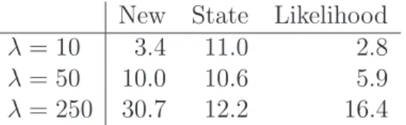
In the first experiment, we generated 100 independent realisations of a homogeneous Poisson process in the unit square for low, medium and high intensity values (λ = 10,50,250). The expected number of points in [0,1]2 is λ. The results are summarised
New State Likelihood
λ= 10 3.4 11.0 2.8
λ= 50 10.0 10.6 5.9
λ= 250 30.7 12.2 16.4
Table 1: Average integrated squared error, divided by the expected number of points, over 100 simulations of a homogeneous Poisson process on the unit square.
5.1.2 Poisson process with linear trend
In the next experiment, we generated 100 independent realisations of a Poisson process in the unit square with intensity function
λ(x, y) = 10 +αx, (x, y)∈[0,1]2,
for weak, medium and strong trend (α = 1,80,480). The expected number of points in [0,1]2 is 10 +α/2. The results are summarised in Table 2.
New State Likelihood
α= 1 4.2 13.0 3.8
α= 80 8.9 11.4 7.4
α= 480 23.0 14.8 17.9
Table 2: Average integrated squared error, divided by the expected number of points, over 100 simulations of a Poisson process with linear trend on the unit square.
5.1.3 Poisson process with modulation
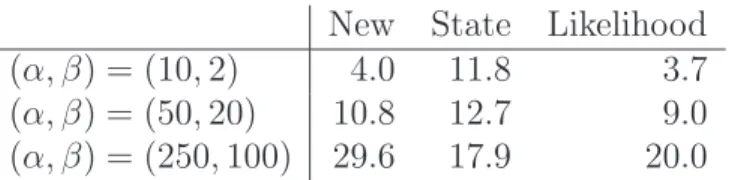
Finally, we generated 100 independent realisations of a Poisson process in the unit square with intensity function
λ(x, y) = α+βcos(10x), (x, y)∈[0,1]2.
To generate patterns with a low, medium and large intensity, we considered the (α, β) combinations (10,2), (50,20) and (250,100). The expected number of points in [0,1]2
is α+βsin(10)/10. The results are summarised in Table 3.
5.2
Cox processes
We next turn to a class of clustered point processes, namely Cox processes (see Sec-tion 2.2). As indicated by the specific experiments below, for each model type consid-ered, the new approach seems to strongly outperform the competing approaches.
New State Likelihood
(α, β) = (10,2) 4.0 11.8 3.7
(α, β) = (50,20) 10.8 12.7 9.0
(α, β) = (250,100) 29.6 17.9 20.0
Table 3: Average integrated squared error, divided by the expected number of points, over 100 simulations of a modulated Poisson process on the unit square.
5.2.1 Homogeneous Mat´ern cluster process
In the first experiment we generated 100 independent realisations of a homogeneous Mat´ern cluster process [7] in the unit square, for various degrees of clustering. This is a Cox process with
Λ(y) = 1
πr2
X
x∈Φ
1{y∈B(x, r)},
where Φ is a homogeneous Poisson process with intensity κ and B(x, r) is the closed ball of radius r, centred at x ∈ R2. In words, each point of Φ acts as a parent to a
family that consists of a Poisson number of offspring (mean sizeµ), born independently of each other at positions that are uniformly distributed in a ball of radius r around the parent. The Mat´ern cluster process Ψ consists of the ensemble of all offspring.
We considered two levels, κ = 10,20, for the parent intensity, two ranges of clus-tering, r = 0.05,0.1, and two mean offspring sizes, µ = 3,10. To avoid edge effects, the parent process was generated on a dilated window. Note that the resulting point process is homogeneous with intensity κµ. As an aside, for general parent intensity functions λ(·), the resulting point process has intensity function
λ(x) = µ
πr2
Z
B(x,y)
λ(u)du.
The results are summarised in Table 4 and we note that the expected number of points in [0,1]2 isκµ. Throughout, the new approach outperforms its competitors. For a low degree of clustering (small values ofµ), the likelihood based method outperforms the state estimation approach; for larger degrees the state estimation method works better. The state estimation and likelihood based methods tend to have decreased integrated squared errors when clusters are more diffuse.
5.2.2 Homogeneous Log-Gaussian Cox process
In the next experiment, we generated 100 independent realisations of a homogeneous Cox process as follows. Let Z be a Gaussian random field with mean zero and covari-ance function
New State Likelihood (κ, r, µ) = (10,0.05,3) 19.5 233.5 158.3 (κ, r, µ) = (10,0.1,3) 15.0 64.5 47.7 (κ, r, µ) = (10,0.05,10) 44.5 627.4 783.9 (κ, r, µ) = (10,0.1,10) 44.2 175.2 214.6 (κ, r, µ) = (20,0.05,3) 22.8 203.8 158.4 (κ, r, µ) = (20,0.1,3) 21.7 58.5 50.6 (κ, r, µ) = (20,0.05,10) 62.9 552.5 765.5 (κ, r, µ) = (20,0.1,10) 71.9 168.9 236.2
Table 4: Average integrated squared error, divided by the expected number of points, over 100 simulations of a homogeneous Mat´ern cluster process on the unit square. Consider further the random measure defined by its intensity
λexp(Z(x, y)).
Then the intensity function of the resulting Cox process, a log-Gaussian Cox process [12, 22], is given by
λexp(σ2/2).
We considered two levels λ = 10,50, two degrees of variability, σ2 = 2 log(5) and σ2 = 2 log(2), as well as two degrees of clustering β = 10,50. Note that the expected
number of points in [0,1]2 is λexp(σ2/2).
The results are summarised in Table 5. As already mentioned, we see that the new approach works the best. It further seems that the likelihood based approach has the second best performance. Increasing β, that is, decreasing the range of interaction, tends to lead to a smaller integrated squared error. Increasing the variability, and hence the intensity, yields a higher integrated squared error.
New State Likelihood
(λ, σ2, β) = (10,2 log(5),50) 14.1 70.8 17.8 (λ, σ2, β) = (10,2 log(2),10) 9.7 28.1 12.4 (λ, σ2, β) = (10,2 log(5),10) 55.0 376.5 208.6 (λ, σ2, β) = (50,2 log(5),50) 73.7 641.7 336.6 (λ, σ2, β) = (50,2 log(2),10) 61.1 130.9 102.2 (λ, σ2, β) = (50,2 log(5),10) 383.4 2,875.1 2,229.9
Table 5: Average integrated squared error, divided by the expected number of points, over 100 simulations of a homogeneous log-Gaussian Cox process.
5.2.3 Log-Gaussian Cox process with linear trend
Turning to the more important scenario of inhomogeneity in combination with cluster-ing, we generated 100 independent realisations of a Cox process as follows. Let Z be the same Gaussian random field as in Section 5.2.2 and consider the random measure defined by its intensity
λ(x, y) exp(Z(x, y)),
whereλ is strictly positive. Then the intensity function of the resulting Cox process is
λ(x, y) exp(σ2/2).
We chose the linear trend function
λ(x, y) = 10 + 80x,
two degrees of variability, σ2 = 2 log(5) and σ2 = 2 log(2), as well as two degrees of
clustering, β = 10,50. Here the expected number of points in [0,1]2 is 50 exp(σ2/2).
The results are summarised in Table 6 and the conclusions, in terms of performance, are the same as for the homogeneous log-Gaussian Cox process in Section 5.2.2.
New State Likelihood
(σ2, β) = (2 log(5),50) 89.6 1477.2 536.0
(σ2, β) = (2 log(2),10) 57.5 136.9 112.6
(σ2, β) = (2 log(5),10) 335.3 2,960.6 2,251.2
Table 6: Average integrated squared error, divided by the expected number of points, over 100 simulations of a log-Gaussian Cox process with linear trend.
5.2.4 Log-Gaussian Cox process with modulation
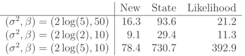
In the next experiment, we generated 100 independent realisations of a Cox process in the same way as in Section 5.2.3, but with
λ(x, y) = 10 + 2 cos(10x).
Here we used two degrees of variability, σ2 = 2 log(5) and σ2 = 2 log(2), as well as
two degrees of clustering, β = 10,50. The expected number of points in [0,1]2 is
(10 + sin(10)/5) exp(σ2/2).
The results are summarised in Table 7. Also here the conclusions are the same. The selection (15) is performing the best and the state estimation approach the worst, with increasingβ leading to a smaller integrated squared error and increased variability yielding a higher integrated squared error.
New State Likelihood (σ2, β) = (2 log(5),50) 16.3 93.6 21.2
(σ2, β) = (2 log(2),10) 9.1 29.4 11.3
(σ2, β) = (2 log(5),10) 78.4 730.7 392.9
Table 7: Average integrated squared error, divided by the expected number of points, over 100 simulations of a modulated log-Gaussian Cox process.
5.3
Determinantal point processes
We finally turn to planar determinantal point processes (see e.g. [16]). Such processes exhibit inhibition/regularity and allow explicit expressions for the product densities
ρ(n)((x
1, y1), . . . ,(xn, yn)) = det(C((xi, yi),(xj, yj)))i,j, (xi, yi)∈R2,
in terms of a kernelC. Here det denotes the determinant operator. Hence, the intensity function is given by λ(x, y) =ρ(1)(x, y) = C((x, y),(x, y)). Throughout, we will use
C((x1, y1),(x2, y2)) =σ2exp(−βk(x1, y1)−(x2, y2)k)
as basis, resulting in a homogeneous determinantal point process with intensity
λ(x, y) =C((x, y),(x, y)) =σ2.
Hence, the expected number of points in [0,1]2 isσ2. 5.3.1 Homogeneous determinantal point process
We generated 100 independent realisations of the homogeneous model above, on the unit square, for low, medium and high intensity values (σ2 = 10,50,250). We further
considered two values for β, namely 20 and 50. For σ2 = 250, the model is not valid
for the larger of the interaction ranges, that is, for β = 20. To alleviate edge effects, we considered realisations on a dilated window of size 2/β, which was restricted to the unit square.
The results, which are summarised in Table 8, indicate that for small intensities the likelihood based method performs the best and the state estimation approach generates the highest average integrated squared error. For medium intensities the likelihood based approach performs the best, with the other two approaches giving rise to similar average integrated squared errors. In the case of high intensities, the state estimation method performs the best and the new method gives rise to the highest average integrated squared error.
New State Likelihood (σ2, β) = (10,50) 4.0 11.0 3.2 (σ2, β) = (10,20) 4.1 13.1 3.2 (σ2, β) = (50,50) 10.9 10.6 6.3 (σ2, β) = (50,20) 9.6 8.4 4.8 (σ2, β) = (250,50) 27.6 10.4 11.7
Table 8: Average integrated squared error, divided by the expected number of points, over 100 simulations of a homogeneous determinantal point process.
5.3.2 Determinantal point process with linear trend
Next, we applied independent thinning (see e.g. [7]) to the realisations of the ho-mogeneous determinantal point process described above. We employed the retention probabilities
p(x, y) = 10 + 80x
90 , (x, y)∈[0,1]
2,
which results in the intensity being given by λ(x, y) = σ2p(x, y). We considered the
cases λ = 50,250 and β = 20,50. The results are summarised in Table 9. Here, the expected number of points in [0,1]2 is 5σ2/9. We found indications that in the low and
medium intensity cases the likelihood based approach performs the best, followed by the new approach. On the other hand, in the high intensity setting the likelihood based approach and the state estimation approach seem to perform almost equally well.
New State Likelihood (σ2, β) = (50,50) 7.0 10.6 5.3
(σ2, β) = (50,20) 6.2 9.7 5.1
(σ2, β) = (250,50) 16.7 10.8 10.9
Table 9: Average integrated squared error, divided by the expected number of points, over 100 simulations of a determinantal point process with linear trend.
5.3.3 Determinantal point process with modulation
In the last experiment, we applied independent thinning to realisations of the homo-geneous determinantal point process described in the previous section, using retention probabilities
p(x, y) = 10 + 2 cos(10x)
12 , (x, y)∈[0,1]
2,
for λ = 10,50 and β = 20,50. Note that the expected number of points in [0,1]2
intensity, the new approach and the likelihood based approach seem to have similar, but also the best, performance. As we increase the intensity, the new approach tends to generate a higher average integrated squared error than the likelihood based approach. The state estimation method tends to perform poorly for small intensities; there may not be enough points to reliably estimate the K-function in (11) and (12).
New State Likelihood (σ2, β) = (10,50) 4.0 11.7 4.9
(σ2, β) = (10,20) 3.7 13.2 3.3
(σ2, β) = (50,50) 9.8 10.6 6.4
(σ2, β) = (50,20) 8.5 8.4 4.8
Table 10: Average integrated squared error, divided by the expected number of points, over 100 simulations of a modulated determinantal point process.
6
Discussion
We have proposed a new approach for the selection of bandwidth h > 0 in a kernel estimator bλ(x;h,Ψ, W) of the intensity function λ(x) >0, x∈ W, of a point process Ψ. The basic idea is to minimise the discrepancy between the size of the study re-gion, ℓ(W), and the sum of reciprocals Tκ(h; Ψ, W) = Px∈Ψ∩Wbλ(x;h,Ψ, W)−1. Our
approach is mandated by the fact that replacing bλ(x;h,Ψ, W) by λ(x) in Tκ(h; Ψ, W)
turns this statistic into an unbiased estimator of ℓ(W). In essence, we have trans-formed the problem of selecting the unknown optimal bandwidth to that of estimating the known size of the study region and, as a by-product, we obtain an estimate of the optimal bandwidth. Our approach, being based solely on the general Campbell theo-rem (1), is fully non-model based, as opposed to the current state of the art methods. These approaches, the Poisson process likelihood cross-validation approach [2, 20] and the state estimation approach [11], both assume that the underlying point process Ψ is of a given model class.
The results of the simulation study carried out in this paper suggest the following tentative conclusions. For clustered patterns, the new method appears to be the best choice. For Poisson processes, at least for moderately sized patterns, the likelihood based cross-validation method seems to give the best results. The picture is a bit more varied for regular patterns. Broadly speaking, both the new method and the likelihood based method give good results for low and moderate intensity values; the state estimation method seems best for dense patterns. Indeed, there are indications that the state estimation approach outperforms the other methods when the intensity becomes very large. Finally, in terms of computational speed, the state estimation ap-proach is the fastest of the methods considered in this paper and the Poisson likelihood
cross-validation approach is the slowest.
Taking these observations into consideration, we tentatively suggest using the new approach, unless i) the pattern exhibits clear inhibition/regularity, or ii) the number of points is very large and the pattern clearly exhibits no clustering. When i) holds we suggest employing the likelihood based approach and when ii) holds one should consider the state estimation approach.
The method proposed in Section 4 assumes that the intensity function is strictly positive. However, it is not hard to deal with any zero or near-zero intensity regions that may arise in practice by a simple superposition. More specifically, consider a further point process Ξ⊆ W that is independent of Ψ, with known intensity function
λΞ(x)>0. Then the superposition Ψ∪Ξ has intensity [7, p. 165]
λΨ∪Ξ(x) =λ(x) +λΞ(x), x∈W,
which is strictly positive. By employing (15) to obtain an estimate bλΨ∪Ξ(·;h) based on
(Ψ∪Ξ)∩W, we may subtract the known intensity λΞ(·) to obtain the final estimate
b
λ(·;h). Some care must be taken when choosing Ξ. IfλΞis too small, the superposition will not help in solving the numerical problem of having near-zero intensities. However, if λΞ is too large, the features of Ψ may not be detectable through Ψ∪Ξ. Note that in practise the execution amounts to repeating this procedure for a large number of simulations of Ξ.
It may be noted that (15) can be expressed as a general intensity estimation crite-rion. More specifically, given some collection Γ of functions γ :E →(0,∞), which are estimating the underlying intensityλ(·), one would use as estimatebλ(·) a minimiser of
F(γ) = (Px∈Ψ∩Wγ(x)−1−ℓ(W))2,γ ∈Γ. In fact, this is a way of estimating marginal
Radon-Nikodym derivatives, without explicit knowledge of the multivariate structures. This bring us to our ongoing work, where we explore, among other things, estimation of higher order product densities, adaptive kernel estimation, intensity estimation for marked and/or spatio-temporal point processes, as well as parametric estimation.
Appendix: Proof of Lemma 1
First note that the κγ, as defined in (6), are continuous functions for γ > 0, as is
the Gaussian kernel (7). The function h → 1/h is continuous on the open inter-val (0,∞), whereby the composition h → κγ(x/h) is also continuous in h on (0,∞).
As for the local and global edge correction functions, by the dominated convergence theorem, using the fact that W and κγ are bounded, also w
h(x, y) is continuous in
h; moreover, it takes strictly positive values since W is open. Therefore, bλ(x;h) is also continuous in h on (0,∞). Finally, since for x ∈ Ψ∩W, the kernel estima-tor λb(x;h) ≥ h−dκγ(0)/w
continuous in h ∈ (0,∞). Box kernels are discontinuous at 1, making Tκ0 piecewise
continuous.
Now let htend to zero. For the Beta kernels with γ ≥0, the support ofh−dκγ((· −
y)/h) is the ball centred at y with radius h. Since the volume of such a ball tends to zero as h tends to zero and W is open, using the fact that κγ is a symmetric
probability density, we obtain that limh→0wh(x, y) = 1 for allx, y ∈W for global and
local edge correction. This holds trivially if no edge correction is applied. For the Gaussian kernel, note thath−dκ((· −y)/h) corresponds to the probability density ofd
independent normally distributed random variables with standard deviationh centred at the components ofy/h. Take a sequencehn→0 and writeXnfor the corresponding
Gaussian random vector. Then Xn converges in distribution to the Dirac mass at y
by L´evy’s continuity theorem. Since W is open, it is a continuity set, and wh tends to
1 for local edge correction. The global case follows from the symmetry of κ and the case wh ≡1 is trivial. Note that for all considered kernels, 0≤κ(·)≤κ(0). Forx=y
and all h > 0, κ((x−y)/h) =κ(0). Therefore, having excluded the pathological case that Ψ∩W is empty, Py∈Ψ∩Wκ((x−y)/h)wh−1(x, y)≥ κ(0)w−h1(x, x) which tends to
κ(0)>0 ash→0. Observing thathd tends to zero withh, we obtain the desired limit
limh→0Tκ(h; Ψ, W) = 0.
Next, let h tend to infinity. Since κ(·)≤ κ(0), limh→∞h−dκ((x−y)/h) = 0 for all
x, y ∈ W. Therefore, Tκ(h; Ψ, W) tends to infinity when wh ≡ 1 and Ψ∩W 6= ∅. If
one does correct for edge effects, by the continuity of κ in 0 for all considered kernels,
κ((x−y)/h) tends to κ(0) as h → ∞. Furthermore, since W is bounded, by the dominated convergence theorem,
Z
W
κ((x−u)/h)du→κ(0)ℓ(W).
Upon using the symmetry ofκ, we obtain that for both local and global edge correction,
hdw
h(x, y)→κ(0)ℓ(W). Thereforebλ(x;h)→ |Ψ∩W|/ℓ(W) and limh→0Tκ(h; Ψ, W) =
ℓ(W). This completes the proof.
References
[1] Baddeley, A.J., Møller, J., Waagepetersen, R. (2000). Non- and semi-parametric estimation of interaction in inhomogeneous point patterns. Statistica Neerlandica 54:329–350.
[2] Baddeley, A., Rubak, E., Turner, R. (2016). Spatial Point Patterns. Methodology and Applications with R. Boca Raton: Taylor & Francis/CRC Press.
[3] Barr, C.D., Schoenberg, F.P. (2010). On the Voronoi estimator for the intensity of an inhomogeneous planar Poisson process. Biometrika 97977–984.
[4] Berman, M., Diggle, P.J. (1989). Estimating weighted integrals of the second-order intensity of a spatial point process. Journal of the Royal Statistical Society, Series B 51:81–92.
[5] Bernardeau, F., Weygaert, R. van de (1996). A new method for accurate estima-tion of velocity field statistics. Monthly Notices of the Royal Astronomical Society 279:693–711.
[6] Bowman, A.W., Azzalini, A. (1997).Applied Smoothing Techniques for Data Anal-ysis: The Kernel Approach with S-Plus Illustrations. Oxford: Clarendon Press. [7] Chiu, S.N., Stoyan, D., Kendall, W.S., Mecke, J. (2013).Stochastic Geometry and
its Applications, 3rd Edition. Chichester: Wiley.
[8] Cronie, O., Lieshout, M.N.M. van (2016). Summary statistics for inhomogeneous marked point processes.Annals of the Institute of Statistical Mathematics 68:905– 928.
[9] Daley, D.J., Vere-Jones, D. (2008). An Introduction to the Theory of Point Pro-cesses: Volume II: General Theory and Structure. Second Edition. New York. Springer.
[10] Davies, L. (2014). Data Analysis and Approximate Models. Model Choice, Location-Scale, Analysis of Variance, Nonparametric Regression and Image Anal-ysis. Boca Raton: Taylor & Francis/CRC Press.
[11] Diggle, P.J. (1985). A kernel method for smoothing point process data. Applied Statistics 34:138–147.
[12] Diggle, P.J. (2014).Statistical Analysis of Spatial and Spatio-Temporal Point Pat-terns. Third Edition. Boca Raton: Taylor & Francis/CRC Press.
[13] Gelfand, A.E., Diggle, P.J., Fuentes, M., Guttorp, P. (Eds.) (2010). Handbook of Spatial Statistics. Boca Raton: Taylor & Francis/CRC Press.
[14] Hall, P., Minnotte, M.C., Zhang, C. (2004). Bump Hunting With Non-Gaussian Kernels. The Annals of Statistics 32:2124–2141.
[15] Illian, J., Penttinen, A., Stoyan, H., Stoyan, D. (2008). Statistical Analysis and Modelling of Spatial Point Patterns. Chichester: Wiley.
[16] Lavancier, F., Møller, J., Rubak, E. (2015). Determinantal point process models and statistical inference. Journal of the Royal Statistical Society, Series B 77: 853–877.
[17] Lieshout, M.N.M. van (2000). Markov Point Processes and Their Applications. London/Singapore: Imperial College Press/World Scientific.
[18] Lieshout, M.N.M. van (2011). A J-function for inhomogeneous point processes. Statistica Neerlandica 65:183–201.
[19] Lieshout, M.N.M. van (2012). On estimation of the intensity function of a point process. Methodology and Computing in Applied Probability 14:567–578.
[20] Loader, C. (1999). Local Regression and Likelihood. New York: Springer.
[21] Matthes, K., Kerstan, J., Mecke, J. (1978). Infinitely Divisible Point Processes. Chichester: Wiley.
[22] Møller, J., Syversveen, A., Waagepetersen, R. (1998). Log Gaussian Cox Processes. Scandinavian Journal of Statistics 25:451–482.
[23] Ogata, Y. (1998). Space-time point process models for earthquake occurrences. Annals of the Institute of Statistical Mathematics 50:379–402.
[24] Ord, J.K. (1978). How many trees in a forest? Mathematical Sciences 3:23–33. [25] Schaap, W.E. (2007). DTFE. The Delaunay Tessellation Field Estimator. Ph.D.
Thesis, University of Groningen.
[26] Schaap, W.E., Weygaert, R. van de (2000). Letter to the Editor. Continuous fields and discrete samples: Reconstruction through Delaunay Tessellations. Astronomy and Astrophysics 363:L29–L32.
[27] Scott, D.W. (1992). Multivariate Density Estimation. Theory, Practice and Visu-alization. New York: Wiley.
[28] Silverman, B.W. (1986). Density Estimation for Statistics and Data Analysis. London: Chapman & Hall.