PROOFS PRODUCED BY SECONDARY SCHOOL STUDENTS LEARNING GEOMETRY IN A DYNAMIC COMPUTER
ENVIRONMENT
ABSTRACT. As a key objective, secondary school mathematics teachers seek to improve the proof skills of students. In this paper we present an analytic framework to describe and analyze students’ answers to proof problems. We employ this framework to investigate ways in which dynamic geometry software can be used to improve students’ understanding of the nature of mathematical proof and to improve their proof skills. We present the results of two case studies where secondary school students worked with Cabri-Géomètre to solve geometry problems structured in a teaching unit. The teaching unit had the aims of: i) Teaching geometric concepts and properties, and ii) helping students to improve their con-ception of the nature of mathematical proof and to improve their proof skills. By applying the framework defined here, we analyze students’ answers to proof problems, observe the types of justifications produced, and verify the usefulness of learning in dynamic geometry computer environments to improve students’ proof skills.
KEY WORDS: Cabri, Dynamic geometry software, Computer learning environment, Geo-metry, Justification, Proof, Secondary school, Teaching experiment
1. INTRODUCTION
One of the most interesting and difficult research fields in mathematics education concerns how both to help students come to a proper understand-ing of mathematical proof and enhance their proof techniques. Over past decades, numerous researchers have experimented with different forms of teaching. Generally, we can say that their attempts to teach formal mathematical proof to secondary school students (frequently during short periods of time) were not successful (Clements and Battista, 1992). This observation coheres with Senk’s research (1989) on the van Hiele model. She shows that most students who finish secondary school achieve only the first or second van Hiele level, and that progress from the second to the fourth level is very slow. Generally, it takes several years for students to reach level four from level two.
The work of Bell (1976a) and De Villiers (1990 and 1996) has led to general agreement on the main objectives of mathematical proof: To verify or justify the correctness of a statement, to illuminate or explain
Educational Studies in Mathematics 44: 87–125, 2000.
why a statement is true, to systematize results obtained in a deductive sys-tem (a syssys-tem of axioms, definitions, accepted theorems, etc.), to discover new theorems, to communicate or transmit mathematical knowledge, and to provide intellectual challenge to the author of a proof. However, stu-dents rarely identify with any of these objectives. We vitally need to know students’ conception of mathematical proof in order to understand their attempts to solve proof problems.1That is, we need to know what it is for them to ‘prove’ a statement or, in other words, what kind of arguments convince students that a statement is true. This knowledge can then be put to use in teaching a conception of mathematical proof that comes closer to the conception currently accepted by mathematicians.
Along this line, the approach of mathematics education researchers to this topic has changed during recent years: The goal of educational research is no longer attempting to find ways to promote skill in formal mathematical proof, but to study the evolution of the students’ understand-ing of mathematical proof and to find out how to help them improve their understanding. This change of goals arises in part from the general convic-tion that secondary school students are not able to begin an apprenticeship in methods of formal proof suddenly, as has sometimes been attempted (Senk, 1985; Serra, 1989). Instead apprenticeship in the methods of formal proof should be considered the last step along a long road.
Several authors have observed, from different points of view, students as they attempt to solve proof problems. Some authors have described types of students’ justifications. Others have analyzed the ways in which students produce justifications, including the ways in which they produce conjectures when required. A complete assessment of students’ justifica-tion skills has to take into considerajustifica-tion both products (i.e., justificajustifica-tions produced by students) and processes (i.e., the ways in which students pro-duce their justifications). In section 2 of this paper we describe the main results of previous research and integrate these results into a wider frame-work which considers both the ways in which students produce conjectures and justifications, and the resulting justification itself.
Modern dynamic geometry software (DGS) has stimulated research on students’ conceptions of proof by opening up new directions for this research to take. The contribution of DGS is two-fold. First, it provides an environment in which students can experiment freely. They can easily check their intuitions and conjectures in the process of looking for pat-terns, general properties, etc. Second, DGS provides non-traditional ways for students to learn and understand mathematical concepts and methods. These ways of learning pose many questions that mathematics education researchers should investigate.
In section 3 we describe an experiment in which secondary school geo-metry was taught using Cabri-Géomètre (Baulac, Bellemain and Laborde, 1988). Cabri was used in the 30 activities of the teaching unit. In section 4 we report on two case studies of two pairs of students. Our analysis of the solutions of both pairs and of their responses during clinical interviews show that each pair differed from the other in how the same proof problems were solved. Finally, section 5 summarizes the main hypothesis of our study and its conclusions, and raises some issues for future research.
Terms such as explanation, verification, justification, and proof have been used in the literature to refer, in one way or another, to convincing a speaker, or oneself, of the truth of a mathematical statement. Sometimes the same term carries more than one meaning (see, for example, the mean-ings of ‘justification’ in Bell, 1976a; Balacheff, 1988a; Hanna, 1995). This issue is beyond the scope of this paper. From now on in this paper, we will use the term justificationto refer to any reason given to convince people (e.g., teachers and other students) of the truth of a statement, and we will use the term (formal mathematical)proofto refer to any justification which satisfies the requirements of abstraction, rigor, language, etc., demanded by professional mathematicians to accept a mathematical statement as valid within an axiomatic system.
2. IDENTIFICATION OF AN ANALYTIC FRAMEWORK
There are many studies dealing with the processes by which students learn to justify mathematical statements. Some of these studies develop inter-esting, if partial, methods of analyzing the processes. These methods fit into two main categories: Descriptions of forms of students’ work when solving proof problems (Arzarello et al., 1998a; Balacheff, 1988a and b; Bell, 1976a and b; Harel and Sowder, 1996; Sowder and Harel, 1998), and descriptions of students’ beliefs when deciding whether they are convinced by an argument about the truth of a statement, or not (De Villiers, 1991; Harel and Sowder, 1996; Sowder and Harel, 1998). Our study follows the first approach. In the second part of this section we describe an integrated framework which we later use to study students’ attempts to solve proof problems. This framework provides a way to analyze and classify the pro-cesses of coming up with conjectures (when required by the problem) and of producing justifications, as well as analyzing and classifying the justifications themselves.
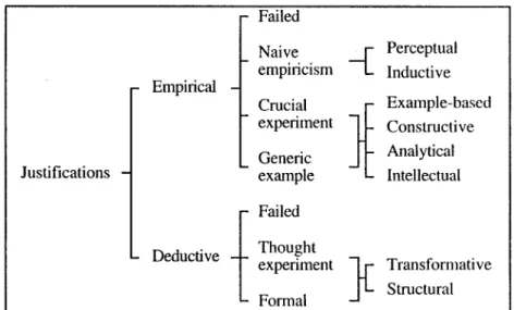
Bell (1976a and b) identified two categories of students’ justifications used in proof problems:Empiricaljustification, characterized by the use of examples as element of conviction, anddeductivejustification,
character-ized by the use of deduction to connect data with conclusions. Within each category, Bell identified a variety of types: The types of empirical answers correspond to different degrees of completeness of checking the state-ment in the whole (finite) set of possible examples. The types of deductive answers correspond to different degrees of completeness of constructing deductive arguments.
Balacheff (1988b) distinguished between two categories of justifica-tion, which he called pragmatic and conceptual justifications. Pragmatic justifications are based on the use of examples, or on actions or showings, and conceptual justifications are based on abstract formulations of prop-erties and of relationships among propprop-erties. The category of pragmatic justifications includes three types:Naive empiricism, in which a statement to be proved is checked in a few (somewhat randomly chosen) examples; crucial experiment, in which a statement is checked in a careful selected example; andgeneric example, in which the justification is based on opera-tions or transformaopera-tions on an example which is selected as a characteristic representative of a class. In this case, operations or transformations on the example are intended to be made on the whole class. The category of conceptual justifications includesthought experiment, in which actions are internalized and dissociated from the specific examples considered, and symbolic calculationsfrom the statement, in which there is no experiment and the justification is based on the use of and transformation of formalized symbolic expressions.
Harel and Sowder (1996), and Sowder and Harel (1998) identified three categories of justifications (labelledproof schemes):Externally based, when the justification is based on the authority of a source external to students, like teacher, textbook, etc.;empirical, when the justification is based solely on examples (inductive type) or, more specifically, drawings (perceptual type), analyticalor theoretical, when the justification is based on generic arguments or mental operations that result in, or may result in, formal mathematical proofs. Such arguments or operations can be based on gen-eral aspects of a problem (transformational type) or contain different re-lated situations, resulting in deductive chains based on elements of an axiomatic system (structural or axiomatic type).
The above categories describe students’ outcomes (justifications) but they do not consider the process of production of such outcomes. Fur-thermore, the focus of each study was different from that of the other studies, and each study was partial: With regard to the empirical/pragmatic categories, Bell analyzed only the completeness of sets of examples used by students; Balacheff focused on students’ reasons for selecting examples and on how they used them; and Sowder and Harel differentiated
justific-ations based only on visual or tactile perception and on the observation of mathematical properties.
Among the deductive/conceptual/analytical categories, those defined by Bell differ in the mathematical quality of their deductive chains. Sowder and Harel described two types of analytical justifications, one based on transforming the conditions of the problem, and the other based on the use of elements of an axiomatic system. Balacheff identified only a type of conceptual justifications (those which take into account specific examples but are not based on them as elements of conviction) and justifications through symbolic calculations.
To promote progress in the description and understanding of students’ answers to proof problems, we have defined a three-faceted classification scheme in which all of the student’s activity – generation of a conjecture (if required), devising a justification, and the resulting justification – is considered:
1) Like Bell, Balacheff, and Sowder and Harel, we have differentiated between two main categories, empirical and deductive justifications, depending on whether the justificationconsists of checking examples, or not.
2) Empirical justifications have been split into several subclasses de-pending on the ways students select examples to be used in their justifications, and each subclass has several types corresponding to distinctways students usethe selected examples in their justifications. 3) Deductive justifications have been split into two subclasses depend-ing on whether students select an example, or not, to help organize their justification, and each subclass has been divided into two types depending on thestyles of deductionmade to organize justifications. The whole classification scheme is as follows:
* Empirical justifications, characterized by the use of examples as the main (maybe the only) element of conviction: Students state conjectures after having observed regularities in one or more examples; they use the examples, or relationships observed in them, to justify the truth of their conjecture. When the conjecture is included in the statement of a prob-lem, students have only to construct examples to check the conjecture and justify it. Within empirical justifications, we distinguish three classes, depending on the way examples are selected:
– Naive empiricism, when the conjecture is justified by showing that it is true in one or several examples, usually selected without a spe-cific criterion. The checking may involve visual or tactile perception of examples only (perceptual type) or may also involve the use of
mathematical elements or relationships found in examples (inductive type).
– Crucial experiment, when the conjecture is justified by showing that it is true in a specific, carefully selected, example. Students are aware of the need for generalization, so they choose the example as non-particular as possible (Balacheff, 1987), although it is not considered as a representative of any other example. Students assume that the conjecture is always true if it is true in this example. We distinguish several types of justifications by crucial experiment, depending on how the crucial example is used:
Example-based, when the justification shows only the existence of an example or the lack of counter-examples; constructive, in which the justification focuses on the way of getting the example; analytical, in which the justification is based on properties empirically observed in the example or in auxiliary elements; and intellectual, when the justification is based on empirical observation of the example, but the justification mainly uses accepted properties or relationships among elements of the example. Intellectual justifications show some decon-textualization (Balacheff, 1988b), since they include deductive parts in addition to arguments based on the example.
The main difference between analytical and intellectual justifications is the source of properties or relationships referred to: In analytical justifications they are originated by the empirical observation of ex-amples (for instance, a student makes some measurements on an equi-lateral triangle and he/she notes that an angle bisector bisects the opposite side), while in intellectual justifications the empirical ob-servation induces the student to remember a property that had been learned before (for instance, the student makes the same measure-ments on an equilateral triangle and he/she remembers that its angle bisectors are also its medians).
The two main differences between a crucial experiment and naive empiricism are i) the status of the specific example, and ii) that an example used in a crucial experiment has been selected to be repres-entative of a certain class.
– Generic example, when the justification is based on a specific ex-ample, seen as a characteristic representative of its class, and the justification includes making explicit abstract reasons for the truth of a conjecture by means of operations or transformations on the ex-ample. The justification refers to abstract properties and elements of a family, but it is clearly based on the example. The four types of jus-tifications (example-based, constructive, analytical and intellectual)
defined for the crucial experiment are found here too, in descriptions of how the generic example is used in the justification.
The main difference between a crucial experiment and a generic ex-ample is that, in a crucial experiment, justification consists only of experimental verification of the conjecture in the selected example while, in a generic example, justification includes references to ab-stract elements or properties of the class represented by the example. – Failedanswer, when students use empirical strategies to solve a proof problem but they do not succeed in elaborating a correct conjecture or they do state a correct conjecture but they do not succeed in providing any justification.
* Deductive justifications, characterized by the decontextualization of the arguments used, are based on generic aspects of the problem, mental oper-ations, and logical deductions, all of which aim to validate the conjecture in a general way. Examples, when used, are a help to organize arguments, but the particular characteristics of an example are not considered in the justification. Within deductive justifications, we distinguish three classes:
– Thought experiment, when a specific example is used to help organ-ize the justification. Sometimes a thought experiment has a temporal development (Balacheff, 1988b), as a consequence of the observa-tion of the example, and it refers to acobserva-tions, but these are internal-ized and detached from the example. Following Harel and Sowder (1996), we can find two types of thought experiments, depending on the style of the justification:Transformativejustifications are based on mental operations producing a transformation of the initial problem into another equivalent one. The role of examples is to help foresee which transformations are convenient. Transformations may be based on spatial mental images, symbolic manipulations or construction of objects. Structuraljustifications are sequences of logical deductions derived from the data of the problem and axioms, definitions or ac-cepted theorems. The role of examples is to help organize the steps in deductions.
– Formal deduction, when the justification is based on mental opera-tions without the help of specific examples. In a formal deduction only generic aspects of the discussed problem are mentioned. It is, therefore, the kind of formal mathematical proof found in the world of mathematics researchers. We may also find the two types of justi-fications (transformative and structural) defined in the previous para-graph.
– Failed, when students use deductive strategies to solve proof prob-lems but they do not succeed in elaborating a correct conjecture or
Figure 1. Types of justification.
they elaborate a correct conjecture but they fail in providing a justi-fication.
Figure 1 summarizes previous types of justifications. This classification is detailed enough to make a fine discrimination among a student’s answers to different problems. The two types of failed justifications are necessary to complete the classification because the assessment of students’ justi-fication and proof skills cannot be associated only to correct solutions of problems. Apart from classifying students’ answers, this classification scheme is useful to evaluate the improvement of a student’s justification skills in a learning period. The use of this classification to analyze data from our teaching experiment allowed us to evaluate changes in students’ justification skills. Another application of this classification scheme could be to observe the possible influence of peculiarities of a specific envir-onment on students’ learning; for instance, it has been argued that DGS environments tend to promote some types of empirical justifications and inhibit formal justifications (Chazan, 1993; Healy, 2000).
The different classifications of justifications described in this section, including ours, implicitly assume that students work in a coherent linear way from beginning to end of the solution of a problem. However, the reality is, in many cases, different. Typically, many students begin by using empirical checking and, when they have understood the problem and the way to justify the conjecture, they continue by writing a deductive justi-fication. It is also usual to make several jumps among deductive and
em-pirical methods during the solution of a problem. Arzarello et al. (1998a) considered these cases by analyzing the solution of problems paying spe-cial attention to the moment when the solver moves from an ascending phase, characterized by an empirical activity aiming to better understand the problem, generate a conjecture, or verify it, to a descending phase, where the solver tries to build a deductive justification. When solving complex proof problems, often students move forth and back between both phases. Therefore, these researchers’ proposal is to observe and analyze the whole process of solution of proof problems, including early steps toward identification of a conjecture or the finding of a justification. An application of this construct to students working in a Cabri environment can be seen in Arzarello et al. (1998b). By merging the model proposed in Arzarello et al. (1998a) with the classification scheme defined above (Figure 1), we get a framework with two appraisal viewpoints to analyze solutions to proof problems, where one of them corresponds to types of justification produced by students, and the other to shifts among empirical and deductive methods taking place during the process of solution of prob-lems. In this way both the solution to a problem and the process of working out such solution are analyzed together.
3. THE STUDY
The study reported here consisted in the design of a geometry teaching unit based on Cabri, its implementation in a mathematics class, and the observation of students. In this paper we present the observation of two pairs of students. The main objective of the study was to investigate how DGS environments can help students improve their conception of proof in mathematics and their methods of justification.
DGS helps teachers create learning environments where students can experiment, observe the permanence, or lack of permanence, of mathem-atical properties, and state or verify conjectures much more easily than in other computational environments or in the more traditional setting of paper and pencil. The main advantage of DGS learning environments over other (computational or non-computational) environments is that students can construct complex figures and can easily perform in real time a very wide range of transformations on those figures, so students have access to a variety of examples that can hardly be matched by non-computational or static computational environments. A hypothesis of this study is that the Cabri environment we have designed is more helpful than an environment based on non-computer didactical tools or on the traditional
blackboard-and-textbook, because the Cabri environment favours classroom organiza-tion to promote active methodologies.
The use of DGS to help students improve their ways of justificating or proving in mathematics is controversial. Its supporters underline its multiple virtues as facilitator of learning and understanding (De Villiers, 1998). On the other side, some researchers warn against the possibility that these environments may impede student’s leaving empirical justifications to learn more formal methods of proof, because it is so easy to make use of exhaustive checking on the screen that many students become convinced of the truth of conjectures and do not feel the necessity of more abstract justifications (Chazan, 1993; Healy, 2000). In such cases, the teacher’s role is to help them go beyond, since research shows that an adequate planning of activities in a DGS environment can help students produce abstract deductive justifications or, in particular, proofs (Mariotti et al., 1997; Mariotti, this issue). Another hypothesis of our study is that the Cabri environment we have designed does not impede the improvement of students’ justification skills. On the contrary, this DGS environment may help students use different types of justification, setting the basis for them to move from the use of basic to more complex types of empirical justifications, or even to deductive ones, as reflected by a change in the types of justifications produced in the experiment, and by a more coherent oscillation between ascending and descending phases.
In most research on teaching in DGS environments, participant students were novice users of the software, so part of the time in those experiments was devoted to teaching them how to use the software. Furthermore, stu-dents’ lack of experience in the use of software caused many of them to use wrong strategies to solve problems, or strategies more naive than what would have been used in a more familiar environment. We have eliminated this possible limitation from our study, because participant students had used Cabri over several months in the previous academic year, so they were knowledgeable of the software, and they understood the meaning of the actions to be accomplished with Cabri (dragging, modification of objects, etc.). They also understood the difference between a figure as an object characterized by mathematical properties implicit in commands used for its construction, and adrawingas a particular representation of a figure on the screen2(Parzysz, 1988; Laborde and Capponi, 1994).
3.1. Sample
A group of 16 students in their 4th grade of Secondary School (aged 15– 16 years) participated in the teaching experiment. It was carried out as part of the ordinary mathematics teaching, with their own teacher (one
of the researchers and authors) and during the standard class time. The classroom had a set of PC computers with Cabri-Géomètre (version 1.7). Students worked in pairs. This group of students had the same math teacher the year before, when they began to work with Cabri to solve conjecture problems, so the teaching experiment could be organized on the basis of their experience and knowledge gained during the previous year.
Two pairs of students were selected by the teacher before beginning the experiment for follow-up in this case study. These four students, all boys, represented abilities and attitudes from high to average. One of them was the best in the class and the other three were average (it was decided not to include students whose reasoning skills were judged to be very poor, so meaningful data collection would most probably not be possible).
3.2. The teaching experiment
This teaching unit was part of the normal content of the course, and stu-dents need to pass an exam at the end of the course. The teaching unit had as main objectives:
– To facilitate the teaching of concepts, properties and methods usually found in the school plane geometry curriculum: Straight lines and angles among them. Properties and elements of triangles (perpen-dicular bisectors, angle bisectors, etc.). Congruence and similarity of triangles. Relationships among angles and/or other elements of a triangle. Quadrilaterals, their properties and elements. Classifications of triangles and quadrilaterals. Circles, angles and tangents.
– To facilitate a better understanding by students of the need for and function of justifications in mathematics.
– To facilitate and induce the progress of students toward types of jus-tification closer to formal mathematical proofs. In terms of van Hiele levels, with respect to justifications, the objective was to help students to do, by the end of the experiment, justifications in, at least, the third level.
The teaching unit had 30 activities. Each activity was structured in several phases, beginning with a phase where students had to create a figure in Cabri and explore it (in a few activities the figure was provided by the teacher in a file to be opened by the students). In the second phase students had to generate conjectures (in some activities, the students were asked only to check a given conjecture). In the last phase students had to justify conjectures they had stated (some activities did not include this phase). The aim of activities 1 to 11, 14, and 22 was to teach several geometry concepts necessary, as previous knowledge, to solve activities 12 to 30.
Those activities did not include the phase of justification of conjectures. Annex 1 includes summarized information about the activities. Each activ-ity was presented to the students in a worksheet where they had to write their observations, comments, conjectures and justifications.
The activities were conceived in an endeavor to get maximum benefit from the dynamic capability of Cabri. As usual in most Cabri environ-ments, in this teaching unit dragging had a central role in the generation and checking of conjectures: As part of the didactical contract present in the teaching experiment, the ‘dragging test’ acquired the status of an essen-tial element to check the validity of a construction, since students verified that a figure was correct because it passed the dragging test, i.e. they could not mess the figure up by dragging (Noss et al., 1994). Furthermore, drag-ging was a very helpful tool for students when they had to check or state conjectures (they could easily recognize regularities that they identified as mathematical properties) and to make empirical justifications. Many activities would have been too difficult for these students if stated in a paper-and-pencil environment, because they could only be solved by using deductive reasoning far from most students’ capability (e.g., activity 20; see section 4.2). Other activities could not have been solved with paper and pencil by any student (e.g., construction 1 in activity 30; see section 4.3) because they lacked the necessary knowledge of geometrical facts and relationships, and abstract reasoning ability.
Dragging was sufficient to convince most pupils of the correctness of conjectures, so questions like ‘why is the construction valid?’ or ‘why is the conjecture true?’ were important to induce students to elaborate jus-tifications beyond the simple checking of some examples on the screen by dragging. As part of the didactical contract defined in the class, pupils knew that requirements like ‘justify your conjecture’ carried the implicit meaning of ‘justify why your conjecture or construction is true’.
Two 55-minute mathematics classes per week were devoted to the teach-ing experiment. Students worked on each activity durteach-ing two consecutive classes, so the experiment lasted about 30 weeks. During the first class of an activity, the pairs of students worked autonomously in solving the activity. The teacher observed their work and answered their questions. By the end of this class, each pair had to give the teacher their results written on the worksheets, and also had to save their constructions in computer files. Each pair had to write one answer, agreed by both students. At the beginning of the second class, the teacher gave students a list with their different answers to the problem, and several students (selected by the teacher) presented their solutions to the group. Then, the class, guided by the teacher, discussed the solutions presented, the correctness of the
conjectures and the validity of their justifications. Finally, the teacher made a summary of the activity and stated the new results students had to learn. In mathematics, students usually need help to recall all results learnt in preceding classes that may be used, or have to be used, to elaborate deductive justifications in subsequent problems. Often they cannot solve a problem because they do not remember a key result. To reduce this prob-lem in the teaching experiment, each student had a ‘notebook of accepted results’ consisting in lists of previously learnt axioms, definitions, proper-ties and theorems. In this way, students could consult their notebook when they did not recall a result. After each activity, the new accepted results learnt in the activity were added to notebooks.
3.3. Methodology of data gathering
Three ‘test activities’ (activities 12, 20 and 30) were selected from the teaching unit to be a source of detailed information about students’ ways of conjecturing and justifying. These activities were selected because: Activ-ity 12 was the first one where students were asked to justify their con-jectures. Activity 20 was a proof problem situated after two thirds of the teaching unit. Activity 30, also a proof problem, was the last activity in the teaching unit. The information gathered to analyze students’ activity during this teaching experiment came from several sources:
– The answers to the test activities written by the two pairs of students on their worksheets, plus the files with constructions made in Cabri. The command ‘History’ lets us see how a figure has been constructed and, in some cases, it helps us identify previous attempts discarded by students.
– To record interactions with Cabri of the two pairs of students, the command ‘Session’ was used (Cabri saves in the hard disk a snapshot each time the screen is modified, and the sequence of snapshots can be viewed like an animation).
– Three semi-structured clinical interviews (Malone, Atweh and North-field, 1998) to the two pairs of students selected. After each test activ-ity, the teacher (also researcher) interviewed each pair, asking them questions related to their answers to the test activity. During inter-views, students had access, if necessary, to the notebook of accepted results, their worksheets and their computer files. They also could use Cabri to explain their answers, to try again to solve the activ-ity, etc. The clinical interviews were video-recorded, and afterward transcribed for subsequent analysis.
4. DATA ANALYSIS AND RESULTS
The reduced number of students participating in the experiment, the way the research had been organized, and the kind of data collected suggest a qualitative case study analysis of the experiment is most reasonable. In this section we present the cases of the two pairs of students mentioned in section 3.3. We cannot analyze here these students’ answers to all the activ-ities in the teaching unit, due to space limitation. We centre the analysis in the three test activities and subsequent clinical interviews, since these are enough to observe any change in students’ justifications throughout the teaching unit, in relation to the third objective stated in section 3.2.
In the following paragraphs we summarize the protocols of students’ solution of the test activities, based on records of the command Session, answers on worksheets, and Cabri files saved in the computer. This inform-ation is clarified with answers given during clinical interviews. Afterward we compare, for each pair of students, the information from each test activ-ity, and get conclusions about their conception of proof. Text inside square [brackets] in protocols was added to clarify the meaning of students’ an-swers. In particular, we labelled points used by students but not labelled by them. Round (brackets) in protocols were written by the students. 4.1. First test activity
The statement of the first test activity (activity 12) was:
A, B, and C are three fixed points. What conditions have to be satisfied by point D for the perpendicular bisectors to the sides of ABCD to meet in a single point?(Figure 2)
Figure 2.
4.1.1. First case (students H and C)
(1) H and C first built a convex quadrilateral with the perpendicular bi-sectors of its sides, and dragged it. They made many transformations
Figure 3.
Figure 4.
to the quadrilateral without any apparent positive result. Then they ad-ded the measures of angles and sides of the quadrilateral and dragged it again. They obtained only one quadrilateral with a single meeting point, a rectangle.
(2) H and C continued dragging, and they got a crossed-sides quadrilat-eral whose perpendicular bisectors almost met in a single point [Fig-ure 3]. After this example, they continued dragging and got several crossed-sides quadrilaterals verifying the condition of the problem. (3) H and C worked again with convex quadrilaterals. They got a
quadri-lateral [Figure 4] and several rectangles with a single meeting point, and other quadrilaterals where the perpendicular bisectors almost met in a single point.
(4) H and C transformed the quadrilateral into a triangle by superimpos-ing two consecutive vertices, B and C [Figure 5]. As students were not accurate, B and C did not coincide exactly, so Cabri continued showing four perpendicular bisectors that met in a single point. By dragging A or D, they transformed the ‘triangle’, but again the four perpendicular bisectors did not meet in a single point.
Figure 5.
Figure 6.
(5) H and C desisted in the exploration of ‘triangles’. After more drag-ging, students got several convex non-rectangular quadrilaterals to verify the condition. Then, they stated a conjecture: “The sum of angles A and C is equal to the sum of[angles] B and D if we want perpendicular bisectors to meet [in a single point]. The sum of the angles[in each pair, A+C and B+D]is 180◦.”
(6) H and C constructed a circle with centre in the intersection point of two perpendicular bisectors through vertex C. Vertex D was also on the circle, but vertices A and B were not [Figure 6a]. Then they moved vertices A and B onto the circle [Figure 6b]. H and C wrote a justification:“The perpendicular bisectors meet in a point. That point is the centre of the circumscribed circle. The vertices are equidistant from the centre of the circle.”
The figure (a quadrilateral) which H and C made was a generic example that they transformed, by dragging, into many different drawings ((1) to (3) and (5)). In the interview, students explained how their conjecture emerged: “We made many [convex] quadrilaterals and we added them
[opposite angles] every time. We noted that they had some relationship.” This was the ascending phase of the solution.
H and C were not able to use that relationship in their justification because they still had not learnt properties of angles in a circle and re-lationships among them (such properties were learnt in activity 29). When H and C wrote (6), they did not refer to the conjecture they had stated but, implicitly, they produced another conjecture, namely, that if the vertices of the quadrilateral are on the circumscribed circle, then all perpendicular bisectors meet in the centre. There was not a logical relationship between H and C’s conjecture (5) and their justification (6), so they were forced to formulate a justification based on other properties. When, in the interview, they were asked to justify why perpendicular bisectors meet in the centre of the circumscribed circle, they answered:“We make the circle”, and they repeated the construction they had made in the classroom (6). Most likely, H and C drew the circle because they had associated this problem to the case of perpendicular bisectors of a triangle (activity 8), as a consequence of their work with ‘triangles’ in (4).
H and C wrote in (6) a justification that shows their switch to the des-cending phase, although this is not clearly related to the previous asdes-cending phase. It is an empirical justification, since it came from the handling and observation of examples, it was based on observed facts, and it mentioned properties observed in examples. Students tried to express a conjecture decontextualized from the examples observed, but they did not make any abstract deduction, because they always referred to drawings on the screen to try to justify their conjecture. Thus, this is an example of empirical justification by analytical generic example.
4.1.2. Second case (students T and P)
(1) T and P first created a convex quadrilateral, without perpendicular bi-sectors of its sides, and they dragged it for a while passing a dragging test. Then they dragged the quadrilateral until they got a rectangle and, after measuring the sides, a square. Then they constructed the perpendicular bisectors of the sides. By dragging, they got several quadrilaterals with perpendicular bisectors meeting in a single point. T and P wrote on their worksheet:“The perpendicular bisectors meet in a single point in squares and also in some other quadrilaterals, but not in all.”
(2) T and P marked intersection points of two pairs of perpendicular bi-sectors and added the measure of the angles. Then they looked for more shapes verifying the condition, by making very short draggings that produced ‘quasi-square’ quadrilaterals with all angles
measur-Figure 7.
ing between 88◦ and 92◦ and quasi-congruent sides. Now T and P made longer draggings, so they produced a set of very different draw-ings, including a crossed-sides quadrilateral and several rectangles. The only cases with perpendicular bisectors meeting in a single point where rectangles. Then students raised a conjecture: “In principle, the condition[for perpendicular bisectors to meet in a single point]is that with D the quadrilateral has all right angles (90◦).”
(3) T and P continued dragging to check their conjecture, until they found a counter-example [Figure 7]. This forced them to complete their con-jecture:“But it[the property of meeting in a single point]is also true when there are two acute angles and two obtuse angles. Furthermore, acute angles are consecutive, and also obtuse angles.”
(4) T and P continued dragging to check their new conjecture, and they found some counter-examples [Figure 8], so they modified their con-jecture: “We have found a new conclusion [conjecture]: The differ-ence among obtuse[angles]and[among]acute[angles]has to be the same.”The students dragged the figure a bit more and they considered their work at an end.
The conjecture stated in (1) was derived from examples obtained by drag-ging. When counter-examples appeared, the conjecture was refined in (2). Conjectures in (1) and (2) referred mainly to squares and rectangles, re-spectively. Although T and P had found other quadrilaterals with perpen-dicular bisectors verifying the condition (as seen in the first conjecture), they were looking for a standard family of quadrilaterals as a solution. For this reason, when they found the counter-example in Figure 7, they could not improve their conjecture again, and they were forced to look for a completely different one (3). Again, after new counter-examples were found (Figure 8), students improved their conjecture in (3) by modifying the condition on the relationship among angles (4). Therefore, the process
Figure 8.
of getting conjectures was grounded on the observation of drawings and regularity in the measures of angles.
This protocol shows a clear example of activity in the ascending phase and shows that students did not culminate by passing after (4) to the des-cending phase of elaboration of an abstract justification. This is not sur-prising, given that T and P had never been asked before to justify their statements in a deductive way. The Session record for this problem showed that most of their dragging actions were not long aleatory movements, but very short translations of vertices. This indicates that after stating each conjecture, T and P used deliberately sought examples to check each con-jecture. In the interview the students stated:“Instead of moving the sides, we moved[the vertices]to make the two points[marked in (2)]cut [coin-cide]. And thus it was always the same, but moved a little and did not cut [did not coincide].”
In (1) to (3) students found counter-examples, but in (4) they did not, so after the final dragging (end of (4)) they considered that their last conjec-ture was proved. Students explained in the interview after the teacher asked them about the truth of the conjecture (4): “We did not find any counter-example.” This was the first problem in the teaching unit where students had to justify for themselves the truth of a conjecture they had elaborated. Hence, it should not be surprising that their attempts were not coordinated, were sometimes contradictory, and were not carried to a valid result, and that they did not feel the necessity to articulate an abstract justification. Therefore, students implicitly justified the conjecture (4), and this justific-ation corresponds to the model of empirical justificjustific-ation by example-based crucial experiment.
4.2. Second test activity
The statement of the second test activity (activity 20) was: Constructa shape (Figure 9) fitting the following conditions: 1. Segment AB is parallel to segment CD (i. e., AB // CD).
2. Segment AB has the same length as segment AC (i. e., AB = AC).
Figure 9.
Construct segment CB (Figure 10).
Figure 10.
Investigate:Is segment CB the angle bisector of ACD?
Justify your affirmative or negative answer to previous question. We assume that your conclusion is true, butwhy is it true?It is necessary to use geometric properties studied and accepted in the classroom.
4.2.1. First case (H and C)
(1) H and C first created the figure requested. By dragging, they saw that there was a mistake in their figure, and they corrected it. The new figure passed the dragging test. Then they measured ACB and BCD, and segments AB and AC. Then they used the dragging test, by moving C, to validate the stated conjecture.
(2) In an attempt to elaborate a justification, H and C added some aux-iliary elements: They constructed segment BD, measured segment
Figure 11.
Figure 12.
CD, and moved D so that ABDC had four equal sides. They recog-nized that this was a particular case of the figure they were asked to construct.
(3) H and C erased point D and segment BD, constructed the line paral-lel to AC through B, marked the point [K] of intersection with the line that goes through C, and constructed segment AK. They also constructed the perpendicular bisector of AK, that coincided with segment BC, so they hid it. H and C noted the division of ABKC into two congruent isosceles triangles. Finally, they hid line BK [Figure 11].
(4) H and C constructed the line perpendicular to AB through K and marked the point [V] of intersection with BC, and the point [M] of intersection of AK and BC. They measured segments AK, KV, and AM [Figure 12]. Students dragged the figure and observed the values of measurements. They hid line VK, and measured segment MK. (5) H and C noted that they could not drag K, since it was an intersection
point. Then, they erased segment AK, marked a point [D] on line CK and constructed segment AD [Figure 13]. By dragging, H and C noted that the triangles contained inABC were different and they moved D so that those triangles looked congruent, i.e., when D coincided with K.
(6) H and C constructed the line AK as perpendicular bisector of BC, and marked again the intersection point [M] of BC and AK. They set apart D and K, and measured several segments [Figure 14]. These meas-urements showed the congruence ofACM,ABM, andCMK.
Figure 13.
Figure 14.
(7) H and C wrote on their worksheet the first part of their justification for the stated conjecture: “[ABC] is isosceles. ACB = ABC. We obtain two triangles[AMC andABM].Have a common side (CB) [they mean a congruent side: CM = BM]. The segments obtained by intersection in the parallel lines are equal[AB = AC].”
(8) H and C completed their previous justification:“We have an isosceles [triangle](ABC), we construct the perpendicular bisector that splits it into two equal triangles [AMC and ABM]. The two oppos-ite triangles [ABM and CMK3] are equal, therefore:AMC = ABM =CMK, so KCM = MCA.[ABM andCMK are con-gruent]because they have an equal angle (alternate interior)[ KCM = MBA], [other]equal angle (opposite)[ CMK = BMA]and a com-mon side[they mean a congruent side: CM = BM].”
H and C began to check the conjecture by using a dragging test (1), fol-lowed by a first attempt to find elements to elaborate a justification (2). That attempt was abandoned when they noted that rhombus ABDC was a particular case of the figure. They did not note that such particularization was irrelevant for the justification of the conjecture, since they wanted to elaborate a justification valid for any point D. Afterward they tried again to elaborate a justification, by adding several auxiliary elements, making measurements, and dragging to discover relationships ((3) to (6)).
The final part of students’ experimental work (6) helped them write a justification ((7) and (8)), as indicated by their decision to elaborate the justification on the basis of several congruent triangles they had identified
after watching measurements in Figure 14. To complete the justification (8), students usedABM as an auxiliary object to make explicit the con-gruence of AMC and ACMK. They took into consideration properties observed during the dragging in (4) to (6). Students referred to these prop-erties in their attempts to form a deductive sequence, but their attempts lacked decontextualization (Balacheff, 1988a), since their justification was more a narrative of the construction ((5) and (6)) than a deduction from hypothesis and accepted theorems or definitions. Therefore, this is an em-pirical justification by an analytical generic example.
The summary of the protocol shows clearly that students went from the ascending phase ((1) to (6)) to the descending one when they began to verbalize the justification (7). The need to write a justification was induced by the didactical contract in the class that established the need of elaborat-ing justifications based on geometric properties previously accepted in the class. In the clinical interview after this activity, pupils said they knew that, after completing the construction,“we had to pay attention to the accepted rules.”
4.2.2. Second case (T and P)
(1) T and P began the solution of this problem in the same way as H and C. They also made some mistakes that were discovered during a dragging test. After creating the correct figure, they measured AB, AC, BCA and BCD, and constructed segment BD to check if the conjecture was true in parallelograms. By dragging, T and P saw that sometimes polygon ABDC was not a parallelogram, so they erased BD and decided to abandon this focus.
During the clinical interview, T and P explained that they constructed BD because “the rule of the parallelogram, that these two triangles[ABC andBCD]are always equal.”
(2) T and P measured ABC [Figure 15]. By dragging, they saw that ABC was always congruent to ACB and BCD.
(3) A bit later, students justified the congruence of ABC and BCD: “ BCD = ABC because they are alternate interior angles. AB = AC. AB is parallel to CD.”This certainty, based on an accepted property, induced T and P to erase the measure of ABC.
T and P believed that they could write a justification: “After having this [result], we try to prove that ACB is equal to ABC and we do it by construction.”
(4) T and P constructed the line perpendicular to CB through A, marked the point M of intersection of this line with BC, and measured CAM,
Figure 15.
Figure 16.
BAM and AMB [Figure 16]. Next, they checked if line AM was the angle bisector of CAB by comparing, while dragging, CAM and BAM.
(5) Finally, T and P wrote on the worksheet their justification, as a con-tinuation of (3):“If AB = AC and AB is parallel to CD, then BCD = ABC (alternate interior) and ACB = ABC [because ACM = ABM] for the SAS criterion (AB = AC, AM is a common side, CAM = BAM). Therefore, ifACM =ABM then ACB = ABC. ABC = BCD and ACB = ABC→ BCD = ACB ([so CB is the] angle bisector of ACD).”
In this protocol we can differentiate two parts: First, T and P added some auxiliary elements to the figure and made several measurements ((1) to (4)). Eventually they found several pieces of information ((2) to (4)) that they organized in a proof (5). Their work in (2) to (4) was typical of the ascending phase, where the problem is better understood and information is gathered empirically. Students recall known theorems after seeing the behavior of the drawings on the screen. T and P’s work in (5) is typical of the descending phase, in which an attempt is made to put the collected information into a deductive justification. So there was a full coherence between ascending and descending phases. This justification was clearly organized in a deductive argument, with almost all the statements justified by recall of pertinent accepted theorems. The only exception is that con-gruence of CAM and BAM was empirically verified in (4), but students never justified it theoretically, since they did not note thatABC was an
isosceles triangle with AM an altitude, and they used CAM = BAM to prove that ACM was congruent to ABM instead of using AMC = 90◦ = AMB. Anyway, (5) is an empirical justification by intellectual generic example, since it is mainly based on accepted properties learned previously.
In the previous solution, (1) to (4) are, as a whole, an ascending phase, although it is possible to identify several movements between ascending and descending phases: In (1) there was an ascending phase that did not crystallize in a descending one, since students abandoned the argument. In (2) there was a new ascending phase that shifted in (3) to a short des-cending phase when T and P explicitly recognised the property of alternate interior angles and they decided that they could erase an auxiliary element. In (4) T and P moved back to the ascending phase, again jumping to the descending phase when they began to write the justification (5).
4.3. Third test activity
The statement of the third test activity (activity 30) began by recalling the concepts of tangent and secant lines to a circle. Then students were asked to make two constructions:
Construction 1:Construct a circle with centre O through point A. Mark a point B in the circle. Construct secant line AB. Construct line OB and name D the other point of intersection of OB and the circle. Measure DBA.
Investigate and conjecture:Look at DBA while you move point B along the circle. Which value does DBA approach when point B is very near to point A?
When point B is moved onto point A, line AB touches the circle in only one point, so AB is tangent to the circle. What is the relationship between a line tangent to a circle and the radius to the tangency point?Justifyyour conjecture.
Construction 2:Construct a circle with centre O. Mark a point P exterior to the circle. Construct the tangent lines to the circle going through point P.Describethe construction you have made.
Justifythe correctness of your construction:Whyis it correct? It is ne-cessary to use geometric properties studied and accepted in the classroom. It is difficult to solve this problem if the way of connecting points O and P is not discovered (a circle with centre in the midpoint of OP; see Figure 24). This technique was unknown to the students, but they had studied, in activity 29, that any angle inscribed in a semicircle is a right angle, and this property was included in the list of accepted results.
The definition of tangent to a circle known to the students was that of a straight line touching the circle in only one point. The objective of
Figure 17.
construction 1 was to help the students discover the constructive charac-terization of a tangent to a circle as the line perpendicular to the radius of the tangency point (Figure 17). The two pairs of students discovered this result easily; it was included as a theorem in the notebook of accepted results; and, as expected, they used it in the second part of the activity. Therefore we will focus the analysis in this paper only on construction 2. 4.3.1. First case (H and C)
During the solution of this problem, H and C made a series of attempts to construct the required figure. All them were unsuccessful and ended either when their figure was messed up in a dragging test or when students got a drawing which fitted the main requirement of the problem (two tangent lines through P) but they abandoned it because they were aware that such drawing did not solve the problem. This series of attempts is interesting because each one is more perfect than previous ones and many of them give students a new clue to the solution:
(1) H and C began by creating a circle with centre O and a point P exterior to it. Then they constructed a line through P and another point exterior to the circle. They moved P onto the circle and rotated the line to look tangent to the circle at P. They erased the figure.
(2) H and C constructed line OP and the line perpendicular to OP through its intersection point with the circle located between O and P. Students erased the perpendicular line, constructed a point [X] on the circle and line PX, and they moved X so that PX looked tangent to the circle. They erased the figure.
(3) H and C constructed a line through O and a point of the circle [Y], and the line perpendicular to OY through Y. This line, tangent to the circle, passed very near to P, but a dragging test showed that P did
Figure 18.
Figure 19.
not belong to it. Then, they erased P and created it as a point on the tangent line instead of as a free point [Figure 18].
H and C tried twice to construct the second tangent to the circle through P [Figure 19]. They considered the second drawing valid, although they knew that it did not solve the problem since P was not a free point.
Now, H and C made three more attempts to construct the tangents, but neither of them passed the dragging test. Finally, they erased the figure.
(4) H and C constructed again a circle and a free point P exterior to it, two lines through O, and two lines through P and the points of intersection of the previous lines and the circle [Figure 20a]. After dragging, students erased the lines.
H and C constructed line OP, circle with centre P and point O, and two lines through P and the points of intersection of the circles [Figure 20b]. After dragging, students abandoned this figure, although they did not erase it.
H and C marked two points on the circle [almost symmetrical respect to OP], constructed their radii, constructed two lines through these points and P, and marked the angle of a line and its radius. Then
Figure 20.
Figure 21.
students moved the points so that the lines looked tangent and the angle measured 90◦[Figure 20c]. H and C erased this figure because they knew that it was not a solution.
(5) H and C constructed two free points P and [A], the circle with centre A and point P, line PA, a point [B] on the circle, the line perpendicular to PA through B, and the other point [C] of intersection of this line and the circle [Figure 21a]. H and C also constructed several circles that were considered useless and erased. Then they constructed lines PB and PC, point O of intersection of PA and the circle, and lines perpendicular to PB through B and to PC through C. Students noted that the two last lines met in O. Finally, they constructed the circle with centre O and point B, and measured the right angles PBO and PCO [Figure 21b].
The first actions of H and C ((1) and (2)) were quite far from conditions of the problem. Probably, the students had not understood the statement of the problem, and successive constructions in (1) to (3) corresponded to new readings of the problem. This kind of initial or intermediate construction during the solution is frequent in difficult or complex problems like this one. Usually figures are wrong or incomplete and they do not lead to a justification, because they do not pass the dragging test. In the protocol of the second pair of students (T and P) below, this situation is also apparent.
This kind of activity, when successful, precedes empirical justifications by perceptual naive empiricism.
H and C’s actions in (3) indicate that they decided to try to solve a variation of the problem, by constructing a free tangent, P on it, and then the second tangent. H and C did not erase last figure in (3) (Figure 19b), and they used it as a reference from time to time while they continued trying to solve the problem. Sometimes, students stopped working on the new figure and again manipulated that one. In (4) students tried several constructions, until they got one that they considered correct (5). H and C had ever in mind the property of a tangent line to be perpendicular to its radius, as they explained during the interview: “We start from this. That[tangents]had necessarily to be 90◦[with the radius of the tangency point].” Their main difficulty was to find the tangency points. In their last figure (5) H and C constructed first the circle with centre A, then tangency points, and finally the circle with centre O.
The whole H and C’s activity corresponded to the ascending phase since they only worked on understanding the problem and on trying to get some idea to help them to solve it. Figure 21b should have induced them to construct a correct figure and, therefore, to shift to the descending phase. In the interview students said that they did not have time to write a justification for the validity of their last figure, so the teacher asked them to justify it verbally. H and C explained the process of construction and gave reasons for the successive steps in it, but they were not able to organize a coherent complete deductive justification, even though they knew the property of perpendicularity of a tangent line to the radius of the tangency point, and how to find the centre of the circle circumscribed to a right triangle (midpoint of the hypotenuse). Therefore, H and C’s justification for their construction (5) was empirical by constructive generic example, since they tried to construct a generic figure (in (3) students rejected a figure because it was a specific example where P was not a free point) and based their verbal justification mainly on the process of construction of the figure.
4.3.2. Second case (T and P)
(1) T and P began construction 2 by creating a circle with centre O and a point P exterior to it. Then they constructed a line through P and other point exterior to the circle. Then, they moved P onto the circle, so that the line looked tangent, and they linked P to the circle with ‘redefine an object’. By dragging, they noted that the line was not always tangent to the circle. They erased the figure.
Figure 22.
(2) T and P constructed another circle with centre O, a point P exterior to it, a point [B] on the circle, line OB and the perpendicular to OB through P [Figure 22a]. Then, they moved P so that the perpendicu-lar line passed through B and, therefore, it was tangent to the circle [Figure 22b]. Obviously, this figure did not pass the dragging test, so students erased it.
(3) T and P constructed two points O and [A], line OA, the line perpen-dicular to OA through A, and circle with centre O and point A. Then students constructed a point [B] on the circle, line OB, and the line perpendicular to OB through B. Finally, T and P marked the point [P] intersection of the two perpendicular lines [Figure 23], and dragged the figure to observe it. Students noted that P was not a free point (it could not be dragged), but they continued observing this figure because PA and PB were always tangent lines.
(4) T and P started a new attempt by constructing a circle with centre O and a point P exterior to it. Next, they constructed segment OP, middle point X of this segment, circle with centre X and point O, points A and B, intersection of the two circles, and lines PA and PB [Figure 24]. Now they hid auxiliary elements and made a dragging test. As the figure passed the dragging test, T and P thought that they had found the solution of the problem. They constructed radii OA and OB, marked OAP and OBP, and began the elaboration of a justification.
(5) T and P wrote this justification on their worksheet: “We have used the property of the triangle inscribed in a [semi]circle [they mean that any angle inscribed in a semicircle is a right angle]. From the drawing [on the screen] we know that triangles AOP and BOP are [right triangles]. As we have proved before[construction 1], tangents are perpendicular [to their radius] (90◦). Back to the beginning, we had to look for right triangles to construct tangents, and we have used
Figure 23.
Figure 24.
the above mentioned property. By constructing a circle with diameter OP.”
We can see how T and P used different kinds of inductive or deductive reasoning, with increasing sophistication, while solving this problem. We can classify them according to the type of justification they would have produced: Since some points and lines were situated visually in the correct place, in (1) and (2) we see an ascending phase typically associated with empirical justifications by perceptual naive empiricism. In (3) students took a step forward, since they created the figure based on a necessary property of tangents. They constructed a figure very similar to the solution asked (the difference is that P was not a free point). The figure let them observe dynamic relationships among circle, straight lines, and points, and identify invariants. In particular, they recognized the right triangles that were the key to make the correct construction (4). In fact, the construction made in (4) was a direct consequence of the analysis they made in (3). Since in (3) T and P looked for a particular drawing, they would be in an ascending phase associated to an empirical justification by constructive crucial experiment.
TABLE I
Summary of students’ solutions to test activities Activ. Students H and C Students T and P
Justification Phases Justification Phases 1st Empirical by analytical ↑↓ Empirical by example-based ↑
generic example. crucial experiment.
2nd Empirical by analytical ↑↓ Empirical by intellectual ↑↑↓↑↓ generic example. generic example.
3rd Empirical by constructive ↑ Empirical by intellectual ↑↓ generic example. generic example.
↑= ascending phase.↓= descending phase.
T and P were working in the ascending phase while they looked for the way to construct the tangents ((1) to (3)). In (4) there was a shift in their work, since they did not look for examples nor explore specific configurations any more, but constructed a figure that was a generic ex-ample of the construction required. So after (3) students had moved to the descending phase. T and P completed the right construction (4) and a correct justification (5). Therefore, this was an empirical justification by intellectual generic example. It was empirical because it came from the observation and manipulation of some examples, and it was intellectual because students tried to decontextualize the justification, which was not directly based on the example, but on a known theorem.
4.4. Summary
Table I summarizes the analysis we have made of answers of the two pairs of students to the three test activities. We observe that, throughout the teaching unit, H and C continued to propose empirical justifications by analytical or constructive generic examples. On the other hand, T and P, although they always elaborated empirical justifications, evolved pos-itively from an example-based crucial experiment to intellectual generic examples.
Students’ movements from one phase of the solution of a problem to another describe the process of solution, since such movements are related to their success in finding a correct answer. T and P’s solutions of the three problems are a clear example: In the first test activity, T and P were not able to leave the ascending phase, since their work was based only on identi-fication of specific examples, and they did not find a valid conjecture. In the second test activity, they jumped several times between ascending and
descending phases, since they first justified an auxiliary property and later they justified their conjecture. In the third test activity, T and P only jumped to the descending phase once, when they completed their experiments with specific examples and began to construct the correct figure. In second and third activities, T and P constructed several figures during the solution, but the difference was that in the second test activity intermediate drawings helped them discover valid properties or conjectures, that were justified in the descending phase, while in the third test activity they found counter-examples for their conjectures, eliminating the need for justifications in the descending phase.
5. CONCLUSIONS
In this paper we have reported a part of a research whose main objective was to analyze the variety of students’ justifications when solving proof problems in a Cabri-Géomètre environment. To analyze students’ answers, we have defined a framework which integrates and expands different previ-ous partial approaches: The types of justifications described by Bell (1976a and b), Balacheff (1988a and b), and Harel and Sowder (1996), and the characterization of the shift from an empirical work (ascending phase) to a deductive work (descending phase) described by Arzarello et al. (1998a). From the analysis of results of the two case studies made in section 4, we can formulate some conclusions:
– The types of justifications and the phases in the process of producing justifications are complementary elements and allow us to make a de-tailed analysis of solutions to proof problems: Both product (types of justifications) and process (phases of solution) are important to know students’ reasoning while solving proof problems, their strategies and (in)coherences among different moments or parts of the solution. – A DGS like Cabri may well help secondary school students
under-stand the need for abstract justifications and formal proofs in math-ematics. Secondary school students cannot make a fast transition from empirical to abstract ways of conjecture and justification. Such trans-ition is very slow, and has to be rooted on empirical methods used by students so far. In this context, DGS lets students make empir-ical explorations before trying to produce a deductive justification, by making meaningful representations of problems, experimenting, and getting immediate feedback.
– Dragging is a unique feature of DGS (of Cabri in particular) that makes DGS environments much more powerful than traditional
paper-and-pencil learning. Dragging lets students see as many examples as necessary in a few seconds, and provides them with immediate feed-back that cannot be obtained from paper-and-pencil teaching. In our teaching experiment, dragging helped students to look for properties, special cases, counter-examples, etc. that could be linked to form a conjecture or a justification. In particular, the dragging test was used most of the times as the criterion to accept a figure as correct. – By stating carefully organized sequences of problems, and giving
stu-dents enough time to work on them, it is possible to have stustu-dents progress toward more elaborated types of justifications.
– The experiment reported here lasted about 30 weeks, with two 55 minute classes per week. During this time, the best students (T and P) improved the quality of their justification skills, although they always elaborated empirical justifications. Other students made more limited progress, like H and C, or even no progress at all. Therefore, second-ary school students require a considerable amount of time, devoted to experiment with Cabri, to begin to feel confident with deductive justifications and formal proofs.
– The agreed didactical contract between teacher and pupils, in refer-ence to what kinds of answers are accepted, is an important element to success in promoting students’ progress. In our experiment, the didactical contract made explicit by the teacher can be summarized as the need to organize justifications by using definitions and results (theorems) previously known and accepted by the class.
– There is progress in the ability to produce justifications or proofs only if there is parallel learning of mathematical concepts and prop-erties related to the topic being studied (see section 4.1.1). In our experiment, the ‘notebook of accepted results’ turned out to be a necessary aid. It gave the students ready access to all the ‘accepted results’. We have observed in the case study that sometimes students failed to solve a problem because they did not remember a necessary geometrical property.
A weakness of the research reported in this paper is that it is based on two case studies of pairs of students, so only a lim