IHEAR – LIGHTWEIGHT MACHINE LEARNING ENGINE WITH CONTEXT AWARE AUDIO RECOGNITION MODEL
A THESIS IN Computer Science
Presented to the Faculty of the University Of Missouri-Kansas City in partial fulfillment
Of the requirements for the degree MASTER OF SCIENCE
By
GURU TEJA MANNAVA
B.Tech, Jawaharlal Nehru Technological University – Hyderabad, India, 2013
Kansas City, Missouri 2016
©2016
GURU TEJA MANNAVA ALL RIGHTS RESERVED
IHEAR – LIGHTWEIGHT MACHINE LEARNING ENGINE WITH CONTEXT AWARE AUDIO RECOGNITION MODEL
Guru Teja Mannava, Candidate for the Master of Science Degree University of Missouri-Kansas City, 2016
ABSTRACT
With the increasing popularity and affordability of smartphones, there is a high demand to add machine-learning engines to smartphones. However, Machine Learning with smartphones is typically not feasible due to the heavy loaded computation required for processing large-scale data with Machine Learning. The conventional Machine Learning systems do not naturally or efficiently support some very important features for large-scale stream data.
To overcome these limitations, we propose the iHear engine that aims to support lightweight Machine Learning through a collaboration between cloud and smartphones. The contributions of this thesis are summarized as follows:
1) The iHear system architecture for achieving high performance with parallel and distributed learning by separating cloud-based learning from smartphone-based recognition
2) The context-aware model for improvement of the accuracy and efficiency in audio recognition and sound enhancement
3) Audio recognition with real-time data preserving data consistency.
4) An intelligent hearing app for IOS devices developed for effective and dynamic audio recognition and enhancement depending upon users’ context for providing better hearing experiences.
The efficiency and effectiveness of the iHear engine in terms of its continuous learning capability were evaluated on an Apache Spark (MLlib) with audio recognition and filtering of streaming data.
We conducted experiments with multiple contexts of household traffic, offices, emergencies, and nature with real data collected from smartphones. Our experimental results show that the proposed framework for lightweight Machine Learning with the context aware model are very effective and efficient in terms of real time processing with a high accuracy rate of 90%, which is 20% higher than traditional approaches.
APPROVAL PAGE
The faculty listed below, appointed by the Dean of the School of Computing and Engineering, has examined a thesis titled “iHear – Lightweight Machine Learning Engine with Context Aware Audio Recognition Model” presented by Guru Teja Mannava, candidate for the Master of Science degree, and hereby certify that in their opinion, it is worthy of acceptance.
Supervisory Committee Yugyung Lee, Ph.D., Committee Chair
Department of Computer Science & Electrical Engineering
Zhu Li, Ph.D.
Department of Computer Science & Electrical Engineering
Sejun Song, Ph.D.
Department of Computer Science & Electrical Engineering
Yongjie Zheng, Ph.D.
TABLE OF CONTENTS ABSTRACT ... iii ILLUSTRATIONS ...ix ACKNOWLEDGMENTS ...xii CHAPTERS 1 INTRODUCTION ...1 1.1 Motivation...1
2 BACKGROUND AND RELATED WORK ...5
2.1 Terminology ...5
2.2 Related Work ...6
3 PROPOSED FRAMEWORK ... 12
3.1 Overview ... 12
3.2 Collaboration: Cloud and Smartphone ... 13
3.3 Architecture ... 14
3.4 Phase 1: Feature Extraction and Selection (Smartphones) ... 16
3.4.1 Work Flow ... 16
3.4.2 Feature Extraction: Time Domain Features ... 17
3.4.3 Feature Extraction: Frequency Domain Features ... 21
3.4.4 Feature Selection ... 26
3.4.5 Feature scaling & Data Normalization ... 27
3.5 Phase II: Model Building for Big Data Analytic on Cloud ... 29
3.5.1 Phase II: Model Building Workflow ... 29
3.5.2 Phase II-I: Audio Signature Generation... 30
3.6 Phase III: Context Aware Audio Recognition (Smartphones)... 33
4 IMPLEMENTATION AND EXPERIMENT SETUP ... 36
4.1 Implementation ... 36
4.2 Experiment Setup... 36
5 EVALUATIONS ... 38
5.1 Evaluation Plan ... 38
5.2 iHear Noise Reduction ... 40
5.3 Phase I-I: Feature Extraction ... 42
5.4 Phase I-II: Feature Selection: Test Cases ... 46
5.4.1 Feature Selection: Accuracy ... 46
5.5 Phase I-III: Data Normalization - Accuracy ... 47
5.6 Phase II-III: Audio Classification Evaluation ... 48
5.7 Context Aware Audio Classification ... 49
5.7.1 Dynamic Learning/ Dynamic Recognition ... 49
5.7.2 Static Learning/ Dynamic Recognition... 59
5.8 Without Context Aware Audio Classification ... 66
5.8.1 Dynamic Learning/ Dynamic Recognition ... 66
5.8.2 Static Learning/ Dynamic Recognition... 67
5.9 Context Base Audio Classification Results ... 69
5.9.1 Without Signature Based Approach ... 69
5.9.2 With Signature Based Approach ... 71
5.10 iHear application ... 78
5.10.1 Implementation of iHear Server using Storm and Spark ... 78
5.10.2 Implementation of User Mobile App ... 78
5.10.4 iHear User App ... 79
5.10.5 iHear Robo ... 85
6 CONCLUSION AND FUTURE WORK... 87
6.1 Future Work ... 87
REFERENCES ... 89
ILLUSTRATIONS
Figure Page
1: Related Work...9
2: Existing Applications: Hearing Aid ... 10
3: Collaboration: Cloud and Smartphones ... 14
4: Architecture ... 16
5: Workflow - Feature Extraction ... 17
6: Pitch... 18
7: Loudness ... 18
8: Band Width ... 19
9: Zero Crossing Rate ... 20
10: Short Time Energy ... 20
11: Skewness... 21
12: Kurtosis ... 22
13: Spectral Centroid ... 23
14: Spectral Irregularity... 23
15: Spectral Roll off... 24
16: Spectrogram ... 25
17: MFCC ... 26
18: Feature Scaling ... 28
19: Normalized Real Time Data... 28
20: Workflow- Model Building ... 29
21: SOM ... 30
23: Context Aware Models ... 33
24: Song Data ... 39
25: Vacuum Sound Data ... 39
26: Sound + Vacuum Data ... 40
27: Noise Reduction... 40
28: Feature- Mean ... 41
29: Feature- Variance... 41
30: Feature- Spectral Centroid ... 42
31: Feature- Skewness ... 42
32: Feature - ZCR ... 43
33: Feature – Kurtosis ... 43
34: Feature – Irregularity... 44
35: Feature – MFCC ... 44
36: Feature Selection – Accuracy ... 46
37: Data Normalization – Accuracy ... 46
38: Audio classification Hierarchy ... 47
39: Context Aware Audio Classification Household-Accuracy... 49
40: Context Aware Audio Classification Household-Time/Space... 49
41: Context Aware Audio Classification Nature-Accuracy ... 51
42: Context Aware Audio Classification Nature-Time/Space ... 51
43: Context Aware Audio Classification Emergency-Accuracy ... 53
44: Context Aware Audio Classification Emergency-Time/Space ... 53
44: Context Aware Audio Classification Office-Accuracy ... 55
47: Context Aware Audio Classification Traffic-Accuracy ... 57
48: Context Aware Audio Classification Traffic-Time/Space ... 57
49: Context Aware Audio Recognition (Static/Dynamic): Household – Accuracy ... 58
50: Context Aware Audio Recognition (Static/Dynamic): Household – Runtime ... 59
51: Context Aware Audio Recognition (Static/Dynamic): Emergency – Accuracy ... 60
52: Context Aware Audio Recognition (Static/Dynamic): Emergency – Runtime... 61
53: Context Aware Audio Recognition (Static/Dynamic): Animals – Accuracy... 61
54: Context Aware Audio Recognition (Static/Dynamic): Animals – Runtime ... 62
55: Context Aware Audio Recognition (Static/Dynamic): Nature – Accuracy ... 63
56: Context Aware Audio Recognition (Static/Dynamic): Nature – Runtime ... 63
57: Context Aware Audio Recognition (Static/Dynamic): Traffic – Accuracy ... 64
58: Context Aware Audio Recognition (Static/Dynamic): Traffic – Runtime... 65
59: Audio Classification w/o context aware: Dynamic Learning/ Dynamic Recognition ... 66
60: Audio Classification w/o context aware: Static Learning/ Dynamic Recognition... 67
61: Registration Page ... 78
62: User Login Page ... 79
63: Home Screen ... 80
64: Voice Changer... 81
65: Voice Changer (Recording)... 82
66: Voice Changer (Playing) ... 83
ACKNOWLEDGEMENTS
I would like to express deepest gratitude to my advisor Dr. Yugyung Lee for her full support, expert guidance, understanding and encouragement throughout my study and research. Without her incredible patience and timely wisdom and counsel, my thesis work would have been an
overwhelming pursuit. In addition, I express my application to Dr. Zhu Li, Dr. Sejun Song and Dr. Yongjie Zheng for having served on my committee. Their thoughtful questions and comments were valued greatly.
I would like to thank Seetha Rama Pradyumna Doddala for helping me to build a light weight engine with his SigSpace approach.
I would like to thank my data collection team Navya Redyy Sane, Vamsi, Pranusha, Padmini for helping me in collecting data for building models. Without their help my thesis would have took more time.
Thanks also go to my fellow graduate students at the University of Missouri Kansas City. Special thanks go to my numerous friends who helped me throughout this academic exploration.
Finally, I would like to thank my mother and sister for their unconditional love and support during the last two years; I would not have been able to complete this thesis without their continuous love and encouragement.
CHAPTER 1 INTRODUCTION
1.1 Motivation
Smart phones are the trend of wireless communication. It has become more prominent in daily life. As many smart phones strike an ideal balance of features and performance, it cannot replace Computers in terms of performance and compute power. Machine Learning requires building models on the data, which takes lots of computation power. Machine Learning on smart phones is typically not feasible due to the heavy loaded computation required for processing large-scale data. And the conventional Machine Learning systems do not naturally or efficiently support some very important features of large-scale streaming data. So, this formed the base for iHear engine which aimed to achieve lightweight Machine Learning through a collaboration between cloud and smartphones.
Our other motivation came from a hearing dog. Hearing specially trained dog for specially-abled people. It was trained to identify general household sounds like an alarm, doorbell, siren, washing machine, oven, bike, car, honks, blender, boiling water, cough, dishwasher, vacuums, shower, toothbrush, dryer machine, flush, clock etc.
It was trained to help deaf people by alerting them on hearing the owner’s name or any of the above-mentioned sounds. Our project does the same job as hearing dog, which recognizes sounds, but has extra functionality to hearing dog, which is; it can differentiate the sounds and notify the user. The main motto of this project is to help those with hearing problems by assisting them in differentiating between the sounds. This is achieved by applying dynamic filters to the audio on a fly. In addition, we are motivated to provide an advanced feature found in Beats Headphones ‘Noise Cancellation’. Our application does Noise Reduction is using filters.
Another motivation for this project is considered a problem we face in day-to-day life. It often occurs as a difficulty for people with hearing and communicating with the opposite person when in public places like restaurants, concerts, shows and railway stations due to the unavoidable surrounding noises. Using this app shall favor them in reducing the unwanted/unnecessary background noises and helps them concentrate only on the sounds they want to hear. They can easily reduce the background noise by applying filters and clearly hear what the opposite person is saying or has to say. This is another authentic way of using this app.
Another best place this app can find as a use is when people would like to study or work on the go. Most of the people make time in the travel to manage their office/personal work. It can be some work they are supposed to finish on their laptop or a journal to read or a conference call to attend. Turning on this app will automatically reduce the background noises and favors them in providing a better surrounding to work just like the beats headphones helps in cancelling the background noise and enhancing the music we want to hear.
1.2 Problem Statement
As many smart phones strike an ideal balance of features and performance, it cannot replace Computers in terms of performance and compute power. Machine Learning requires building models on the data, which takes lots of computation power. Machine Learning on smart phones is typically not feasible due to the heavy loaded computation required for processing large-scale data with Machine Learning for building models. Even making Machine Learning on the server side for building models recognize audio and sending to Client takes will have some network issues. And the conventional Machine Learning systems do not naturally or efficiently support some very important features of large-scale streaming data.
Another problem is building models with static data (data samples collected from open source), these models have a very less accuracy on smartphones, as we are dealing with real time data with
some disturbances. Also, smartphone applications should be intelligent enough to know user activities and should automate it flow.
In today’s life, everything is digitalized and made available within the reach of hands. The other alternatives to this app that are available to the common man are costly. Also, other alternative resources available in the market come with limited access, which has only some functionality. Taking this into consideration, we started to develop an app, which is handy, accessible and cost-efficient to the common man. Our application is a one-stop solution, which is having all necessary functionalities needed for better hearing aid.
1.3 Proposed Solution
Our machine provides an intelligent hearing aid, which will achieve Light weight Machine Learning engine with the collaboration between server and Cloud. Machine Learning for building models are done on the server side, these models are later saved on Cloud. Which are downloaded on client for audio recognition.
To achieve good accuracy on smartphones for audio recognition. We came up with a solution, rather than building models using static data, we are collecting real time data from the client, this data is saved on a cloud which are later used on server for building models. This model achieves better accuracy.
On the server side we are reducing the computation power by clustering the input data by using Self Organizing Map (SOM) and building models on it. We have even simplified the technique used for building model on the server side by considering the Context based approach that is based on the location’s we are building separate models, which decreases data for building model on the server side. These Context based models are used on the Client side based on the location of client. There is so
much research going on in the area of hearing aid and many devices has come up solving some of the major problems with amplification, noise cancellation etc.
CHAPTER 2
BACKGROUND AND RELATED WORK
2.1 Terminology
In this chapter, the key terms related to Machine Learning, Classification algorithms are introduced and their interpretations in the context of this paper are defined.
Machine Learning represents a type of artificial intelligence (AI) that provides computers with the ability to learn without being explicitly programmed. Machine Learning focuses on the development of computer programs that can teach them to grow and change when exposed to new data. The process of Machine Learning is similar to that of data mining. Both systems search through data to look for patterns. However, instead of extracting data for human comprehension - as is the case in data mining applications -- Machine Learning uses that data to detect patterns in data and adjust program actions accordingly. Machine Learning algorithms are often categorized as being supervised or unsupervised. Supervised algorithms can apply what has been learned in the past to new data. Unsupervised algorithms can draw inferences from datasets.
Classification Algorithm is a procedure for selecting a hypothesis from a set of alternatives that best fits a set of observations. In Machine Learning and statistics, classification is the problem of identifying to which of a set of categories (sub-populations) a new observation belongs, on the basis of a training set of data containing observations (or instances) whose category membership is known. In the terminology of Machine Learning, classification is considered an instance of supervised
learning, i.e. learning where a training set of correctly identified observations is available. The corresponding unsupervised procedure is known as clustering, and involves grouping data into categories based on some measure of inherent similarity or distance.
The Audio signal is a representation of sound, typically as an electrical voltage. Audio signals have frequencies in the audio frequency range of roughly 20 to 20,000 Hz (the limits of human hearing). Audio signals may be synthesized directly, or may originate at a transducer such as a microphone, musical instrument pickup, phonograph cartridge, or tape head. Loudspeakers or
headphones convert an electrical audio signal into sound. Digital representations of audio signals exist in a variety of formats.
2.2 Related Work Automatic Sound Recognition for the Hearing Impaired [1]:
They present a wearable sound recognition system to assist the hearing impaired. Traditionally, hearing aid dogs are specially trained to facilitate the daily life of the hearing impaired. However, since training hearing aid dogs is costly and time-consuming, it would be desirable to substitute them with an automatic sound recognition system using speech recognition technologies. As the sound recognition system will be used in home environments where background noises and reverberations are high, conventional speech recognition techniques are not directly applicable, since their performance drops off rapidly in these environments. In this paper, we introduce a new sound recognition algorithm which is optimized for mechanical sounds such as doorbells. The new algorithm uses a new distance measure called the normalized peak domination ratio (NPDR) that is based on the characteristic spectral peaks of these sounds. The proposed algorithm showed a sound recognition accuracy of 99.7%, and noise rejection accuracy of 99.7%
Environmental Audio Scene and Activity Recognition through Mobile-based Crowdsourcing [2]:
Environmental audio recognition through mobile devices is difficult because of background noise, unseen audio events, and changes in audio channel characteristics due to the phone’s context, e.g., whether the phone is in the user’s pocket or in his hand. We propose a crowdsourcing framework that models the combination of scene, event, and phone context to overcome these issues. The
framework gathers audio data from many people and share user-generated models through a cloud server to accurately classify unseen audio data. A Gaussian histogram is used to represent an audio clip with a small number of parameters, and a k-nearest classifier allows the easy incorporation of new training data into the system. Using the Kullback-Leibler divergence between two Gaussian histograms as the distance measure, we find that audio scenes, events, and phone context are classified with 85.2%, 77.6%, and 88.9% accuracy, respectively.
An Open and Portable Software Development Kit for Handheld Devices with Proprietary Operating Systems [3]:
The availability of modern handheld devices equipped with powerful CPUs, large main and secondary memory, webcam and wireless connection suggests that those devices might also be used to develop sophisticated applications based on computationally intensive algorithms, including for example face recognition, object recognition, character recognition or speech recognition applications. A wide choice of software implementations exists for each of the categories listed above, but almost all of them are designed and developed for the PC platform, and porting complex software from PC to the most common handheld platforms can be very time consuming and often inefficient. In this paper, we present Nano desktop, a portable software development kit created to make easier and more efficient the development and the porting of complex software to handheld platforms, in particular those with proprietary operating systems such as the Sony Playstation Portable. Practical examples and real use cases are presented and evaluated. Nano desktop is an open source software and can be freely downloaded for testing and evaluation.
Smartphone Application for Automatic Classification of Environmental Sound [4]:
Sounds are an important source for events in the environment. They convey information about events, even when these are not in line of sight. This information can warn a person that a danger is occurring. E.g. a pedestrian can estimate the distance of a vehicle and if the vehicle is approaching or
departing. In this contribution a mobile sound classification system based on a smartphone running the Android operating system is presented. The software was developed in Java and applies pattern recognition methods to recognize environmental sounds. It extracts thirteen Mel Frequency Cepstral Coefficients (MFCC) from the data collected by the microphone and classifies the sound using the neural network. The use of pattern recognition methods makes the approach easily adaptable to different sounds. As application example the presented system is trained to recognize sounds of emergency vehicles in the road traffic.
Computational Diagnosis of Parkinson's Disease Directly from Natural Speech Using Machine Learning Techniques [5]:
The human voice signal carries much information in addition to direct linguistic semantic information. This information can be perceived by computational systems. In this work, we show that early diagnosis of Parkinson’s disease is possible solely from the voice signal. This is in contrast to earlier work in which we showed that this can be done using hand-calculated features of the speech (such as formants) as annotated by professional speech therapists. In this paper, we review that work and show that a differential diagnosis can be produced directly from the analog speech signal itself. In addition, differentiation can be made between seven different degrees of progression of the disease (including healthy). Such a system can act as an additional stage (or another building block) in a bigger system of natural speech processing. For Example, it could be used in automatic speech recognition systems that are used as personal assistants (such as IPhones Siri, Google Voice), or as natural man-machine interfaces. We also conjecture that such systems can be extended to monitor and classifying additional neurological diseases and speech pathologies. The methods presented here using a combination of signal processing features and Machine Learning techniques.
Au to matic S o u n d Reco g n itio n fo r th e Hearin g Imp aired[1]
En viro n men tal au d io s cen e and activity reco g n itio n[2]
Mo vin g veh icle n o is e clas s ificatio n [3]
Vo ice Activity Co n tro lled No is e Can celler[4]
Au to matic Clas s ificatio n o f En viro n men tal S o u n d[5]
Alg o rith m
Normalized peak domination ratio-bas ed
on the characteris tic s pectral peaks of thes e
s ounds
Euclidean dis tance and
KL-diverg ence SVM,KNN
variable thres hold voice activity detector (VAD)
Mel Freq uency Ceps tral Coefficients
Da ta Se t 2400 2560 - - 1230
Ac c u ra c y 97% 77-88% 86.11% 90% 79%
Clie n t s id e
Re c o g n itio n No Yes - - Yes
S e rve r Re c o g n itio n Yes Yes Yes Yes
-Figure 1: Related Work
Figure 1, is the comparison chart for all the related work specified. Each related work used a limited amount of data set. Some have client side recognition or has server side recognition or both. And has accuracy from 97% to 77%.
Libxtract [6]: LibXtract is a simple, portable, lightweight library of audio feature extraction functions.
The purpose of the library is to provide a relatively exhaustive set of feature extraction primitives that are designed to be 'cascaded' to create an extraction hierarchy. For example, 'variance', 'average deviation', 'skewness' and 'kurtosis', all require the 'mean' of the input vector to be precomputed. However, rather than compute the 'mean' 'inside' each function, it is expected that the 'mean' will be passed in as an argument. This means that if the user wishes to use all of these features, the mean is calculated only once, and then passed to any functions that require it.
This philosophy of 'cascading' features is followed throughout the library, for example, with features that operate in the magnitude spectrum of a signal vector (e.g. 'irregularity'), the magnitude
spectrum is not calculated 'inside' the respective function, instead, a pointer to the first element in an array containing the magnitude spectrum is passed in as an argument.
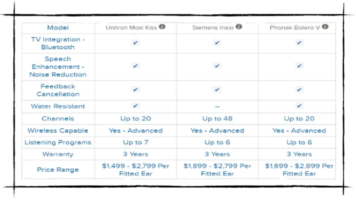
Figure 2: Existing Applications: Hearing Aid
Figure 2 shows the existing applications for hearing aids and their available features like TV Integration - Bluetooth, Speech Enhancement-Noise reduction, Feedback cancellation, Water resistant, Number of channels, Wireless capable, Listening programs, warranty and price Range. Each has a price range from $ 1,499 to $ 2,899.
Existing Approaches: Music Recognition [7]
Shazam [7] - With unlimited tagging and loads of features, the original music ID app is still the best. Shazam identifies songs quickly and accurately, and the app is fully integrated with Facebook, Twitter, Spotify, and Pandora. It has also scrapped most of the limitations they used to have on the software, meaning you can now tag as many songs as you want.
SoundHound[7]: Have a song stuck in your head, but can’t think of the name? Soundhound can help you with those songs that are on the tip of your tongue, or ear rather. This app can identify a song for you, just by humming the melody or singing a few lyrics, in addition to providing Sham-style tagging. You have to be pretty accurate with your humming for it to guess the song, because it can’t read minds (yet). Tagging a song as its playing lets you see the lyrics as they’re sung, just like karaoke. You can also check out what’s hot to see what other people are tagging.
MusiXmatch [7]: MusiXmatch has powerful lyric recognition and a large catalog of lyrics to accurately find what you’re looking for, based on song lyrics. You can tag and save lyrics, share them, and even browse lyrics while offline. The app is compatible with many third-party music players to give you lyrics as you’re listening.
CHAPTER 3 PROPOSED FRAMEWORK
3.1 Overview
Machine Learning requires building models on the data, which takes lots of computation power. Machine Learning on smart phones is typically not feasible due to the heavy loaded computation required for processing large-scale data. And the conventional Machine Learning systems do not naturally or efficiently support some very important features of large-scale streaming data. After analyzing the problems and objectives, we came up with a set of features and framework in our application. Our framework goal is to achieve an engine which aims for a lightweight Machine Learning engine with collaboration between server and cloud environment. We are testing and building models on the server and these models are saved in cloud environment which are later downloaded on smart phones for recognition.
We have reduced space complexity by reducing the number of data points used for building models. We have achieved this by clustering the data through a self-organized map. By which we have achieved less build time and space complexity of the server.
Another objective is to increase the model accuracy, using real time data. Rather than using static data we are using real time data for testing and training models. Despite of finding audio samples from open source we tried collecting audio samples from the client(smartphones) and made use of it as the models built with static data doesn't give accurate result when compared with models build with real time data.
Rather than building models for complete data we have built models in different contexts like household, emergency, office, traffic, animals and nature which shows great improved accuracy on smartphones when compared to models built by using the complete data(no context). Our application
keeps track of user information like Geo location and time and this is used to fetch that particular context and is downloaded from cloud and used.
The User can apply dynamic filters on dynamic data coming from receiver i.e., mike of a smartphone. The three types of filters used are hi-pass, low-pass, and band-pass. Our application achieves noise reduction on dynamic data by applying low-pass filter at frequency 1012 Hz. Another small feature is voice changer where you can record a sound and change pitch, tempo of the recorded sound to produce a new sound.
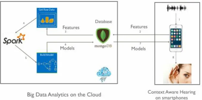
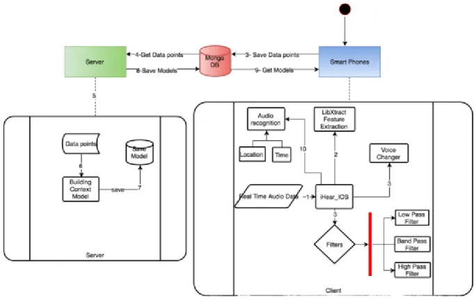
3.2 Collaboration: Cloud and Smartphone
Our proposed framework is achieved by collaboration between cloud and
smartphones. Figure 3 shows the overall flow between Smartphones and Cloud and Server. Real time data from the client is used as testing and training the classification models on the server. The Server then saves the model to Cloud, which are later downloaded on smartphones for audio recognition. In the first step, as real time audio data are collected through the receiver of smartphones, the audio features are extracted from each audio data. These features are then saved on a cloud with class name like ‘dog’, ‘door bell’ etc. On server these class names are used to distinguish data. In step two, Audio features are then saved to cloud i.e. MongoDB. There features are collected on the server in step three. When the data collection is done for a particular context (for example, if we are building a model for House hold context, we collect door bell, dog, Vacuum and Baby cry feature data from MongoDB). In step 5, as the data collection part is completed, this data is sent to Apache spark for building model for all contexts. These models are saved on MongoDB in step 6. Late in step 7 and 8, based on user location and time, Smartphones download respective model from MongoDB for audio recognition process.
Figure 3: Collaboration: Cloud and Smartphones
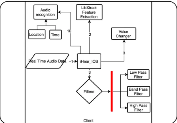
3.3 Architecture
Our proposed architecture in figure 4 includes three major parts- a) Client b) Cloud and c) Server.
a) Client: Client side process has two modules, First module is for collecting data on client for model building. In the second module audio data is collected for audio recognition. In First Module, as soon as the audio data is received through the receiver of smartphone in step 1, data send to LIbXtract library for feature extraction in step 2. We are extracting 11 features from the library, namely Mean, Standard Deviation, Variance, Spectral Centroid, Skewness, Kurtosis, ZCR, irregularity_J, irregularity_K, Rolloff, ZCR, we also normalizing the feature set to fall in a range from [11-13] each. For testing models feature data is appended to the respective context class i.e. door bell, dog bark, etc. As soon as the feature data is normalized it is saved to MongoDB in step 4.
In Second Module step 1, 2 and 3 are common. At step 9 based on user location and time,the application decides user context as an office or House or traffic and downloads respective context model from MongoDB, which are used for audio recognition at step 10. We have five different set of audio context. Each context has four classes. For example, in Office context, it has four classes, namely Door knock, phone call, Fax machine, Printer.
b) Cloud: We are using MongoDB as our cloud environment, it acts as a mediator between Client and Server. Further data are saved to the cloud by the client, this feature data is collected on the server. Later models are saved on cloud, which are downloaded on client for audio recognition.
C) Server: Machine Learning is completely done on server side. While Building models for each context - Household, traffic, nature, animal and emergency, we collect data from MongoDB as training data for Spark at step 5. For example, if we are building a model for Traffic context. We collect data for Door knock, Fax machine, Printer and phone ring from MongoDB (We can identity context data on MongoDB with the prefix name appended to feature data). This complete training data for traffic context is passed through SOM (self-organized map) in step 6 for getting clustered featured data points. Which are passed to Spark MLlib for building a traffic model. This traffic model is then saved on MongoDB for future use. This whole process is repeated for building models for all contexts and saving it in MongoDB.
Figure4: Architecture
3.4 Phase I: Feature Extraction and Selection (Smartphones)
LibXtract library is used for feature extraction and Feature Selection is done recursively . 3.4.1 Workflow:
In the feature extraction and selection workflow, as real time audio data are collected on iHear application, it is sent to LibXtract for feature extraction. These features are then passed to two approaches ‘Removing features with Low variance’ and ‘Recursive Feature Elimination’ for getting set of features which are more accurate than using all features together. The two approaches leads to this set of features - Mean, Standard Deviation, Variance, Spectral Centroid, Skewness, Kurtosis, ZCR, irregularity_J, irregularity_K, Rolloff, ZCR.
Figure 5: Workflow - Feature Extraction
3.4.2 Feature Extraction: Time Domain Features
Different types of features can be extracted from an audio signal. Here we will discuss more about Time domain features, which are dependent on time and amplitude.
Pitch: Pitch is a measure of the asymmetry of the probability distribution of a real-valued random variable about its mean. Pitch is a term used to describe how high or low a note a being played by a musical instrument or song seems to be. The pitch of a note depends on the frequency of the source of the sound. Frequency is measured in Hertz (Hz), with one vibration per second being equal to one hertz (1 Hz) [10].
A high frequency produces a high pitched note and a low frequency produces a low pitched note. Figure 5 shows how lower pitch and higher pitch looks.
Figure 6: Pitch
Loudness: The amplitude of a sound wave determines its loudness or volume. A larger amplitude means a louder sound, and a smaller amplitude means a softer sound. In Figure 6 right sound is louder than left sound. The vibration of a source sets the amplitude of a wave. It transmits energy into the medium through its vibration. More energetic vibration corresponds to larger amplitude. The molecules move back and forth more vigorously.
The loudness of a sound is also determined by the sensitivity of the ear. The human ear is more sensitive to some frequencies than to others. The volume we receive thus depends on both the amplitude of a sound wave and whether its frequency lies in a region where the ear is more or less sensitive [10].
Bandwidth: Bandwidth is the difference between the upper and lower frequencies in a continuous set of frequencies. It is typically measured in hertz, and may sometimes refer to passband bandwidth, sometimes to baseband bandwidth, depending on context. Passband bandwidth is the difference between the upper and lower cutoff frequencies of, for example, a band-pass filter, a communication channel, or a signal spectrum. In the case of a low-pass filter or baseband signal, the bandwidth is equal to its upper cutoff frequency[10].
Figure8: Bandwidth
Zero Crossing: Zero Crossing is the rate of sign-changes along a signal or the number of times that the sound signal crosses the x-axis. Zero-crossing is a point where the sign of a mathematical function change (e.g. from positive to negative), represented by a crossing of the axis (zero value) in the graph of the function. It is a commonly used term in electronics, mathematics, sound, and image processing. In alternating current, the zero-crossing is the instantaneous point at which there is no voltage present. In a sine wave or other simple waveform, this normally occurs twice during each cycle [10].
Figure 9: Zero Crossing Rate
Short Time Energy: A measure for the energy of the frames of a sound signal. This measure gives insight into the intensity and the variations in intensity of a sound signal. The amplitude of the speech signal varies appreciably with time. In particular, the amplitude of unvoiced segment is generally much lower than the amplitude of voice segments. S.T energy provides a convenient representation that reflects these amplitude variations [10].
Where s(m) is a short time speech segment obtained by passing the speech signal x(n) through window w(n):
3.4.3 Feature Extraction: Frequency Domain Features
Skewness: In probability theory and statistics, skewness is a measure of the asymmetry of the probability distribution of a real-valued random variable about its mean. The skewness value can be positive or negative, or even undefined. The qualitative interpretation of the skew is complicated. For a unimodal distribution, negative skew indicates that the tail on the left side of the probability density function is longer or faster than the right side – it does not distinguish these shapes. Conversely, positive skew indicates that the tail on the right side is longer or fatter than the left side. In cases where one tail is long but the other tail is fat, skewness does not obey a simple rule. From figure 10, we can say that wave form which are longer on the left are said to be Positive Skewness and wave forms which are longer on the right side are said to be Negative Skewness[10].
Figure11: Skewness
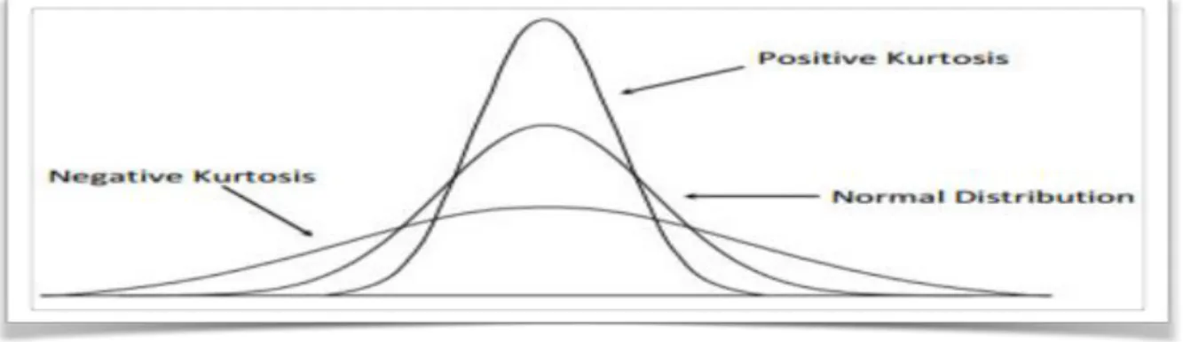
Kurtosis: is the measure of the peak of a distribution, and indicates how high the distribution is around the mean. In probability theory and statistics, kurtosis is a measure of the "tailedness" of the probability distribution of a real-valued random variable. In a similar way to the concept of skewness, kurtosis is a descriptor of the shape of a probability distribution and, just as for skewness, there are different ways of quantifying it for a theoretical distribution and the corresponding ways of estimating it from a sample
from a population. Depending on the particular measure of kurtosis that is used, there are various interpretations of kurtosis, and of how particular measures should be interpreted [10].
From figure 11, we can say that wave forms with less amplitude are said to be Negative Kurtosis and wave from with high amplitude are said to be Positive Kurtosis.
Figure 12: Kurtosis
Spectral Centroid: The spectral centroid is a measure used in digital signal processing to characterize a spectrum. It indicates where the "center of mass" of the spectrum is. Perceptually, it has a robust connection with the impression of "brightness" of a sound.
It is calculated as the weighted mean of the frequencies present in the signal, determined using a Fourier transform, with their magnitudes as the weights:
where x(n) represents the weighted frequency value, or magnitude, of bin number n, and f(n) represents the center frequency of that bin.
Figure13: Spectral Centroid
Spectral Irregularity: Spectral irregularity represents jaggedness of spectral envelope. Following figure
13, illustrate how Spectral irregularity looks like when it is represented in spectral envelope.
Figure14: Spectral Irregularity
Spectral Rolloff Point: spectral roll-off point is the frequency below which 95th percentile of the
power in the spectrum resides [30]. This is a measure of the "skewness" of the spectral shape - the value is higher for right-skewed distributions [30]. SR can tells voiced speech from unvoiced speech as unvoiced speech has a high proportion of energy contained in the high-frequency range of the
spectrum, while most of the energy for unvoiced speech and music is contained in lower bands of spectrum. Figure 14 shows the energy spectrum (cumulative energy) along frequency with 95% spectral roll-off frequency [8]. The spectral roll-off value for a frame is computed as follows:
E[f] is the energy of the signal at the frequency f. fMAX is the maximal frequency in the spectrum.
Figure15: Spectral Rolloff
Spectral Centroid: the “balancing point” of the spectral power distribution. Many types of music
involve percussive sounds which push the spectral mean higher by including high-frequency noise [30]. The spectral centroid for a frame is computed as follows:
Where: k is an index corresponding to a frequency, or small band of frequencies within the overall measured spectrum, and X[k] is the power of the signal at the corresponding frequency band. Table 3.5 shows the twelve statistics of SC in our work.
Spectrogram: A spectrogram is a visual representation of the spectrum of frequencies in a sound or other signal as they vary with time or some other variable. Spectrograms are sometimes called spectral waterfalls, voiceprints, or voice grams.
Spectrograms can be used to identify spoken words phonetically, and to analyze the various calls of animals. They are used extensively in the development of the fields of music, sonar, radar, and speech processing, seismology [1].
The instrument that generates a spectrogram is called a spectrograph.
Figure16: Spectrogram
Mel Frequency Cepstral Coefficients (MFCCs): MFCCs is the feature popularly used for speech
recognition and audio classification due to its effectiveness in representing the spectral variations of audio. The MFCCs stands in the shape of the spectrum with few coefficients. The cepstrum is the Fourier Transform (or Discrete Cosine Transform DCT) of the logarithm of the spectrum. Instead of the Fourier spectrum, the Mel-cepstrum is the cepstrum computed on the Mel-bands. By using of the mel scale, the mid-frequency part of the signal is taken better taken into account. The MFCCs are the coefficients of the Mel cepstrum.
MFCCs are commonly derived as follows: This is shown in figure 16. 1. Take the Fourier Transform of (a windowed excerpt of) a signal.
2. Map the log amplitudes of the spectrum obtained above onto the mel scale, using triangular overlapping windows.
3. Take the Discrete Cosine Transform of the list of mel log-amplitudes, as if it was a signal.
4. The MFCCs are the amplitudes of the resulting spectrum
Figure17: MFCC 3.4.4 Feature Selection[13]:
In Machine Learning and statistics, feature selection, also known as variable selection, attribute selection or variable subset selection, is the process of selecting a subset of relevant features (variables, predictors) for use in model construction. Feature selection techniques are used for three reasons: • Simplification of models to make them easier to interpret by researchers/users.
• shorter training times,
• enhanced generalization by reducing overfitting
We are doing a feature selection by following two approaches: Removing Features with Low Variance:
Variance Threshold is a simple baseline approach to feature selection. It removes all features whose variance don’t meet some threshold. By default, it removes all zero-variance features, i.e. features that have the same value in all samples.
As an example, suppose that we have a dataset with Boolean features, and we want to remove all features that are either one or zero (on or off) in more than 80% of the samples. Boolean features are Bernoulli random variables, and the variance of such variables is given by
so we can select using the threshold .8 * (1 - .8). Recursive Feature Elimination:
Given an external estimator that assigns weights to features (e.g., the coefficients of a linear model), recursive feature elimination (RFE) is to select features by recursively considering smaller and smaller sets of features. First, the estimator is trained on the initial set of features and weights are assigned to each one of them. Then, features whose absolute weights are the smallest are pruned from the current set features. That procedure is recursively repeated in the pruned set until the desired number of features to select is eventually reached.
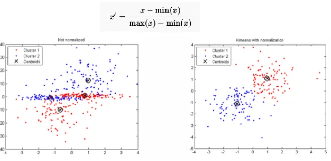
3.4.5 Feature scaling & Data Normalization:
The result of standardization (or Z-score normalization) is that the features will be rescaled so that they’ll have the properties of a standard normal distribution with μ=0 and σ=1, where μ is the mean (average) and σ is the standard deviation from the mean; standard scores (also called z scores) of the samples are calculated as follows:
Feature scaling was used to standardize the range of independent variables or features of data. The simplest method is rescaling the range of features to scale the range in [0, 1] or [−1, 1].
Figure18: Feature Scaling
Figure 18 shows the difference between k-means normalized data vs without normalized data. K-means cluster after normalizing the data look more organized data points on the clusters.
Figure19: Normalized Real time data
Data normalization is computational data transformations intended to remove certain systematic biases from audio data. In figure 19, We have normalized real time feature data to normalized feature data with a range of [10-12] by applying some mathematical formula.
3.5 PHASE II: MODEL BUILDING for BIG DATA ANALYTICS ON CLOUD Following are the steps involved in Phase II.
Phase II-I: Audio Class Signature Generation using Machine Learning Algorithm
Phase II-II: Audio Classification using Supervised Machine Learning Algorithms based on Audio Signature 3.5.1 Phase II: Model Building Workflow:
Machine Learning completely is done on the server side. While building models for a particular context, server gets all the data required for a particular context as a training set for building models. These data are sent to SOM (self-organized map) to get clustered data points. These clustered data points are sent to Spark MLlib for model building. Here we are building decision tree and random forest. These are saved to MongoDB for further use.
3.5.2 Phase II - I: Audio Signature Generation
Audio signature is generated for each audio class of a context using Self Organizing Maps (SOM). SOM is a type of artificial neural network (ANN) - Trained using unsupervised learning to produce a low-dimensional signature for given audio features. Discretized representation of the input space of the training samples, called a map.
From figure 21, consider House hold context, which has 5 classes, namely vacuum, Baby cry, dog bark, door knock, phone ring. Each class has its own feature data which is send to Self-organized map for clustered data. Feature data of the same type are clustered to one group. Resultant clusters data occupy less space.
3.5.3 Phase II - II: Audio Classification[9]
In Machine Learning and statistics, classification is the problem of identifying to which of a set of categories (sub-populations) a new observation belongs, on the basis of a training set of data containing observations (or instances) whose category membership is known. An example would be assigned a given email into "spam" or "non-spam" classes or assigning a diagnosis to a given patient as described by observed characteristics of the patient (gender, blood pressure, presence or absence of certain symptoms, etc.). Classification is an example of pattern recognition[13][9].
a. Naive Bayes:
The Naive Bayes technique is used to design the classifiers using the features and labels of the datasets. In general the Machine Learning algorithms must be trained in order to classify and predict. The Naive Bayes algorithm is one of the classification algorithm based on Bayes theorem to train the dataset. It generates the models to identify the relation between input data and the predictable data. These classifiers consider each attribute as independent and generates the features and using each feature it generate the probability of identifying.
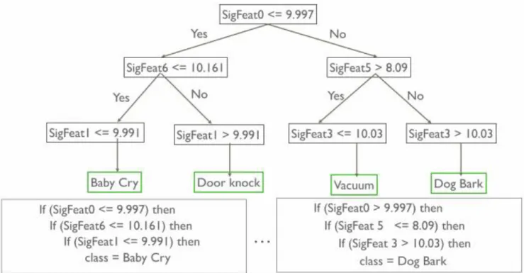
b. Decision Tree:
A decision tree is a decision support tool that uses a treelike graph or model of decisions and their possible consequences, including chance event outcomes, resource costs, and utility. It is one way to display an algorithm. Decision trees are commonly used in operations research, specifically in decision analysis, to help identify a strategy most likely to reach a goal, but are also a popular tool in Machine Learning.
A decision tree is a flowchart-like structure in which each internal node represents a "test" on an attribute (e.g., whether a coin flip comes up heads or tails), each branch represents the outcome of the test and each leaf node represents a class label
Decision Tree is a supervise Machine Learning algorithm. It builds audio classifiers using audio signatures. Classification rules extracted from the decision tree classifiers are saved and reused for client side audio recognition.
Figure 22 shows how decision tree flow looks, and how it parses through the branches to reach the final results based on intermediate nodes that is SigFeat features. For example, for recognizing ‘baby cry’ sound it goes to 3 levels, in level one the root node checks if SigFeat0 is less than or equal to 9.997 if it is true, then it goes to next level node to check if SigFeat6 is less than or equal to 10.161. If this is true, then it goes to level three nodes and checks if SigFear1 is less or equal to 9.991. If this condition is true, it comes to conclusion that the sound is a ‘Baby cry’.
3.6 PHASE III: CONTEXT AWARE AUDIO RECOGNITION (SMARTPHONES):
Figure23: Context Aware Models
Context aware systems are a component of ubiquitous computing or pervasive computing environments. CAAR makes the mobile platforms capable:
1. Sensing the users and their current state, exploiting context information to significantly reduce demands on human attention.
2. Minimizing noises and maximizing the recognition accuracy with context-awareness.
3. Scalable and efficient recognition with a minimum set of models for the lightweight Machine Learning engine.
Figure 23 shows, how we have divided our context aware model considering the user location and time.
In
our application, we have modeled five important contexts based on the geographical prevalence and time domain of the user. Following are the five contexts we have considered:Home Context:
This context has all basic household sounds a user can have. This context is chosen when the user is in their house.In our application, we have considered only four sounds of households. Following are the four classes/sounds we considered:
1. Door knock. 2. Vacuum cleaner. 3. Dog bark. 4. Baby cry.
Nature Context:
This context consists of all basic nature sounds. This context is chosen when the user is in their outdoor near beach or forest. In our application, we have considered only four sounds of Nature. Following are the four classes/sounds we considered:
1. Ocean waves. 2. Fire.
3. Rain. 4. Thunder.
Office Context:
This context consists of all basic Office sounds. This context is chosen when the user is in their office. In our application, we have considered only four sounds of office. Following are the four classes/sounds we considered:
1. Fax machines. 2. Phone rings.
3. Printer. 4. Door Knock.
Traffic Context:
This context has all basic traffic sounds we have. This context is applied when the user is moving in traffic. In our application, we have considered only four sounds of traffic. Following are the four classes/sounds we considered: 1. Car horn. 2. Bike exhaust. 3. Train. 4. Helicopter. Emergency Context:
This context has all basic emergency sounds we have. This context is applied all the time, regardless of user location. In our application, we have considered only four sounds of emergency. Following are the four classes/sounds we considered:
1. Police siren. 2. Ambulance. 3. Fire alarm. 4. Scream.
CHAPTER 4
IMPLEMENTATION AND EXPERIMENT SETUP
4.1 ImplementationFor implementation, we have used following
•Python, Scala: Python and Scala are used as programming languages to use Apache Spark MLlib and Self organized map.
•Apache Spark 1.5.2: Apache Spark is used for audio streaming and classification algorithms. •Mongo DB: Mongo DB is used for storing feature data and user basic information. It acts like
a mediator between server and client,
4.2 Experiment Setup
We have conducted and evaluated my experiments on three different machines. We have used machine 1 and machine 2 for Machine Learning i.e., training and testing models. Machine 3 is used for iHear application.
Machine 1:
•Ubuntu 14.04 – we have used Ubuntu 14.04 version. We have used OS X mac platform for building models.
•Memory: 15.6 GB – with 15.6 GB RAM size.
•Processor: Intel® Xeon(R) CPU E3-1230 V2 @ 3.30GHz × 8 Machine 2:
•OS X – we have used OS X mac platform for building models. •Memory: 8 GB - with 8 GB RAM size.
•Processor: 2.2 GHz Intel Core i7 Machine 3:
CHAPTER
5
EVALUATIONS
5.I Evaluation Plan
Following is the evaluation plan, we will go through step by step to justify our proposed solutions:
1. Noise Reduction:
In this evaluation we will justify how the noise reduction process works with iHear filters. We performed tests with noise data in this case, it’s Vacuum sound. This noise sound is combined with a song, and we will see the resultant sound with reduced noise sound.
2. Feature Extraction:
In feature extraction phase, we will show how audio features look when the audio is captured dynamically from the client.
3. Feature Selection: Accuracy:
Feature selection techniques are used for two main reasons: simplification of models to make them easier to interpret by researchers/users, shorter training times. We will evaluate this section by taking a different feature set and evaluate which feature set is more accurate.
4. Feature Scaling and Normalization: Accuracy:
In this section we will evaluate with normal feature set and normalized feature set, and observe the accuracy for both of them in terms of building models.
5. Audio Classification:
In audio classification, we are evaluating our light weight engine with Context aware models and Signature to other regular approaches to see which one gives better results in build time, accuracy and space. Following is the evaluation for audio classifications.
1. context-aware audio classification:
Based on user location and time, we have differentiated five contexts namely office, house, traffic, nature and animals. For building models for each of the contexts, we have two approaches:
(A) Dynamic Learning/Dynamic Recognition:
In Dynamic Learning/Dynamic Recognition, for training the models we collected real time(Dynamic) data from smartphones and for testing the models we use same Dynamic data collected from smartphones for getting accuracy.
(B) Static Learning/ Dynamic Recognition:
In Static Learning/Dynamic Recognition, for training the models we collected static data which are audio smokes collected from the internet and for testing the models we used real time audio data (Dynamic data) collected from smartphones for getting accuracy.
2. without context audio classification:
Another approach is without using any context, we will evaluate all models together as one here. We have two approaches in building models:
(A) Dynamic Learning/Dynamic Recognition:
In Dynamic Learning/Dynamic Recognition, for training the models we collected real time (Dynamic) data from smartphones and for testing the models we use same Dynamic data collected from smartphones for getting accuracy.
(B) Static Learning/ Dynamic Recognition:
In Static Learning/Dynamic Recognition, for training the models we collected static data which are audio smokes collected from the internet and for testing the models we used real time audio data (Dynamic data) collected from smartphones for getting accuracy.
5.2 Noise Reduction
Figure 24, is the representation of a song data with time domain on x-axis and frequency on Y- axis. As we can see song data is ranging from {-0.2, 0.1}.
Figure 24: Song data
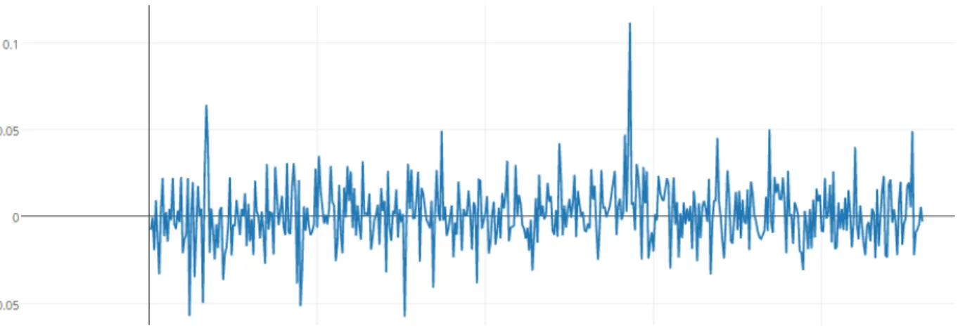
Figure 25, is the representation of noise data (vacuum sound) with time domain on x-axis and frequency on the Y- axis. From the wave form, we can observe that vacuum sound is ranging from {-0.05, 0.05}.
Figure26, represents noise data (vacuum sound) and song data together, with time domain on x-axis and frequency on the Y- axis. Form the below waveform, we can observe that Sound data with noise data is ranging from {-0.05, 0.1}
Figure 26: Sound + Vacuum data
Now by applying iHear dynamic Low pass filter at 1400 Hz frequency, we can reduce the noise data(Vacuum) by 60-70%. This can be shown in Figure27, where vacuum data ranged from {-0.05, 0.05} is neglected. Resulted sound ranged from {-0.02, 0.02}.
5.3 Phase I - I: Feature Extraction
The Following figures show how each feature looks when plotted on a graph. This graph is the representation of the dynamic audio wave.
Mean:
Mean graph is plotted for three different sounds namely Door bell, police siren and vacuum. With Mean values on Y axis and time(milliseconds) on x axis.
Figure 28: Feature -Mean
Variance: Variance graph is plotted for their sounds namely Door bell, police siren and Vacuum. With Mean values on Y axis and time (milliseconds) on x axis.
Spectral Centroid: Spectral centroid graph is plotted for their sounds namely Door bell, police siren and Vacuum. Spectral centroid values on Y axis and time (milliseconds) on x axis.
Figure 30: Feature - Spectral Centroid
Skewness: Skewness graph is plotted for their sounds namely Door bell, police siren and Vacuum. With Skewness values on Y axis and time (milliseconds) on x axis.
ZCR: ZCR graph is plotted for their sounds namely Door bell, police siren and Vacuum. With ZCR values on Y axis and time (milliseconds) on x axis.
Figure 32: Feature - ZCR
Kurtosis: Kurtosis graph is plotted for their sounds namely Door bell, police siren and Vacuum. With Kurtosis values on Y axis and time (milliseconds) on x axis.
Irregularity: Irregularity graph is plotted for their sounds namely Door bell, police siren and Vacuum. With Irregularity values on Y axis and time (milliseconds) on x axis.
Figure 34: Feature - Irregularity
MFCC: MFCC graph is plotted for their sounds namely Door bell, police siren and Vacuum. With MFCC values on Y axis and time (milliseconds) on x axis.
5.4 Phase I - II: Feature Selection: Test Cases
In this evaluation we will find the best set of features for best accuracy. Following is the table with different test cases with different set of features. Test 1 has 27 features, test 2 has 16 features, test 3 has 12 features and test 4 has 9 features. In the next sections we will we discuss about accuracy for each test case chosen, and find the best fit.
Test 1 27 Mean, Standard Deviation, Variance, Skewness, Kurtosis, Spectral
Mean, Spectral Variance, Spectral Standard Deviation, Spectral Skewness, Spectral Kurtosis, Spectral Centroid, MFCC, Irregularity_k, Irregularity_j, Tristimulus_1, Tristimulus_2, Tristimulus_3, Smoothness, Spread, ZCR, Rolloff, Loudness,
Flatness, Tonality, Breast, Lowest_Value, Highest Value
Test 2 16 Mean, Standard Deviation, Variance, Spectral centroid, Spectral
Skewness, ZCR, MFCC, Loudness, kurtosis , irregularity_k, irregularity_j, Tristimulus_2, skewness, highest_value, Rolloff,
Tonality
Test 3 12 Mean, Standard Deviation, Variance, Spectral centroid, ZCR,
Loudness, kurtosis , irregularity_k, irregularity_j, skewness, highest_value, MFCC
Test 4 9 Mean, Variance, Spectral centroid, Loudness, kurtosis ,
irregularity_j, skewness, highest_value, MFCC
5.4.1 Feature Selection: Accuracy
Figure 36, shows the accuracy for all four test cases choose in the feature selection evaluation process. From the results, we can see that test 3 with a feature set [Mean, Standard Deviation, Variance, Spectral centroid, ZCR, Loudness, kurtosis, irregularity_k, irregularity_j, skewness, highest_value, MFCC] has high accuracy 89% than remaining three test cases. Test case 1 has an accuracy of 52% for decision tree and 51% of random forest, test case 2 has an accuracy of 68% for decision tree and 70%
of random forest, test case 4 has an accuracy of 74% for decision tree and 69% of random forest. Which are less than test case 2 accuracy. Our engine chooses test case 3 feature set as for building models.
Figure 36: Feature Selection - accuracy
5.5 Phase 1-3: Data Normalization - Accuracy
Figure 37: Data Normalization - accuracy
0
25
50
75
100
Test 1 Test 2 Test 3 Test 4
Accu
racy
Decision Tree Random Forest
0
23
45
68
90
Original Features
Normalized
Features
Figure 37, shows the accuracy of models for both original features and normalized features. With original feature data set, each features is ranged from 0 to 49999. In normalized feature data set each feature is ranged from 11 to 14.
5.6 Phase II-III: Audio Classification Evaluation
In this audio classification evaluation. We are considering two level hierarchy. The First level is done on the client, we have Learned with static data and learning with dynamic data. Each of these learnings has two approaches Feature Approach and Signature Based Approach. Each of these approaches has two process - ’Audio recognition with contexts’ (AR) and ‘Context Aware audio recognition’(CAAR). This complete hierarchy is showed in figure 38.
5.7Context Aware Audio Classification
5.7.1 Context Aware Audio Classification: Dynamic Learning/ Dynamic Recognition Context Aware Audio Classification: Household
In figure 39, we are evaluating Household context model accuracy with all feature data set and clusters featured data set ranging from 650 to 100. For example, as house hold context has four classes - Door knock, baby cry, vacuum sound, Dog bark. Each having a feature data count of 1250. So total feature count of the Household context is 1250 * 4 = 6000 data points. Signature (cluster: 650) means data points for each class are clustered in 650 from 1250 original features. NowSignature (cluster: 650) has total data set of = 650 * 4 = 2600 data points. Signature (cluster: 400) means data points for each class are clustered to 400 from 1250 original features. NowSignature (cluster: 400) has total data set of = 400 * 4 = 1600 data points. Signature (cluster: 200) means data points for each class are clustered in to 2000 from 1250 original features. NowSignature (cluster: 200) has total data set of = 200 * 4 = 800 data points. Signature (cluster: 100) means data points for each class are clustered in to 100 from 1250 original features. NowSignature (cluster: 100) has a data set as = 100 * 4 = 400 data points.
From figure 39, We can observe that house hold context model with total feature has an accuracy of 82% for decision tree and 81 % for random forest. Whereas Signature (cluster: 650) features has an accuracy of 80% for decision tree and 78 % for random forest.Signature (cluster: 400) features has an accuracy of 80% for decision tree and 79 % for random forest. Signature (cluster: 200) features has an accuracy of 82% for decision tree and 74 % for random forest. Signature (cluster: 100) features has an accuracy of 73% for decision tree and 63 % for random forest.
From this evaluation we can say that, Signature(cluster: 200) has the same accuracy as that of total features. From figure 40, Signature(cluster: 200) has a build time of 53 sec and data points count as 800 where as Total feature has a build time of 70 sec and data points count as 6000. So by using
signature approach we have reduced reduced the build time from 70 sec to 53 sec and data points count from 6000 to 800 which is 84% size drop.
Context Aware Audio Classification: Nature
In figure 41, we are evaluating Nature context model accuracy with all feature data seta and clusters featured data set ranging from 650 to 100. From figure 41, we can observe that nature context model with total feature has accuracy of 81% for decision tree and 79% for random forest. Whereas Signature (cluster: 650) features has an accuracy of 81% for decision tree and 74% for random forest. Signature (cluster: 400) features has an accuracy of 80% for decision tree and 79% for random forest. Signature (cluster: 200) features has an accuracy of 76% for decision tree and 74% for random forest. Signature (cluster: 100) features has an accuracy of 76% for decision tree and 73% for random forest.
Form the figure 42, we can observe that total feature data set took build time as 45 sec and data points count as 5000. Signature (Cluster: 650) took build time as 55 sec and data points count as 2800. Signature (Cluster: 400) took build time as 50 sec and data points count as 1800. Signature (Cluster: 200) took build time as 35 sec and data points count as 800.Signature (Cluster: 100) took build time as 25 sec and data points count as 400.
Form this evaluation we have two observations, if we want less build time and less data points, we can choose Signature(Cluster: 200) or Signature(Cluster: 100) approach as both has less build time and less data size(20% of original feature data count). If we consider accuracy we can go for Signature (Cluster: 650) as it has same accuracy 81% compared with total feature data accuracy. It’s a tradeoff between accuracy, time/size in this scenario.
Figure 41: Context Aware Audio Classification Nature- Accuracy
Context Aware Audio Classification: Emergency
In figure 43, we are evaluating Emergency context model accuracy with all feature data seta and clusters featured data set ranging from 650 to 100. From figure 43, we can observe that Emergency context model with total feature has an accuracy of 90% for decision tree and 87% for random forest. Whereas Signature (cluster: 650) features has an accuracy of 90% for decision tree and 88% for random forest. Signature (cluster: 400) features has an accuracy of 91% for decision tree and 89% for random forest. Signature (cluster: 200) features has an accuracy of 90% for decision tree and 89% for random forest. Signature (cluster: 100) features has an accuracy of 84% for decision tree and 81% for random forest.
From figure 44, we can observe that total feature data set took build time as 50 sec and data points count as 6000. Signature (Cluster: 650) took build time as 55 sec and data points count as 2200. Signature (Cluster: 400) took build time as 48 sec and data points count as 1500. Signature (Cluster: 200) took build time as 34 sec and data points count as 800. Signature (Cluster: 100) took build time as 25 sec and data points count as 400.
From this evaluation we can say that, Signature (cluster: 400) has more accuracy that of total features accuracy. Even build time has reduce from 50 sec to 48 sec, and data point count has reduce from 6000 to 1500 (25% of total size).
Figure 43: Context Aware Audio Classification Emergency- Accuracy