A Thesis Submitted to the Faculty
of
Drexel University by
Tingshan Huang in partial fulfillment of the requirements for the degree
of
Doctor of Philosophy December 2015
Dedications
Acknowledgments
I would like to express my deepest gratitude to my advisors, Drs. Nagarajan Kandasamy and Harish Sethu, for their continuous inspiration, support and guidance in the last 65 months. I am grateful to Drs. Kandasamy and Sethu for introducing me into the field of anomaly detection at the first place and for their constant encouragement in my work and career. I appreciate their time and effort in delivering knowledge, insight, guidance and suggestions that made this dissertation pos-sible. I am fortunate to have two co-advisors who are outstandingly knowledgeable and inspiring. What I have learned from them has not only reshaped my way of thinking, but also my attitude toward life.
Many thanks are due to the members of my committee, Drs. Nagarajan Kandasamy, Spiros Mancoridis, James Shackleford, Steven Weber and Harish Sethu. I would like to thank them all for agreeing to spend their precious time to serve on my committee and for providing valuable feedback that allows me to improve my work. I would also like to express my gratitude to Drs. Matthew Stamm and John Walsh for their helpful suggestions on my work.
I am also thankful to my friends and colleagues at Drexel University, especially Xiaoyu Chu, Rui Wang, Yao Yu, Bradford Boyle, Raymond Canzanese, Guyue Han, Salvador DeCelles and Ni An, for their invaluable help and friendship. I am grateful for the assistance provided by ECE staffover the years, especially those from Chad Morris, Kathy Bryant, Tanita Chapelle, Phyllis D. Watson and Sean Clark.
Finally, I owe a debt of gratitude to my family, especially my fianc´e Shuyang Chen, for their continuous understanding, encouragement, and love.
Table of Contents
LIST OF TABLES . . . viii
LIST OF FIGURES . . . ix
ABSTRACT . . . xiii
1. Introduction . . . 1
1.1 Resource-efficient system monitoring . . . 3
1.1.1 Monitoring with known correlation . . . 5
1.1.2 Monitoring with unknown correlation . . . 6
1.2 Resource-efficient system monitoring using compression and compressive sampling . 7 1.2.1 Resource-efficient system monitoring using compression . . . 7
1.2.2 Resource-efficient system monitoring using compressive sampling . . . 9
1.2.3 Comparing compression and compressive sampling . . . 10
1.3 Anomaly detection . . . 11
1.3.1 Signature-based techniques for anomaly detection . . . 12
1.3.2 Statistic-based techniques for anomaly detection . . . 12
1.3.3 Principal component analysis for anomaly detection. . . 14
1.4 Contribution to resource-efficient monitoring . . . 15
1.4.1 C-MON: monitoring using compression in the best basis . . . 15
1.4.2 CS-MON: monitoring using adaptive-rate compressive sampling. . . 17
1.5 Contribution to anomaly detection . . . 19
1.5.1 Anomaly detection with compressed measurements . . . 19
1.5.2 Anomaly detection with the maximum subspace distance . . . 21
2. An Efficient Strategy for Online Performance Monitoring of Datacenters via Adaptive Sampling . . . 25
2.1 Introduction . . . 25
2.2 Experimental Setting. . . 29
2.3.1 Sparse Representation of Signals. . . 32
2.3.2 The Best Basis Algorithm . . . 33
2.3.3 Compression-based Online Monitoring Method . . . 34
2.4 Compressive Sampling of System Measurements . . . 35
2.4.1 Incoherent Sampling of the Signal . . . 35
2.4.2 Recovering the Original Signal . . . 37
2.4.3 A CS-based Online Monitoring Strategy . . . 38
2.5 Adaptive-rate compressive sampling. . . 39
2.5.1 Overview of the CS-MON Strategy . . . 39
2.5.2 The Compressive Sampling Block . . . 41
2.5.3 The Cross-Validation Block . . . 42
2.5.4 The Kalman Filter block . . . 45
2.5.5 Summary of the Adaptive-Rate Model Operation . . . 46
2.6 Performance Evaluation . . . 46
2.6.1 Signal Reconstruction Quality using CS-MON . . . 47
2.6.2 Comparing the CS-MON and C-MON Strategies . . . 53
2.6.3 Case Studies . . . 56
2.7 Related Work . . . 58
2.8 Summary . . . 60
3. Anomaly detection in computer systems with compressed measurements . . . 62
3.1 Introduction . . . 62
3.2 Experimental settings . . . 65
3.3 Anomaly Detection using Compressed Samples . . . 65
3.3.1 Detection of spikes from compressed samples . . . 67
3.3.2 Detection of trends from compressed samples . . . 70
3.3.3 PCA-based detection from compressed samples . . . 73
3.4 Performance evaluation . . . 77
3.4.1 Detection of Spikes and Abrupt Changes . . . 77
3.4.3 PCA-based Detection of Spikes and Abrupt Changes. . . 79
3.5 Related work . . . 80
3.6 Summary . . . 81
4. Fast and Distributed Detection of Anomalies in Feature Matrices of Network Traffic . . . 83
4.1 Introduction . . . 83
4.1.1 Problem Statement and Contributions . . . 85
4.2 Related Work . . . 87
4.3 The Metric . . . 90
4.3.1 The subspace distance . . . 90
4.3.2 The maximum subspace distance . . . 91
4.3.3 Comparison with principal angles . . . 91
4.4 The Centralized Algorithm . . . 92
4.4.1 The rationale behind allowingkA=kB. . . 93
4.4.2 Subspace distance and the projection matrix . . . 94
4.4.3 Estimating the optimal subspace dimension . . . 98
4.4.4 Complexity analysis . . . 100
4.5 Distributed Algorithm . . . 102
4.5.1 Assumptions and system model . . . 102
4.5.2 Average consensus . . . 103
4.5.3 Distributed power iteration method . . . 104
4.5.4 ThegetESD-D algorithm . . . 106
4.5.5 Complexity Analysis . . . 107
4.6 Simulation results . . . 110
4.6.1 Verification of theorems . . . 110
4.6.2 Estimation of subspace distance . . . 110
4.6.3 Evaluating the distributed power iteration method . . . 113
4.6.4 Application on anomaly detection. . . 114
4.6.5 Anomaly detection using Projection Residual . . . 117
4.6.7 Running time comparison . . . 120
4.7 Concluding Remarks. . . 121
5. Conclusions and future work . . . 122
5.1 System monitoring . . . 122
5.1.1 C-MON . . . 122
5.1.2 CS-MON . . . 123
5.2 Anomaly detection . . . 123
5.2.1 Anomaly detection with compressed measurements . . . 124
5.2.2 Centralized anomaly detection using covariance matrices . . . 124
5.2.3 Distributed anomaly detection using raw measurements . . . 125
5.3 Future work . . . 125
List of Tables
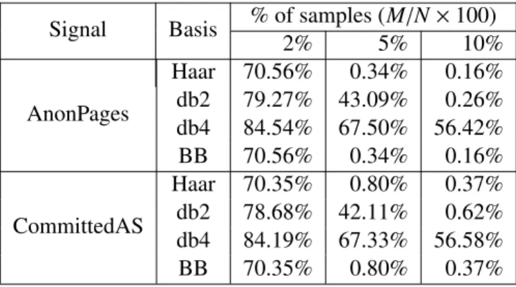
2.1 Percentage of coefficients needed to keep the relative error within 1% under each rep-resentation basis. . . 33 2.2 Average coherence between anM×Nrandom Gaussian sensing basis and the different
representation bases whenN=2048. . . 36 2.3 The average sample size used by CS-MON to reconstruct the AnonPages and
Commit-teAS signals for different sparsity levels. . . 50 2.4 Relative error between the original AnonPages and CommittedAS signals, and the
cor-responding reconstructions, achieved by C-MON. . . 52 2.5 Storage costs incurred by C-MON and CS-MON under different sparsity levels when
sampling the AnonPages signal. . . 54 2.6 The packetization delay incurred in seconds for various lengths of the measurement
window and sampling rate. . . 55 4.1 Number of principal components that captures 99.9% variance with varyingλ, when
List of Figures
1.1 The system monitoring model in the case of monitoring a data center. . . 4 1.2 Categorization of methods for system monitoring and anomaly detection. The
cate-gories to which the proposed methods of this dissertation belong are enclosed in the dotted lines.. . . 4 1.3 The system monitoring model using compression. . . 8 1.4 The form of data at different stages of the monitoring model using compression. (a) the
original data to be collected. (b) the representation of the data in the Haar wavelet basis. (c) the compressed form of the data after applying thresholding on the coefficients. (d) the reconstructed data after applying inverse wavelet transform on the compressed form of data. . . 8 1.5 The system monitoring model using compressive sampling . . . 9 1.6 The form of data at different stages of the monitoring model using compressive
sam-pling. The original data is the same as in Figure 1.4. (a) the sampled data that is also in the compressed form. (b) the reconstructed data after applying reconstruction algorithm on the compressed form of data. . . 10 1.7 Principal components of two-dimensional data. . . 14 1.8 The sparsity of data in (a) in two wavelet bases: Haar and db2. (a) An example of data
series reflecting the memory allocated to a virtual machine. (b) Representation of the data in Haar wavelet basis. (c) Representation of the data in db2 wavelet basis. The data is more concisely represented in the db2 basis. . . 16 1.9 The system monitoring model of C-MON. . . 17 1.10 Change in the sparsity level over time for the measurement of memory usage of a virtual
machine in a data center. . . 17 1.11 The system monitoring model of CS-MON. . . 18 1.12 The example of subspace distance between two sets of principal components. (a) Two
sets of principal components: {a1,a2} and {b1,b2}. (b) The subspace angle between a pair of subsets of principal components when the number of principal components included in each subset increases from 0 to 2. The subspace angle is maximum when the subspace dimension is 1. The maximum subspace angle isθ, i.e., the angle between
2.1 (a) The overall system architecture hosting the Trade6 application which implements a stock-trading service that allows users to browse, buy, and sell stocks. (b) Example of workload provided to the testbed in our experiments, plotted in granularity of 30 seconds. 30 2.2 Measurements corresponding to the AnonPages and CommittedAS signals collected
over a 48-hour operating period. . . 30 2.3 Waveforms corresponding to three members of the Daubechies wavelet family. The
Haar is the simplest wavelet that captures discontinuities in the data; db2 and db4 also show similarity with our data but have longer waveforms, leading to better frequency resolution. . . 32 2.4 Implementation of compressive sampling in our system that takesN data items over a
time period as input and returnsMsamples, whereMN. . . 38 2.5 Workflow for the adaptive-rate compressive sampling strategy. The workflow comprises
three major steps: compressive sampling, cross validation, and prediction of signal sparsity. . . 40 2.6 The timeline for the execution of each block in the adaptive-rate sampling strategy.
Here CS denotes the compressive sampling block, CV, the cross validation block, and KF, the Kalman filter. . . 40 2.7 The relative error achieved by various sample sizes, given different sparsity levels within
the AnonPages signal. Best viewed in color. . . 41 2.8 Overlay of the actual sparsity of the AnonPages signal witha posteriorivalues ˜s
ob-tained by the cross validation block. Here sparsity is defined as the number of co-efficients needed to capture 99% of the original signal. The plots show the ˜s values obtained using the following initial guesses for the sparsity levels: 4%, 17%, and 30%. . . 48 2.9 Predictions for sparsity values provided by the Kalman filter for the AnonPages
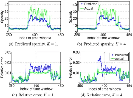
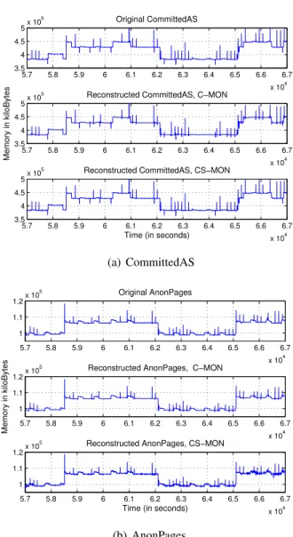
sig-nal when the filter’s state is updated: (a) during each time window, that is K = 1, and (b) once every four windows, K = 4. The relative error between the actual and reconstructed signals when the filter state is updated each window and once every four windows is shown in (c) and (d), respectively. . . 49 2.10 The original CommittedAS and AnonPages signals, and the same signals recovered by
C-MON using 5% of the coefficients in the basis found by the best basis algorithm. The signal recovered by CS-MON with 15% error tolerance is also shown for comparison purposes.. . . 51 2.11 The CPU overhead incurred by the sampling and encoding processes associated with
the C-MON and CS-MON strategies on the local machine. The signal reconstruction overhead incurred by the monitoring station is not included here. Both strategies were implemented in MATLAB and executed on an AMD Athlon II 3.0 GHz processor. . . 53
2.12 The relative error achieved by C-MON and CS-MON when using smaller measurement
windows.. . . 55
2.13 The write activity signal collected from the testbed that measures the number of disk sectors written. . . 57
2.14 Hit rate when detecting a 1.6% violation in the write activitysignal, achieved by C-MON, CS-C-MON, and random sampling. The length of the measurement window is N=64. . . 58
2.15 The slope estimated by C-MON, CS-MON and random sampling over 40 time windows for CommittedAS.. . . 59
3.1 Signals corresponding to: (a) I/O activity collected at the database tier showing the number of sectors written to disk and (b) total amount of memory allocated by processes in the system. Note that a memory leak has been injected around the 24 hour mark. . . 66
3.2 The sample variance of the compressed samples forwrite activitydata and the spike-free data in each time window. . . 69
3.3 The variance of the random samples collected forwrite activityin each time window.. . . . 70
3.4 The average value of the originalCommittedASdata in each time window overlaid with the scaled average of the compressed samples and random samples. . . 72
3.5 An overlay of the hit rate achieved as a result of using the compressed samples versus that of random sampling. . . 78
3.6 Slope estimates obtained forCommittedASusing the compressed data for different sam-ple sizes; overlay of the estimated slope values obtained using the original, compressed, and randomly sampled data. . . 79
3.7 The projection residual of the write activitysignal is shown in (a) wherein windows containing a spike have extremely large projections on the anomalous subspace. The achieved hit rate is shown in (b) when the false alarm rate is fixed as 0.5%. The length of the measurement length is set toN =64 and the sample size varies from 3% to 50%. . 80
4.1 ThegetESD algorithm: An efficient algorithm for finding an effective subspace dimen-sion (ESD) and the corresponding estimate of the maximum subspace distance between the two given matrices,ΣA andΣB. . . 101
4.2 The average consensus procedure. . . 104
4.3 The centralized power iteration procedure. . . 104
4.5 The distributed algorithm,getESD-D running at noden to find an effective subspace
dimension (ESD) and the corresponding estimate of the maximum subspace distance between the two given datasets,XandY. . . 108 4.6 The subspace angle and singular values ofP1:k,1:kwith varyingk. . . 111 4.7 The optimal and the effective subspace dimension for estimating the maximum
sub-space distance between covariance matrices corresponding to consecutive time win-dows in Internet backbone traffic traces. . . 112 4.8 Relative percentage error of the estimated maximum subspace distance between
covari-ance matrices corresponding to consecutive time windows in Internet backbone traffic traces. . . 112 4.9 Estimated principal component using distributed power iteration . . . 113 4.10 The mean square error between the actual principal component with the estimated
prin-cipal component. The estimation of prinprin-cipal component is performed using the dis-tributed power iteration and the centralized power iteration when the sample size in-creases. . . 114 4.11 The amount variance captured by each principal components of the test data model . . . 116 4.12 The amount variance captured by each principal components of the histogram data . . . 116 4.13 Projection residual of dataset BEFORE and AFTER onto normal subspace. Top: the
dimension of normal subspace is a result of our algorithm, getESD. Bottom: the dimen-sion of normal subspace is the minimum number of principal components that captures 99.5% of the variance in the dataset. . . 118 4.14 Receiver operating characteristic curve as a result of getESD and the subspace method. . . 118 4.15 Projection residual of test data in anomalous subspace, the dimension of which is
de-fined by our method and the subspace method. Top: dataset BEFORE. Bottom: dataset AFTER . . . 120 4.16 Subspace distance using different number of principal components . . . 120 4.17 Comparing running time of GetESD with that of the subspace method. . . 121
Abstract
Adaptive Sampling and Statistical Inference for Anomaly Detection Tingshan Huang
Advisors: Drs. Nagarajan Kandasamy and Harish Sethu
Given the rising threat of malware and the increasing inadequacy of signature-based solutions, online performance monitoring has emerged as a critical component of the security infrastructure of data centers and networked systems. Most of the systems that require monitoring are usually large-scale, highly dynamic and time-evolving. These facts add to the complexity of both monitoring and the underlying techniques for anomaly detection. Furthermore, one cannot ignore the costs associated with monitoring and detection which can interfere with the normal operation of a system and deplete the supply of resources available for the system. Therefore, securing modern systems calls for efficient monitoring strategies and anomaly detection techniques that can deal with massive data with high efficiency and report unusual events effectively.
This dissertation contributes new algorithms and implementation strategies toward a significant improvement in the effectiveness and efficiency of two components of security infrastructure: (1) system monitoring and (2) anomaly detection. For system monitoring purposes, we develop two techniques which reduce the cost associated with information collection: i) a non-sampling tech-nique and ii) a sampling techtech-nique. The non-sampling techtech-nique is based on compression and employs the best basis algorithm to automatically select the basis for compressing the data accord-ing to the structure of the data. The samplaccord-ing technique improves upon compressive samplaccord-ing, a recent signal processing technique for acquiring data at low cost. This enhances the technique of compressive sampling by employing it in an adaptive-rate model wherein the sampling rate for compressive sampling is adaptively tuned to the data being sampled. Our simulation results on measurements collected from a data center show that these two data collection techniques achieve small information loss with reduced monitoring cost. The best basis algorithm can select the basis in which the data is most concisely represented, allowing a reduced sample size for monitoring. The adaptive-rate model for compressive sampling allows us to save 70% in sample size, compared with the constant-rate model.
For anomaly detection, this dissertation develops three techniques to allow efficient detection of anomalies. In the first technique, we exploit the properties maintained in the samples of com-pressive sampling and apply state-of-the-art anomaly detection techniques directly to compressed measurements. Simulation results show that the detection rate of abrupt changes using the com-pressed measurements is greater than 95% when the size of the measurements is only 18%. In our second approach, we characterize performance-related measurements as a stream of covariance ma-trices, one for each designated window of time, and then propose a new metric to quantify changes in the covariance matrices. The observed changes are then employed to infer anomalies in the sys-tem. In our third approach, anomalies in a system are detected using a low-complexity distributed algorithm when only steams of raw measurement vectors, one for each time window, are available and distributed among multiple locations. We apply our techniques on real network traffic data and show that these two techniques furnish existing methods with more details about the anomalous changes.
1. Introduction
This dissertation develops new algorithmic strategies for system monitoring and anomaly de-tection for improved security and reliability. It borrows from and contributes to three fields: signal processing, data science and system security. Our contribution to signal processing is through en-hanced techniques based on recent ideas in compressive sampling to accomplish resource-efficient system monitoring. Our contribution to data science stems from improved efficiency in the real-time detection of changes in the features of a data stream. Our contribution to system security arises from the application of the techniques developed in the aforementioned fields for intrusion detection and system reliability.
Given the rising threat of malware and the increasing inadequacy of signature-based solutions, online performance monitoring has emerged as a critical component of the security infrastructure of data centers and networked systems. In fact, the last few years have seen a significant shift in the security industry—from solutions based on end-system anti-virus products to network-wide mon-itoring of anomalies [1, 2]. Recent well-known intrusions have further accelerated this trend and led to wide acknowledgment of the need for anomaly detection for effective system security [3, 4]. FireEye Inc., a company that provides anomaly detection solutions, has increased its revenue by 50% in just 2014 [5]. Detection of anomalous patterns and mitigation actions in response to anoma-lies are now considered integral to effective system monitoring. Such monitoring helps establish a foundation of security and has become imperative in almost all variety of systems vulnerable to security threats—a data center, a cloud computing infrastructure, computers on a LAN, or routers and systems in the Internet.
System monitoring provides system administrators the information necessary to assess and im-prove their current security state. With monitored information, system administrators can proac-tively report and repair system vulnerabilities. The monitored information can also be stored to serve as a detailed log, allowing system managers to browse historical data to identify and uncover the details of an attack or a system failure. Besides, the monitoring drives long-term decisions such
as capacity planning to improve the overall utilization of system resources.
The growing Internet of Things makes system monitoring challenging. As more devices are connected to the Internet, a system becomes more vulnerable to designed attacks. Many everyday appliances such as printers and air conditioners have become possible gateways for malware, leading to a strikingly increased number of data breach incidents over the last few years [6]. Furthermore, most of these systems that require monitoring are usually large-scale, highly dynamic and time-evolving. This fact adds to the complexity of both monitoring and the underlying techniques for anomaly detection. Therefore, securing modern systems calls for efficient monitoring strategies and anomaly detection techniques that can deal with massive data with high efficiency and report unusual events effectively.
This dissertation contributes new algorithms and implementation strategies toward a signifi-cant improvement in the effectiveness and efficiency of two components of security infrastructure: system monitoring and anomaly detection. For system monitoring purposes, we propose two niques which reduce the cost associated with information collection. One of our proposed tech-niques is based on compression, a non-sampling technique. The new idea of this technique is to automatically select the basis for compressing the data according to the structure of the data. Our second technique for resource-efficient system monitoring is a sampling technique which improves upon compressive sampling, a recent signal processing technique for acquiring data at low cost. This technique enhances the technique of compressive sampling by employing it in an adaptive-rate model wherein the sampling rate for compressive sampling is adaptively tuned to the data being sampled. For anomaly detection, we propose to apply state-of-the-art anomaly detection techniques directly on the compressed form of data. Furthermore, we develop a new metric based on principal component analysis (PCA) to quantify the anomalous state of a system and use this metric to detect anomalies.
In the rest of this chapter, we introduce the background that forms the foundation of this work, related research and an extended summary of the contributions of this dissertation. Section 1.1 introduces the challenges of system monitoring and describes the model assumed in this dissertation. Section 1.2 presents the techniques of applying compression and compressive sampling for system monitoring in details. Section 1.3 covers the development of anomaly detection techniques and
related research using PCA. Section 1.4 presents two proposed strategies for system monitoring that are based on compression and compression sampling respectively. Section 1.5 summarizes the contributions of this dissertation for anomaly detection.
1.1 Resource-efficient system monitoring
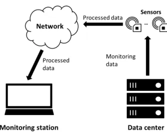
Consider a data center with hardware/software sensors recording performance-related data of the system as shown in Figure 1.1. The monitoring information may include hardware factors such as the runtime state of devices, software factors such as network activity within the data center and memory usage of virtual machines, and environmental factors such as the temperature at different locations. The collected information is then transmitted over a network to a monitoring station where data analysis and visualization are performed before the information is stored.
These measurements are important for making decisions on thermal systems and workload re-distribution of the data center. Therefore it is important that the collected information should reflect the real-time status of the data center. However, collecting these measurements has its costs. Sen-sors that add sensing-related code within the application code to monitor the performance-related data can easily interfere with the online application. Transmitting the collected information over the network consumes network bandwidth. Furthermore, if the sensors communicate with the mon-itoring station over a wireless network, both the act of collecting information at the sensors and transmitting the collected information over the wireless network consume power. Logging the data for future use, such as analysis aimed at capacity planning, consumes disk space. It is therefore desirable for the monitoring system to minimize the above-described costs.
As shown in Figure 1.2, there are two major categories of techniques for monitoring: monitor-ing with known correlation and monitormonitor-ing with unknown correlation. In monitormonitor-ing with known correlation, the relationship between performance-related measurements is assumed to be known and exploited to reduce the cost of monitoring. In monitoring with unknown correlation, the rela-tionship between performance-related measurements to be collected is unknown, and each one of the performance-related factors is monitored independently.
Figure 1.1: The system monitoring model in the case of monitoring a data center.
Figure 1.2: Categorization of methods for system monitoring and anomaly detection. The categories to which the proposed methods of this dissertation belong are enclosed in the dotted lines.
1.1.1 Monitoring with known correlation
In the first category of monitoring techniques, performance-related measurements are consid-ered as multiple variables that are correlated, and their correlation is assumed to be known prior to the monitoring. This correlated relationship is exploited during the data collection to reduce monitoring cost.
Consider a data center where environmental measurements (e.g., the fan temperature) and soft-ware/hardware factors (e.g., the CPU utilization and power usage of each machine) are collected at physically distributed remote sensors and then transmitted to a monitoring station for analysis. The monitoring factors are correlated. For example, temperature readings are similar at nearby lo-cations. When the CPU utilization of a machine is high, so is its fan temperature and power usage. The correlation between measurements can be exploited to reduce the cost associated with the data collection at each sensor as well as the cost associated with transmitting the data to the monitoring station.
Clustering is one of the methods that exploit the correlation between measurements to reduce the size of data transmitted over the network [7, 8, 9, 10]. This method divides sensors into subsets, and sensors whose measurements are correlated are put in the same subset. These subsets are also referred to as clusters. Within each cluster, one sensor is selected as the cluster head, and each sensor only needs to communicate to its cluster head. The cluster head is responsible for collecting the raw data, i.e., measurements from all the other sensors in its cluster, and sending the aggregated information to the monitoring station. Instead of using fixed cluster heads, techniques discussed in [11, 12, 13, 14] apply self-organization to dynamically assign a cluster head to each cluster.
The aggregation of the raw data performed by the cluster head exploits the correlation within the data to reduce information redundancy [15, 16]. Therefore, the size of the aggregated data is smaller than the overall size of the raw data collected by all the sensors. As a result, the size of the data transmitted over the network and then logged at the monitoring station can be reduced significantly by employing the clustering method.
The monitoring cost can be further reduced by reducing the cost associated with the data collec-tion at each sensor. For example, methods such as distributed compression [17, 18] and distributed
source coding [19, 20] can be employed at sensors within the same cluster to gather correlated data. It has also been proposed that some sensor nodes can be turned off, or go to sleep, to reduce sampling cost [21, 22].
1.1.2 Monitoring with unknown correlation
In the second category wherein the correlation between measurements is unknown, each of the performance-related measurements has to be collected independently. Without any assumption on the correlation between measurements, techniques in this category can be applied on a broader range of data. One straightforward method is to log the mean value of data over each fixed period of time. This method uses a sliding time window with a predetermined length, and records the mean of the monitored data within each time window. The series of mean values are then used for data analysis [23]. While it is easy to implement and requires low memory, this method has a few drawbacks. First, the output of averaging is sensitive to the window length. A larger window size leads to a smoother data series, while interesting data patterns within each time window get erased by the act of averaging. Besides, to calculate the mean, it is necessary to aggregate all the observed data within a time window. However, such aggregation is impractical for some applications. For example, inspecting every packet passing through each router of a backbone network for network traffic monitoring causes unacceptable delay [24].
One traditional strategy for monitoring is random sampling [25, 26], where each one of the data points is chosen to be collected with a probability that is predetermined by the sampling rate. Random sampling is widely used because it requires very little memory consumption and CPU power on the monitoring nodes. In the case of traffic monitoring, random sampling can be applied on the packets to examine the ongoing traffic without impairing the network traffic. However, the technique of random sampling can be biased for some applications [25]. When a monitoring system is used to estimate flow statistics, a router keeps the statistics of active flows that are passing through. The obtained result is useful for network monitoring and accounting, and helps identify anomalies in the network. Using random sampling, packets that belong to a larger traffic flow are more likely to be sampled than those which belong to a small flow. As a result, the estimated flow distribution using the randomly selected samples is biased toward larger flows. Data with such bias can lead to
incorrect decisions by network operators [27].
Sampling with priority is another technique used to remove the bias mentioned above [28]. Given an ultimate goal for monitoring, the sampling rate for each data series is adjusted based on the contribution of the data to the goal. For example, Meng et al. propose a method in [29] to detect violations that are defined as extreme values exceeding some threshold in the performance-related measurements of data centers. The sampling rate is updated dynamically: it is increased when the likelihood of detecting a violation is high, and decreased when the likelihood of detecting a violation is low. Similarly, Wanget al. propose the Residual-Geometric sampling for monitoring the distribution of network traffic flow at a router [30]. In this sampling strategy, a packet belonging to a new traffic flow is sampled with a predetermined probability, while packets belonging to the existing traffic flows are always sampled. The collected samples are then used to estimate traffic flow distribution, and the estimation result is more accurate than is possible with random sampling. The techniques of sampling with priority are, however, application specific, and it is difficult to extend them for other applications.
1.2 Resource-efficient system monitoring using compression and compressive sampling In this dissertation, we consider the following two methods for monitoring: compression and compressive sampling. These two methods are monitoring techniques with unknown correlations and therefore can be applied universally. In particular, compression is a non-sampling method, while compressive sampling is a sampling method. They have been widely applied for they allow a good reconstruction of the original data with small sample sizes.
1.2.1 Resource-efficient system monitoring using compression
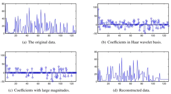
The system monitoring using compression involves five steps, as shown in Figure 1.3. The first four steps are implemented by the sensors, and the last step is carried out at the monitoring station. In the first two steps, the data is collected and then transformed into another basis. Next, the coefficients in the new basis that are the largest in magnitude are preserved as the compressed form of the original data. The compressed data is then sent to the monitoring station. In the final step,
Figure 1.3: The system monitoring model using compression. 20 40 60 80 100 120 0 20 40 60 80
(a) The original data.
20 40 60 80 100 120
−50 0 50 100
(b) Coefficients in Haar wavelet basis.
20 40 60 80 100 120
−50 0 50 100
(c) Coefficients with large magnitudes.
20 40 60 80 100 120 0 20 40 60 80 (d) Reconstructed data.
Figure 1.4: The form of data at different stages of the monitoring model using compression. (a) the original data to be collected. (b) the representation of the data in the Haar wavelet basis. (c) the compressed form of the data after applying thresholding on the coefficients. (d) the reconstructed data after applying inverse wavelet transform on the compressed form of data.
inverse transform is applied on these coefficients to approximate the original data. An example of the data at different stages of this monitoring model is shown in Figure 1.4.
The technique of compression exploits the property of sparsity, which shows how concisely the data can be expressed in one basis [31]. Under the basis in which the data is more sparsely repre-sented, fewer coefficients need to be preserved in the compressed form. Therefore, it is desirable to find a basis in which the data to be collected is sparse.
Figure 1.5: The system monitoring model using compressive sampling
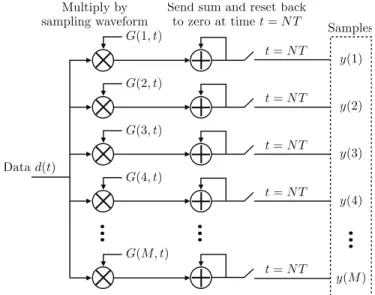
1.2.2 Resource-efficient system monitoring using compressive sampling
Compressive sampling, also known as compressive sensing or compressed sensing, is a sam-pling technique that guarantees accurate reconstruction of sparse data from only a small amount of samples [32]. Similar to compression, a compressed form of the original data is obtained in the sampling process. However, the sampling process of compressive sampling is simply multiplying the original data in the form of a vector with a sensing matrix. Besides, the number of the resulting samples is far fewer than the length of the original data. Reconstruction algorithms are applied on the obtained samples to approximate the original data. A class of reconstruction algorithms called basis pursuit or iterative hard thresholding pursuit (HTP) [33] is used to reconstruct the original data. The model of monitoring using compressive sampling consists of three steps, as shown in Figure 1.5. In the first two steps, the sensors sample the data in a compressed form and send the compressed data to the monitoring station. In the final step, the monitoring station applies the re-construction algorithm to recover the original data from the samples. Using the same original data as in Figure 1.4, we show in Figure 1.6 the compressed form of data and the reconstructed data in the monitoring model using compressive sampling.
Two sets of bases, the sensing basis and the representation basis, are used in compressive sam-pling. The sensing matrix for collecting the data is composed of the sensing basis, and the represen-tation basis is for representing the data. The compressive sampling theory is based on two properties associated with these two bases, the sparsity property of the data in the representation basis and the property of incoherence between the sensing basis and the representation basis. The sparsity prop-erty allows the data to be sparsely represented in the representation basis. When the sensing and representation bases are uncorrelated or incoherent, a spike in one basis will be represented as a
5 10 15 20 25 30 −5000
0 5000
(a) Compressed samples.
20 40 60 80 100 120 0 20 40 60 80 (b) Reconstructed data.
Figure 1.6: The form of data at different stages of the monitoring model using compressive sam-pling. The original data is the same as in Figure 1.4. (a) the sampled data that is also in the com-pressed form. (b) the reconstructed data after applying reconstruction algorithm on the comcom-pressed form of data.
spread-out waveform in the other. For example, the Dirac delta basis and the Fourier basis are incoherent. In this case, data shown as a spike in the Dirac basis is spread out when represented in the Fourier basis. When the sensing and representation bases are incoherent, using the sensing basis to sample the data that is sparsely represented in the representation basis is also referred to as incoherent sampling. The property of incoherence allows us to capture the useful information content embedded in the data and condense it into a small amount of data by incoherent sampling.
Reconstruction of the original data using HTP is considered to be exact with high probability if the sample size is greater than a lower bound defined by the sparsity and the coherence [34]. Typi-cally, when the coherence as well as the sparsity are small, we need only a few samples to recover the original data exactly with high probability. It is therefore desirable to find a representation basis in which the data to be collected is sparse and a sensing basis that has small coherence with the representation basis.
1.2.3 Comparing compression and compressive sampling
Both compressive sampling and compression exploit the sparsity property. Since the sample size as a result of compression and compressive sampling is small, the network bandwidth required to transmit the samples to the monitoring station is reduced and so is the hard-disk space required to store them. When operators wish to analyze the original data, there is a way to use numerical optimization to reconstruct the full-length data from the sample set. However, these two methods are fundamentally different.
In compression, the original data is transformed into the representation basis, and the obtained coefficients are sorted to get the compressed form of the original data. The sampling process of compressive sampling, which is multiplying the data with a sensing matrix to obtain the compressed form, is comparatively simpler with a smaller sampling overhead. As a result, the simple sampling process of compressive sampling can significantly reduce the intrusion of monitoring on the system. The sample size as a result of compressive sampling, nonetheless, can be larger than that of com-pression. The reconstruction of compressive sampling is more complex compared with the inverse transformation employed by compression.
1.3 Anomaly detection
Anomaly detection is a technique that can detect attacks and unusual states of a system. It has been widely applied in system monitoring, such as intrusion detection in a network [35] and in a cloud computing environment [36]. Anomalies are data patterns that do not conform to a well de-fined notion of normal behavior. These anomalous patterns are usually caused by malicious attacks on a network (e.g., denial-of-service (DoS) attacks, port scans), system breakdown, or measurement faults. For example, a DoS attack can lead to a sudden increased number of requests to one server. The occurrence of a hardware fault in one single machine can lead to run-time computing failures in the cloud computing system. Many of these anomalies can be a threat to the health of a system. It is critical for system operators to apply anomaly diagnosis to detect these unusual patterns promptly and accurately, and identify the irregularities automatically.
Anomaly detection along with anomaly identification and classification constitute anomaly di-agnosis, as shown in Figure 1.2. Anomaly identification and classification are also known as root cause analysis. Anomaly detection systems monitor performance-related features and send alarm messages whenever an abnormal change of any kind is observed. Root cause analysis tries to clas-sify the anomaly based on characteristics of the anomalous pattern and identify the underlying cause.
Intuitively, anomaly detection seems no more difficult than performing a comparison: use exist-ing statistical-analysis techniques to compare the performance-related measurements with a
statisti-cal model of normal behavior, and generate an output if there exist any statististatisti-cal outliers. However, there are many pitfalls in this intuition. First, it is difficult to get statistical definitions of normal behaviors. Traffic of a backbone network, for example, varies significantly all the time, and change of settings at the routers can lead to different traffic patterns. Besides, the normal behavior of a system keeps evolving all the time, thus it may take a long time to find a normal pattern. Even if we have a model for the normal pattern, the detection result is sensitive to detection settings such as the boundary between normal and abnormal behaviors. Furthermore, limitations on available measurements will degrade the performance of an anomaly detection system.
With these challenges, two basic categories of techniques have been developed for anomaly detection as shown in Figure 1.2: signature-based and statistic-based.
1.3.1 Signature-based techniques for anomaly detection
Signature-based techniques detect anomalies by looking for a pattern that matches signatures of known anomalies [36]. In [37], Feather et al. use a signature matching mechanism to detect failures of an Ethernet network. Moore et al. use the property of address uniformity in several popular DoS toolkits to diagnose DoS in [38]. Violation detection in data centers detects anomalies that are defined as extreme values exceeding a threshold [29]. Many software systems and toolkits for network security, such as Bro and Snort proposed in [39] and [40], have been developed based on signature-based techniques. However, techniques in this category have the limitation that they can only detect the known anomalies and thus compromise system security when some unknown anomalies occur in the system.
1.3.2 Statistic-based techniques for anomaly detection
The statistic-based techniques do not require any prior knowledge about the anomalies. Instead, techniques in this category look for significant changes in short-term statistics of performance-related data. Therefore, these techniques are also referred to as change detection and can be effective for both known anomalies and unknown anomalies. Based on the type of anomalies they target, the methods in this category can be divided into two subtypes: volume anomaly detection and pattern anomaly detection.
1. The techniques for volume anomaly detection are the methods that detect unusual volume changes in the univariate data. Many methods have been proposed to apply statistical tech-niques to detection volume anomalies. For example, Barfordet al. treat anomalies as devi-ations in the overall traffic volume, and use the traffic variances at different time-frequency scales to distinguish predictable and anomalous traffic volume changes [41]. It has been pro-posed to apply a variety of time series forecast models (e.g., ARIMA and Holt-Winters) on network traffic, and look for traffic flows with large forecast errors to detect traffic anoma-lies [42, 43, 44, 45]. For example, the AnomalyDetection R package tool recently released by Twitter on GitHub [45] aims to detect anomalies in time series data. This tool assumes a smooth transition in normal data series such as activities of uploading photos on Twitter, and uses seasonal hybrid extreme studentized deviate (S-H-ESD) test to quantify deviation of a datapoint from its prediction. Datapoints that deviate from their predictions are flagged as anomalies in seasonal univariate time series. This tool is able to detect both global and local anomalies that do not necessarily appear to be extreme values.
2. The techniques for pattern anomaly detection are the methods that detect unusual patterns in the multivariate data. In particular, these techniques explore correlations between differ-ent measuremdiffer-ents and detect anomalies by checking changes of correlation. For example, Lakhinaet al.propose to apply PCA in [46] to explore anomalous deviations in the distribu-tion of network-wide traffic, and use the deviations to signal, identify and classify anomalies. Lan et al.[47] employ PCA and independent component analysis (ICA) to extract features from the data of large-scale systems, apply unsupervised learning on the extracted features, and identify anomalous nodes of the system as the nodes acting differently from the others. Guanet al.propose in [48] to exploit the most relevant principal components (MRPCs) to de-scribe system failures in cloud computing infrastructures, and adaptively identify the detected anomalies.
Figure 1.7: Principal components of two-dimensional data.
1.3.3 Principal component analysis for anomaly detection
PCA is a technique for dimension reduction which is widely used for anomaly detection in network [46, 49, 50, 51], cloud computing infrastructure [48, 52] and other large-scale systems [47]. Given a set of observations that are high-dimensional, applying PCA on the data gives us a set of orthogonal axes, which are called principal components and along which the observations are correlated. Furthermore, these principal components are ordered by the strength of correlation the data exhibits along their directions. The correlation captured by each principal component is quantified by the variance of the data along its direction. As a result, the first principal component captures the strongest correlation between the features, the second principal component captures the second strongest, and so on [53]. Figure 1.7 shows two principal components, PC1 and PC2, as the result of applying PCA on a two-dimensional dataset. The first principal component, PC1, gives us the direction along which the data is most correlated.
The performance-related data of a system are inevitably correlated. For example, a correlation exists between the traffic passing through two neighboring routers. The thermal readings at different nodes in a sensor network are correlated, and the readings at two nearby nodes are similar. The response time of an application server is correlated with the CPU utilization of the machine that hosts the application. Because of such correlations, the number of principal components that capture the major patterns is usually smaller than the dimension of the original dataset. As a result, we are able to reduce the dimension of highly correlated datasets and thus reduce the complexity of data analysis by employing PCA.
com-plete set of principal components. Then, a set of principal components are selected such that they account for a certain amount of variance exceeding a predetermined threshold [47, 49, 50, 51, 52]. In [49], the principal components that are chosen as the extracted features form thenormal subspace, and theanomalous subspaceis composed of the rest of the principal components. An underlying assumption in [49] is that anomalies exhibit correlations that are different from those captured by the normal subspace. Based on this assumption, the projection of data without anomalies onto the normal subspace should be large, while its projection onto the anomalous subspace should be small. Similarly, the projection of anomalous data onto the anomalous subspace should not be small. The anomaly detection is implemented by projecting the test data onto the anomalous subspace, and sending an alert if the projection is above a threshold. This method of applying PCA to construct normal and anomalous subspaces for anomaly detection is referred to as thesubspace method.
1.4 Contribution to resource-efficient monitoring
As shown in Figure 1.2, one part of this dissertation is to develop two simple yet effective mon-itoring tools. One of the monmon-itoring tools is based on compression, a non-sampling technique. We term this monitoring tool as C-MON. The other monitoring tool called CS-MON employs compres-sive sampling, a sampling technique. The technique of compression and comprescompres-sive sampling are for monitoring with unknown correlation, and thus our monitoring tools can be applied to monitor each one of the performance-related measurements. With no assumption on the correlation between the monitored data, these tools can be applied for general purposes.
1.4.1 C-MON: monitoring using compression in the best basis
In C-MON, compression is applied on performance-related measurements, and the compressed form of the data is sent to the monitoring station for data analysis. Note that the data can be rep-resented at different sparsity levels under different bases. In Figure 1.8, we show that the sparsity of a dataset is different in two wavelet bases. For the basis in which the data is more sparsely rep-resented, fewer coefficients need to be preserved in the compressed form. Using the same sample size, both compressive sampling and compression can reconstruct the data with greater fidelity if
20 40 60 80 100 120 2050
2100 2150 2200
(a) The original data
20 40 60 80 100 120
−50 0 50 100
(b) In Haar wavelet basis.
20 40 60 80 100 120 0 5000 10000 15000 (c) In db2 wavelet basis.
Figure 1.8: The sparsity of data in (a) in two wavelet bases: Haar and db2. (a) An example of data series reflecting the memory allocated to a virtual machine. (b) Representation of the data in Haar wavelet basis. (c) Representation of the data in db2 wavelet basis. The data is more concisely represented in the db2 basis.
we know beforehand the underlying basis in which the data is sparse.
Selecting the appropriate basis under which the measured data is most sparse requires some experimentation using representative training data from the system. We propose to employ a basis selection strategy,best basis algorithm, that reduces this burden on the system operator by automat-ically adapting the representation basis to the structure of the sampled data.
In our design, the best basis should satisfy two conditions. First, the representation of the data in this basis should be sparse. Second, the approximation error as a result of using the compressed form of the data in this basis should be small. Considering these two conditions, we formulate a cost function associated with each candidate basis. There are two terms in this cost function, one for the sparsity and the other for the approximation error [54]. We then choose the best basis as the one that minimizes the cost function.
The system monitoring model of C-MON is shown in Figure 1.9. Comparing with the compression-based monitoring model in Figure 1.3, C-MON has an additional component which implements the best basis strategy. Given a set of candidate bases, C-MON employs the best basis strategy to find the basis in which the data can be most sparsely represented. The data is then compressed in this best basis so that the size of data in its compressed form is the smallest. As a result, the network traffic for sending the monitored information to the monitoring station is reduced by employing the best basis strategy.
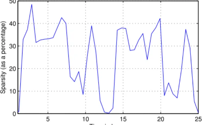
Figure 1.9: The system monitoring model of C-MON. 5 10 15 20 25 0 10 20 30 40 50 Time in hours
Sparsity (as a percentage)
Figure 1.10: Change in the sparsity level over time for the measurement of memory usage of a virtual machine in a data center.
1.4.2 CS-MON: monitoring using adaptive-rate compressive sampling
The other monitoring tool we develop in this dissertation, termed CS-MON, applies the tech-nique of compressive sampling on the data.
The technique of compressive sampling has been widely used for cognitive radio [55, 56, 57, 58], MRI [59, 60, 61, 62], radar imaging [63, 64, 65, 66] and video coding [67, 68, 69] for the underlying sparsity property of the data. It has been rarely used for system monitoring except in [70] for the monitoring of wireless sensor networks, in [71] for the monitoring of power systems, and in [72] for the monitoring of data centers.
In works that apply compressive sampling for system monitoring (e.g., [72]) the sparsity of the data when represented in the underlying basis is assumed to be constant or bounded over time. Under such an assumption, one can use a fixed rate for sampling the data. This assumption of a constant sparsity, however, rarely holds in practice. For example, we measure the memory usage of a virtual machine in our case study of monitoring a data center. In particular, the data records the
Figure 1.11: The system monitoring model of CS-MON.
amount of memory allocated by processes in the system using malloc() calls. We find this data to be sparse in Haar wavelet basis, and plot in Figure 1.10 the sparsity of the data during a 25-hour period. The sparsity is defined as the percentage of coefficients needed within the Haar wavelet basis to capture 99% of the information contained within the data. The sparsity of the data varies significantly over time. So a simple sampling strategy, say one that chooses a fixed rate based on an upper bound on the sparsity level—between 45-50% in this particular case—incurs a large sample size. We can perform much better in terms of reducing the number of samples needed by dynamically increasing or decreasing the sampling rate as the sparsity changes.
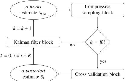
In this dissertation, we improve the compressive sampling strategy in Figure 1.5 by adding a rate adjustment component inspired by the work in [73]. The flow chart for CS-MON, the system monitoring tool using adaptive-rate compressive sampling, is shown in Figure 1.11. Our idea is that by collecting some relevant side information from the data—which could have been under or over sampled during any particular time window—we can estimate the underlying sparsity and predict it for some succeeding time windows. The number of samples collected over these succeeding windows can then be adjusted based on the predicted sparsity values. Our goal is to achieve an overall reduction in sample size without compromising the reconstruction quality.
We apply CS-MON strategy for online monitoring of a data center as a case study. In particular, we show that to achieve the same reconstruction quality, this monitoring strategy is able to reduce the sample size by 70% compared with constant-rate compressive sampling. We also use the recon-structed data of compressive sampling for two cases of anomaly detection: violation detection and trend detection.
1. Violation detection. Violations are defined as values that exceed some threshold. These viola-tions are usually performance-related bottlenecks or anomalies. We use the metric of hit rate to evaluate the performance of CS-MON. Here, a hit is defined as a spike in the reconstructed data that matches a similar spike in the original data. Our result shows that this strategy is able to achieve 90% hit rate using about 30% of the original data.
2. Trend detection. A decreasing or increasing trend in the data can reflect performance dete-rioration associated with software aging or resource exhaustion. We use a linear model to fit the reconstructed data, and detect the trend by checking the estimated slope of the linear model. Our result shows that using around 30% of the original data, we are able to detect the increasing trend in the measurements collected from our testbed with high confidence.
1.5 Contribution to anomaly detection
1.5.1 Anomaly detection with compressed measurements
Compressive sampling used in the aforementioned CS-MON allows for a very simple sampling strategy on the local machine. When operators wish to analyze the original signal, there is a way to use numerical optimization to reconstruct the full-length signal from the sample set. The recon-structed signal allows for real-time anomaly detection and diagnosis, and also helps drive decisions of a longer-term nature such as intelligent capacity planning. The recovery process is typically posed as a linear programming (LP) problem and solved under some sparsity assumptions using a class of reconstruction algorithms called basis pursuit or iterative hard thresholding pursuit [33]. Though modern LP solvers are quite efficient, each monitoring station may be responsible for recov-ering and analyzing hundreds of signals belonging to many servers, making it important to reduce the corresponding overhead.
We propose to apply anomaly detection directly on compressed measurements to reduce the computational cost incurred by the monitoring station, associated with recovering the original signal from the sample set and analyzing it for anomalies. Our work makes the following contributions towards this goal:
prop-erties of the original data such as variance and mean. This result allows for the detection of abrupt changes and trends bydirectly analyzingjust the compressed samples without having to reconstruct the full-length signal.
• Since the sampling process is just a linear projection of the original data, we also prove that the compressed samples approximatelypreserve spectral propertiessuch as correlation between data points, the length of the data vectors, as well as the distance between two vectors, under such a projection. This result allows for well-known anomaly detection methods such as PCA to be used directly on the compressed samples; performance is almost equivalent to the case in which the raw data is completely available.
We illustrate the usefulness of the approach via case studies using IBM’s Trade Performance Benchmark (also known as Trade6). We measure signals from the disk and memory subsystems us-ing a CS-based samplus-ing strategy, and analyze the compressed samples for possible anomalies. The first scenario involves detecting abrupt changes in the signal during which the magnitude exceeds some nominal threshold value. In the second scenario, we wish to detect the gradual deterioration of system performance, say over hours or days, associated with software aging by statistically an-alyzing the appropriate signals for the existence of trends [74, 75]. We use a long-running Trade6 application having a small memory leak and evaluate the ability of the approach to estimate a posi-tive slope in the compressed data even in the presence of seasonal variations and periodicity in the signal. Finally, we evaluate the efficacy of applying PCA to the compressed samples to detect abrupt changes in the signal.
Abrupt changes can be detected using a sample size of 25% with a hit rate of 95% for a fixed false alarm rate of 5%; trends can be detected with a confidence interval of 95% using a sample size of 6%. Finally, the hit rate achieved by the PCA-based analysis when using the compressed samples to detect abrupt changes is higher than 95% when the false alarm is fixed at 0.5%. The corresponding sample size is about 18%. These results point to the feasibility of adopting a two-step anomaly detection process at the monitoring station: the received compressed data is examined for possible anomalies; if one is suspected, the relevant portion of the signal is fully reconstructed to localize and further analyze the anomaly.
1.5.2 Anomaly detection with the maximum subspace distance
The subspace method proposed in [49] has been widely applied and is shown to be effective in detecting anomalies for traffic monitoring [49] and for cloud computing security [52]. However, this method has the following drawbacks [51, 76]: the detection rate of the method is sensitive to the chosen dimension for the normal subspace, and anomalies that reside within the normal subspace will be missed by the detection tool.
As mentioned earlier, PCA is applied on a set of training data and then the most dominant prin-cipal components are selected to form the normal subspace. The dimension of the normal subspace, or the number of principal components, is selected such that it accounts for a predetermined amount of variance in the training dataset. In this way, the detection tool proposed in [49] is able to detect anomalies that do not comply with the correlations captured in the normal subspace. As a result, the range of anomalies that can be detected relies on the training data and user input of threshold for the variance that should be captured by the normal subspace. In the following, we refer to this method as thevariance-based subspace method.
Considering these drawbacks associated with the variance-based subspace method, we propose a new metric namedsubspace distanceto differentiate between two behavior datasets of a system, and use this metric to detect changes in correlation patterns. More importantly, we show that the value of our proposed metric explains the significant correlation changes, if any, between the measured data and the training data. Consequently, this metric provides more information about the detected anomalies.
We choose the second-order statistics, the covariance matrix, to summarize a system behavior. By using the covariance matrix, we place no prior assumption on the distribution of measured data. Besides, the result in [77] shows that anomalies lead to changes in the covariance matrix and that the deviations in a covariance matrix corresponding to different anomalies are different. Inspired by work in [77], we aim to develop a general metric to quantify the difference between two covariance matrices, and use the measured difference to detect and identify anomalies.
The subspace distance is calculated as follows. After applying PCA on the two covariance matrices, one for each of the system behaviors, we obtain two sets of principal components. We
(a) Two sets of subspaces (b) The subspace angle.
Figure 1.12: The example of subspace distance between two sets of principal components. (a) Two sets of principal components: {a1,a2}and{b1,b2}. (b) The subspace angle between a pair of subsets of principal components when the number of principal components included in each subset increases from 0 to 2. The subspace angle is maximum when the subspace dimension is 1. The maximum subspace angle isθ, i.e., the angle betweena1andb1.
then choose a subset from each set of principal components, and calculate the angle between these two subsets. The subspace distance is the maximum angle between any pair of subsets of principal components. The two subsets of principal components corresponding to the maximum angle are the signature patterns of these two system behaviors. In the example shown in Figure 1.12,{a1,a2}and {b1,b2}are the principal components of two system behaviors. The maximum subspace angle isθ, the angle between{a1}and{b1}. As a result, the subspace distance between these two behaviors is
θand is achieved when{a1}and{b1}are chosen as the signature pattern of each behavior.
Particularly, the metric of subspace distance quantifies the difference between correlation pat-terns of two system behaviors. These two behaviors can be the normal and anomalous behaviors of a system, in which scenario the metric quantifies the anomalous change in the system behavior. They can also be the behaviors of a system at different stages, in which scenario the metric quantifies the change of system status.
Given two system behaviors, one during the training phase and the other one during the test phase, we derive the maximum subspace distance and obtain two subsets of principal components corresponding to the maximum subspace distance. We then examine these two subsets of prin-cipal components for the significant correlation change caused by anomalies occurred during the test phase. We refer to this method as thedistance-based subspace method. In the following, we present two efficient algorithms that allow us to obtain information about the correlation changes in centralized and decentralized scenarios.
The centralized algorithm for subspace distance estimation
The definition of our proposed subspace distance shows that two complete sets of principal components need to be calculated first. However, it can be computationally expensive to calculate principal components for datasets with high dimensions (e.g., network flow data from each source IP address can have up to 232 dimensions). We propose an efficient algorithm that estimates the subspace distance with much lower computational complexity.
The key ideas of our proposed algorithm are listed below.
1. Reduction of search range. The subspace distance is found by comparing pairs of subsets of principal components. We prove that the searching range can be reduced fromO(N2) to O(N), whereNis the dimension of the measurements.
2. Using only a subset of principal components. Instead of calculating two complete sets of prin-cipal components, we choose to calculate one prinprin-cipal component for each dataset at a time using the power iteration method [78]. The order for calculating the principal components is the same as the significance of these principal components.
3. Simplified computation of subspace angle. We develop a simplified procedure of computing the subspace angle between any pair of subsets of principal components.
4. Setting a stop condition for searching. To avoid calculating two complete sets of principal components, we set a stopping condition for the search of subspace distance. We prove that the stop condition of our algorithm can get us an approximation of the subspace distance with bounded error.
We validate each of these ideas with mathematical proofs and experimental results. We then de-velop a centralized algorithm based on these ideas. We show that the estimated subspace distance as a result of our algorithm is close to the actual subspace distance with significantly lower complexity. The decentralized algorithm for subspace distance estimation
The data required for computing covariance matrices is usually collected at physically dis-tributed nodes, such as network traffic at different routers and temperature readings at different
sensor nodes. In order to perform the centralized algorithm, a data sink is required to collect all the data from the collection nodes, compute covariance matrices, and run the algorithm.
In a distributed mode where there is no such data sink, a collection node will need to collab-orate with its neighbors to estimate principal components in a distributed fashion. In this setting, the covariance matrix is unknown to each node, and the power iteration method for calculating the principal components has to be implemented in a distributed manner. We propose that this is fea-sible with Gaussian gossiping [79, 80]. In the decentralized algorithm, each node will only need to communicate information with its neighbors and estimate its corresponding entry in the princi-pal components instead of computing the complete vectors of principrinci-pal components. With partial knowledge about the principal components, each node can compute the subspace angle in a dis-tributed fashion and collaborate with its neighbors to estimate the subspace distance. We derive the tradeoffbetween the accuracy of the estimation and the volume of communications among the sensing nodes as a result of our decentralized algorithm.
2. An Efficient Strategy for Online Performance Monitoring of Datacenters via Adaptive Sampling
Performance monitoring of datacenters provides vital information for dynamic resource provi-sioning, anomaly detection, capacity planning and metering decisions. Online monitoring, however, incurs a variety of costs: the very act of monitoring a system interferes with its performance, con-suming network bandwidth and disk space. With the goal of reducing these costs of online moni-toring, this chapter develops and validates a strategy based on adaptive-rate compressive sampling. It exploits the fact that the signals of interest often can be sparsified under an appropriate represen-tation basis and that the sampling rate can be tuned as a function of sparsity. We use the Trade6 application as our experimental platform and measure the signals of interest—in our case, signals pertaining to memory and disk I/O activity—using adaptive sampling. We then evaluate whether the reconstructed signals can be used for trend detection to track the gradual deterioration of sys-tem performance associated with software aging. Our experiments show that the signals recovered by the our methods can be used to detect, with high confidence, the existence of trends within the original signal. We also evaluate the reconstructed signals for threshold-violation detection wherein the magnitude of the signal exceeds a preset value. Our experiments show that performance bottle-necks and anomalies that manifest themselves in portions of the signal where its magnitude exceeds a threshold value can also be detected using the reconstructed signals. Most importantly, detection of these anomalies is achieved using a substantially reduced sample size—a reduction of more than 70% when compared to the standard fixed-rate sampling method. The material presented in this chapter was previously published in [81, 82, 83].
2.1 Introduction
Online performance monitoring of both the IT infrastructure and the physical facility is vital to ensuring the effective and efficient operation of datacenters [84, 85]. Examples of monitoring solutions include the Tivoli Monitoring software from IBM for the IT infrastructure [86] and the
Datacenter Environmental Edge from HP that monitors temperature, humidity, and state of the power network within the datacenter. The monitored information has a variety of uses. It supplies the metering data used by pay as you use pricing models for cloud resources. It also drives real-time performance management decisions such as dynamic provisioning of IT resources to match the incoming workload, detection and mitigation of performance-related hotspots and bottlenecks, and fault diagnosis. In the case of intermittent problems that are hard to isolate, browsing back through historical data can help identify and localize recurring problems affecting the same portion of the IT infrastructure at different times. The monitored information also drives decisions of a longer-term nature; for example, intelligent capacity planning that identifies resources that are over-utilized or under-utilized and aims to improve utilization by adding or removing appropriate resources.
We consider a server cluster wherein software-based sensors embedded within the IT infrastruc-ture measure various performance-related parameters associated with the cluster. These measure-ments include high-level metrics such as response time and throughput as well as low-level metrics such as processor utilization, I/O, memory, and network activity. The information collected by the sensors is transmitted over a network to a monitoring station for data analysis and visualization. On-line monitoring, however, incurs a variety of costs. First, the very act of monitoring an application interferes with its performance. If sensing-related code is merged with the application code, this change may interfere with the timing characteristics of the application or if sensors execute as sepa-rate processes, they contend for CPU resources along with the original application. Transmitting the monitored data over a network consumes bandwidth. Finally, logging the data for futur