Evolutionary Many-objective Optimization of
Hybrid Electric Vehicle Control: From General
Optimization to Preference Articulation
Ran Cheng, Tobias Rodemann, Michael Fischer, Markus Olhofer, and Yaochu Jin,
Fellow, IEEE
Abstract—Many real-world optimization problems have more than three objectives, which has triggered increasing research interest in developing efficient and effective evolutionary algo-rithms for solving many-objective optimization problems. How-ever, most many-objective evolutionary algorithms have only been evaluated on benchmark test functions and few applied to real-world optimization problems. To move a step forward, this paper presents a case study of solving a many-objective hybrid electric vehicle controller design problem using three state-of-the-art algorithms, namely, a decomposition based evo-lutionary algorithm (MOEA/D), a non-dominated sorting based genetic algorithm (NSGA-III), and a reference vector guided evolutionary algorithm (RVEA). We start with a typical setting aiming at approximating the Pareto front without introducing any user preferences. Based on the analyses of the approximated Pareto front, we introduce a preference articulation method and embed it in the three evolutionary algorithms for identifying solutions that the decision-maker prefers. Our experimental results demonstrate that by incorporating user preferences into many-objective evolutionary algorithms, we are not only able to gain deep insight into the trade-off relationships between the objectives, but also to achieve high-quality solutions reflecting the decision-maker’s preferences. In addition, our experimental results indicate that each of the three algorithms examined in this work has its unique advantages that can be exploited when applied to the optimization of real-world problems.
Index Terms—Many-objective optimization, hybrid electric vehicle, preference articulation, reference vector, evolutionary algorithm
I. INTRODUCTION
M
ANY real-world optimization problems involve more than one conflicting objective to be optimized, known as multiobjective optimization problems (MOPs) [1]–[3]. Gen-erally, a minimization MOP can be formulated as follows:minimize f(x) = (f1(x), f2(x), ..., fM(x))
s.t.x∈X, f ∈Y (1)
Ran Cheng was with the Department of Computer Science, Univer-sity of Surrey, Guildford, Surrey, GU2 7XH, United Kingdom (e-mail: [email protected]). R. Cheng is now with the CERCIA group, School of Computer Science, University of Birmingham, United Kingdom.
Yaochu Jin is with the Department of Computer Science, Univer-sity of Surrey, Guildford, Surrey, GU2 7XH, United Kingdom (e-mail: [email protected]). Y. Jin is also with the College of Information Sciences and Technology, Donghua University, Shanghai 201620, P. R. China. (Corresponding author: Yaochu Jin)
Tobias Rodemann and Markus Olhofer are with the Honda Re-search Institute Europe GmbH, 63073 Offenbach, Germany (e-mail: {tobias.rodemann;markus.olhofer}@honda-ri.de).
Michael Fischer is with Honda R&D Europe Germany GmbH, 63073 Offenbach, Germany (email: michael [email protected])
whereX⊂RnandY ⊂RM are known as the decision space
and objective space, respectively, with x= (x1, x2, ..., xD)∈
X and f ∈ Y denoting the decision vector and objective vector in the two spaces,DandM are the number of decision variables and the number of objectives, respectively. Due to the conflicts between different objectives as formulated in (1), there does not exist one single solution that is able to optimize all objectives simultaneously. Instead, a set of solutions, known as the Pareto optimal solutions, can be achieved as the trade-offs between different objectives. To be specific, the Pareto optimal solutions are also known as the Pareto set (PS) in the decision space, while its image in the objective space is also known as the Pareto front (PF).
Evolutionary computation (EC) is one of three main areas of computational intelligence and various powerful evolutionary algorithms (EAs) for solving complex optimization problems have been developed. EAs, which are population based meta-heurisic search methods, are well suited for multiobjective optimization that are able to achieve a set of solutions in one single run. As most popular multiobjective evolutionary algorithms (MOEAs), e.g., the elitist fast non-dominated sort-ing genetic algorithm (NSGA-II) [4], the improved strength Pareto evolutionary algorithm (SPEA2) [5], a region based selection algorithm (PESA-II) [6], among many others [7], were originally proposed for solving MOPs which involve two or three objectives, the performance of these MOEAs deteriorates seriously when the number of objectives becomes more than three [8]–[11]. Nowadays, MOPs with more than three objectives are often called many-objective optimiza-tion problems (MaOPs) [12], which pose great challenges to traditional MOEAs for several reasons [13], [14]. First, as the number of objectives increases, an increasing number of candidate solutions will become non-dominated to each other, seriously degrading the performance of Pareto dominance based MOEAs due to the loss of selection pressure. Second, due to the large volume of the high-dimensional objective space, striking a good balance between convergence and di-versity becomes particularly important for the performance of MOEAs. Third, in order to approximate the high-dimensional PFs, the required number of candidate solutions increases exponentially. Other challenges include visualization of high-dimensional PFs and performance measurements of solution sets. In order to enhance the performance of MOEAs on MaOPs, various approaches have been proposed in recent years, which can be roughly categorized into the following three classes.
The first class is to enhance the convergence capability of traditional MOEAs. Among various convergence enhance-ment approaches, dominance modification is the most intuitive one. Examples of modified dominance definitions include L -optimality [15],-dominance [16], [17], fuzzy dominance [18], and grid based dominance [19]. Another typical idea of this category is to introduce new convergence metrics in addition to traditional dominance based mechanisms. For example, a shift-based density estimation strategy is proposed to penal-ize poorly converged solutions that cannot be distinguished by Pareto dominance [20]; a knee point based secondary selection is introduced on top of non-dominated sorting to enhance convergence pressure in the recently proposed knee point driven evolutionary algorithm (KnEA) [21]. Some other recent work along this line includes the two-archive algorithm for objective optimization (Two Arch2) [22], many-objective evolutionary algorithm based on both many-objective space reduction and diversity enhancement (MaOEA-R&D) [23], and the recently proposed bi-criterion evolutionary algorithm (BCE) [24].
The second class is decomposition based MOEAs where a complex MOP is decomposed into a number of simpler subproblems that are subsequently solved collaboratively [25], [26]. Decomposition based MOEAs can be further categorized into two groups [27]. The first class decomposes an MOP into a group of single-objective problems (SOPs), such as dynamic weighted aggregation (DWA) [28], cellular multi-objective ge-netic algorithm (C-MOGA) [29] and multi-objective evolution-ary algorithm based on decomposition (MOEA/D) [25]. The second class decomposes an MOP into a group of sub-MOPs, such as MOEA/D-M2M [26] and MOEA/DD [30], which are variants of MOEA/D, a variant of II, termed NSGA-III [31], an MOEA using Gaussian process based inverse modeling (IM-MOEA) [32], [33] and a recently proposed reference vector guided evolutionary algorithm (RVEA) [34]. It is worth noting that NSGA-III can be also seen as a Pareto dominance based MOEA, since the primary selection in NSGA-III is still non-dominated sorting.
The third class is performance indicator based MOEAs. Performance indicators are originally designed to evaluate the quality of solution sets but later found to be useful as a selection criterion in MOEAs. Representative algorithms of this class include the S-metric selection based evolutionary multi-objective algorithm (SMS-EMOA) [35], the indicator based evolutionary algorithm (IBEA) [36] and the fast hyper-volume based evolutionary algorithm (HypE) [37]. Although this class of MOEAs do not suffer from dominance resistance, unfortunately, the computational cost for indicator calculation becomes prohibitively as the number of objectives increases [38]–[40].
In spite of the various MOEAs in the literature, research on evolutionary many-objective optimization is still in its infancy and there is a big gap between academic research and demand from industry for the following main reasons. First, most algo-rithms have merely been assessed on benchmark test problems
for general optimization1, where the performance is mostly evaluated using performance indicators originally proposed for multiobjective optimization with two or three objectives. Second, most MOEAs proposed for many-objective optimiza-tion are meant to achieve a representative approximaoptimiza-tion to the PF. By contrast, in real-world MaOPs, it is particularly useful if an algorithm is able to incorporate preferences of DMs [12], where the approximation of high-dimensional PFs with a limited number of solutions becomes impractical. Thus, there is a strong need to demonstrate the capability of the MOEAs proposed for solving real-world MaOPs.
To bridge the gap between academic research and industrial applications, this paper presents a case study where three state-of-the-art MOEAs, namely, MOEA/D [25], NSGA-III [31], and RVEA [34] are employed to solve a seven-objective optimization problem in hybrid electric vehicle (HEV) control. By proposing a generic preference articulation method, we demonstrate that the three algorithms are not only able to perform general optimization, but also capable of identifying optimal solutions preferred by the decision maker (DM). The main new contributions of this work can be summarized as follows.
1) The paper exemplifies a successful application of MOEAs for real-world many-objective optimization. As previously mentioned, most MOEAs have only been as-sessed in general optimization on benchmark test prob-lems using performance indicators. In practice, however, it is more useful if user preferences can be articulated in the optimization process. In this case study, we illustrate how existing MOEAs can meet such demands in the optimization of a seven-objective HEV controller design problem.
2) As an extension of our previous work [41], this pa-per details a seven-objective HEV controller model and demonstrates why the seven-objective optimization model can offer additional value compared to traditional models that consider a single objective. We empirically show that the improvement potential of the additional objectives is much larger than the potential for fuel con-sumption by using the state-of-art evolutionary many-objective optimization algorithms.
3) A preference articulation approach is proposed to enable the three state-of-the-art MOEAs for many-objective optimization to obtain solutions in the regions of interest (ROIs) of the objective space specified by the DM. With the successful application of the three MOEAs assisted by the proposed preference articulation approach, the DM is able to achieve high-quality solutions that signif-icantly improve the performance of the HEV controller design, gleaning useful knowledge in design of HEV controllers.
The remainder of this paper is organized as follows. Sec-tion II presents some background knowledge, including an introduction to three MOEAs adopted in this work, namely, MOEA/D, NSGA-III and RVEA. Section III presents the
1In this work,general optimizationspecifically refers to optimization tasks
preference articulation approach to be embedded in the three MOEAs. Section IV details the seven-objective HEV con-troller model. Section V presents the optimization results obtained, including the analyses of the results from general optimization, as well as the results when preferences are articulated. Finally, Section VI draws the conclusion.
II. BACKGROUND
As background knowledge, this section presents a brief introduction to MOEA/D [25], NSGA-III [31] and RVEA [34]. The framework of each algorithm can be found in Supplementary Materials I, and more details of the three algorithms can be found in the original publications.
A. MOEA/D
MOEA/D is a representative decomposition based algorithm originally proposed for solving multiobjective optimization problems with two or three objectives [25]. Recently, it has been reported that the performance of MOEA/D is promising for many-objective optimization as well [27], [30]. As shown by Algorithm 1 in Supplementary Materials I, MOEA/D adopts a steady-state selection strategy [42], where there is only one offspring candidate solution created at each time in the reproduction process. In addition, both reproduction and selection in MOEA/D are performed locally in the predefined neighborhoods specified by a set of weight vectors.
The most important step in Algorithm 1 is the update process in Step 8. In this step, the algorithm updates each neighborhood by replacing the candidate solutions in it with the one having the best scalarization function value, where a scalarization function is used to transform a vector of objective values into a scalar fitness value. Two most commonly used scalarization functions are the Weighted Tchebycheff (TCH) scalarization function and the penalty-based boundary inter-section (PBI) scalarization function, which can be formulated as follows:
1) Weighted Tchebycheff:
minimize gtch(x|w,zmin) =maxM
i=1{wi|fi(w)−z
min i |}, (2)
2) PBI:
minimize gpbi(x|w,zmin) =d1+θd2, (3) with d1= k(F(x)−zmin)>wk kwk , (4) and d2=kF(x)−(zmin+d1 w kwk)k, (5)
where w = (w1, w2, ...wM) is a weight vector, z =
(z1min, z2min, ...zMmin)is the ideal point, andθin PBI is a
user-specified parameter that balances the weights of d1 andd2. In this work, we apply the PBI scalarization function in optimization of the seven-objective HEV controller model.
B. NSGA-III
NSGA-II is a classic MOEA proposed for solving bi-/three-objective MOPs [4]. Recently, NSGA-II has been extended for many-objective optimization, which was termed NSGA-III [31]. As shown by Algorithm 2 in Supplementary Materials I, III still applies a similar elite framework as NSGA-II, where the selection is also two-stage: the first stage of selection (Step 8 in Algorithm 2) is to maintain convergence pressure to push the candidate solutions towards the PF, and the second stage of selection (Step 10 in Algorithm 2) is to manage population diversity for a wide spreading of the candidate solutions on the PF.
The dominance based selection in NSGA-III is exactly the same as the one in NSGA-II, where a fast non-dominated sorting approach is used to sort the population Pt into a
number of non-dominated fronts as (F1,F2, ...), according to the dominance relationships between the candidate solutions. Afterwards, the candidate solutions in the first l fronts are selected intoStwhich satisfies|St| ≥N and|St−Fl−1|< N. In this way, the dominance based selection in NSGA-III guar-antees that the candidate solutions with the best convergence are selected with the highest priority.
While the secondary selection in NSGA-II is based on crowding distances, the one in NSGA-III is based on the niching counts which are calculated by associating the can-didate solutions with the closest reference line specified by each weight vector. The motivation behind such a niching based selection is that in many-objective optimization, where the candidate solutions are sparsely distributed, setting up fixed references is more efficient in diversity management than dynamically adapting the distribution of the candidate solutions according to the Euclidean distances between them. Apart from the dominance based selection and the niching based selection, another important component in NSGA-III is the normalization (Step 9 in Algorithm 2). The normalization process in NSGA-III is designed to normalize the objective function values into the same range such that the candidate solutions are still uniformly distributed with respect to the weight vector even on a non-normalized PF where the objec-tive function values are scaled to different ranges.
C. RVEA
RVEA has been recently proposed for many-objective op-timization [34]. The basic idea of RVEA2 is to guide the search of an evolutionary algorithm with a set of predefined reference vectors in the objective space, where each reference vector specifies a direction that a candidate solution should converge towards, and it is expected that each reference vector is finally associated with a unique Pareto optimal solution. As shown by Algorithm 3 in Supplementary Materials I, RVEA shares the same framework as traditional elitism based EAs. In the main loop of RVEA, the recombination component is the same as those adopted in many other MOEAs [21], [25], [31], [37], where the simulated binary crossover (SBX) [43] and the polynomial mutation [44] are applied. In addition to
2The Matlab and Java source code of RVEA can be downloaded from:
the recombination component, there are another two compo-nents in the main loop: reference vector guided selection and reference vector adaptation, which are detailed as follows.
The reference vector guided selection in RVEA is designed to perform single-objective selections inside the subpopula-tions generated by associating the candidate solusubpopula-tions with their closest reference vectors. As the selection criterion, a scalarization function known as the angle penalized distance (APD) is proposed to aggregate the convergence criterion and the diversity criterion:
dt,i,j= (1 +P(θt,i,j))· kft,i−zmint k, (6)
where dt,i,j denotes the APD value of solution pt,i with
respect to reference vector vt,j in the t-th generation;kft,i− zmin
t k, as the convergence criterion, is the Euclidean distance
from the candidate solution pt,i to the ideal vector zmint ; and
P(θt,i,j), as the diversity criterion, is a penalty function related
to the angleθt,i,jbetween candidate solutionpt,iand reference
vector vt,j: P(θt,i,j) =M·( t tmax )α·θt,i,j γvt,j , (7) with γvt,j = min i∈{1,...,N},i6=j hvt,i,vt,ji, (8)
whereM is the number of objectives,tmax is the predefined
maximum number of generations, γvt,j is the smallest angle
value between reference vector vt,j, and αis a user defined
parameter controlling the changing rate of the diversity cri-terion with respect to the number of generations. It is worth noting that, the design of penalty function P(θt,i,j) is out
of several important empirical observations in many-objective optimization. Firstly, in many-objective optimization, since there are only a limited number of candidate solutions that are sparsely distributed in the high-dimensional objective space, it is difficult to guarantee convergence and diversity at the same time. Therefore,P(θt,i,j)is designed to be linked to the
generation number t. Secondly, due to the sparse distribution of the candidate solutions, the angles between the candidate solutions and reference vectors can vary a lot. Therefore, the angles are normalized into[0,1]with θt,i,j
γvt,j
. Thirdly, the more objectives there are, the more sparsely the candidate solutions are distributed. Therefore, P(θt,i,j)is designed to be related
with the number of objectives M.
The reference vector adaption in RVEA is designed to adjust the distribution of the reference vectors according to the different ranges of objectives on the PFs. As pointed out in [34], for dominance based algorithms such as the NSGA-III, normalization of objective functions does not change the partial orders of dominance relations, and thus has no influence on the selection process; while in RVEA, where the selection criterion is related to the specific objective function values of the candidate solutions, normalizing the objective functions will substantially perturb the convergence of the algorithm. Therefore, instead of normalizing the objective functions,
Chenget al.[34] have proposed to adapt the reference vectors in the following manner:
vt+1,i= v0,i◦(zmaxt+1 −zmint+1) kv0,i◦(zmaxt+1 −z min t+1)k , (9)
where◦operator denotes the Hadamard product that element-wisely multiplies two vectors (or matrices) of the same size, i = 1, ..., N, v0,i denotes the i-th uniformly
dis-tributed reference vector, which is generated in the initial-ization stage (on Step 1 in Algorithm 3) and vt+1,i denotes
the i-th adapted reference vector for the next generation
t + 1, zmax
t+1 = (zmaxt+1,1, ztmax+1,2, ..., ztmax+1,m) and zmint+1 =
(zmin
t+1,1, ztmin+1,2, ..., zmint+1,m)denote the nadir point and the ideal
point estimated with the candidate solutions in population
Pt+1, respectively. In addition, to control the frequency of
the reference vector adaptation, a predefined parameter fr is
introduced.
It is worth noting that, in original RVEA, it may occa-sionally happen that a subpopulation becomes empty because there is no solution that falls into the subspace specified by the corresponding reference vector. As demonstrated by the empirical results in [34], this does not influence the performance of RVEA as long as most subpopulations are non-empty. However, when RVEA is applied to the seven-objective HEV controller model, it turns out that most subpopulations are empty due to the limited optimization potential for many objectives (e.g. there is no way to reduce fuel consumption to zero). As a consequence, this leads to a severe loss of population diversity, thus causing failure of the algorithm. In this work, we propose a simple and efficient strategy to tackle the above issue: if a subpopulation is empty, the candidate solution with the smallest APD with respect to the corresponding reference vector is selected from the whole population instead of the subpopulation.
D. Discussions
Although the frameworks of MOEA/D, NSGA-III and RVEA show significant differences as in Algorithm 1, Al-gorithm 2 and AlAl-gorithm 3, the three alAl-gorithms share a common feature: in the initialization process (Step 1), a set of predefined vectors are required as the input of the algorithms. To be specific, in MOEA/D, the weight vectors are part of the scalarization functions which are used to transform the objective vectors into scalar fitness values; in NSGA-III, each weight vector specifies a niching center, with respect to which the niching based selection is performed; in RVEA, the objective space is divided into several subspaces by a set of reference vectors, and a subpopulation is then related to a subspace.
Since the predefined weight/reference vectors are highly relevant to the selection mechanism in each algorithm, the distribution of these vectors will consequently determine the distribution of the candidate solutions obtained by each al-gorithm. In general optimization, it is always expected that the candidate solutions can be evenly distributed as an ap-proximation to the true PF. To meet such a requirement, the reference/weight vectors in MOEA/D, NSGA-III and RVEA
are usually uniformly sampled using the simplex-lattice design approach [45]. However, in many-objective optimization, as the dimensionality of the PF becomes higher, the number of candidate solutions required for PF approximation also exponentially increases. As a consequence, it is very unlikely to obtain an approximation that covers the whole PF using a limited number (e.g., hundreds) of candidate solutions. Therefore, it is particularly useful if an algorithm is able to incorporate preferences of DMs so that the optimization pro-cess can focus on the regions of interest (ROIs) instead of the whole high-dimensional objective space [12]. In the following section, we describe how to articulate DM’s preferences with weight/reference vectors for the three algorithms.
III. GENERATION OFWEIGHT/REFERENCEVECTORS FOR
GENERALOPTIMIZATION ANDPREFERENCE
ARTICULATION
In this section, we first briefly review some related work of preference articulation in multi- and many-objective op-timization. Then, we present how to generate uniformly distributed weight/reference vectors for general optimization as well as how to articulate user preferences by means of weight/reference vectors using the proposed preference artic-ulation approach.
A. Related Work
Evolutionary multiobjective optimization (EMO) has mainly focused on achieving a representative approximation of the PF, which is termed asgeneral optimizationin this work. In real-world engineering optimization, however, it is particularly use-ful if an algorithm is able to incorporate preferences of DMs, especially in many-objective optimization, where approxima-tion of a high-dimensional PF with a limited number of solutions becomes impractical [12]. As suggested by Fonseca and Fleming [46]–[48], such a process of incorporating DM’s preferences into EMO is known as preference articulation, where the process can be priori, posteriori or progressive.
During the last two decades, a variety of preference articu-lation approaches have been developed in the literature [49], such as the fuzzy preference based approaches [50], [51], the reference based approaches [52]–[56], and the recently proposed inverse modelling based approaches [32], [57], [58]. However, most of theses approaches, which have been orig-inally proposed for dealing with MOPs with two or three objectives, have rarely been assessed on MaOPs in terms of scalability. By contrast, there is still little study focusing on preference articulation in many-objective optimization with a few exceptions [59]–[61].
In [59], a cross entropy based estimation of distribution algorithm (MACE-gD) has been proposed for solving MaOPs. The MACE-gD, designed in the framework of generalized decomposition [62], is able to guide the search towards specified ROIs according to DM’s preferences, where the preference information is articulated with a set of weight vectors obtained by solving an inverse problem. In [60], a reference point based MOEA (R-MEAD2) has been proposed. In R-MEAD2, a reference point is initialized together with a
set of uniformly distributed weight vectors over the whole objective space. Then, in each generation, the weight vectors are updated to be distributed around the best weight vector which is associated to the solution with the shortest Euclidean distance to the specified reference point. In R-MEAD2, a specific method for sampling weight vectors is used to make the algorithm scalable to MaOPs. Similar to R-MEAD2, the preference information in the recently proposed preference based decomposition MOEA (MOEA/D-PRE) [61] is also specified by a predefined reference point, where a light beam search (LBS) [63] based model is designed for articulating DM’s preferences with weight vectors. Empirical results have demonstrated that MOEA/D-PRE is efficient in dealing with preferences in both MOPs and MaOPs.
In contrast to existing preference articulation approaches in algorithms such as MACE-gD, R-MEAD2 and MOEA/D-PRE, the proposed preference articulation approach to be presented in Section III-B is independent of any specific algorithms so that it can be embedded in different algorithms such as MOEA/D, NSGA-III and RVEA, without additional modification. This feature is desirable in practical engineering design.
B. Generation of Uniformly Distributed Weight/Reference Vec-tors
To achieve a subset of representative Pareto optimal so-lutions, the weight/reference vectors used in MOEA/D and NSGA-III can be uniformly sampled using the simplex lattice design approach as follows [45]:
wi= (wi1, w2i, ..., wiM), wji ∈ {0 H, 1 H, ..., H H}, M P j=1 uji = 1, (10)
where i = 1, ..., N with N being the number of uniformly distributed weight vectors, M is the number of objectives, andH is a positive integer for the simplex-lattice design [45] that samples uniformly distributed points on a unit hyperplane. GivenM andH, the number of uniformly distributed weight vectors that can be sampled will be (HM!(+MH−1)!−1)!.
Based on the weight vectors sampled using (10), the refer-ence vectors used in RVEA can be generated by mapping the points from the unit hyperplane to a unit hypersphere [32], [33]:
vi= wi kwik
. (11)
C. Articulation of Preferences with Weight/Reference Vectors
So far we have shown how to generate uniformly dis-tributed weight/reference vectors for general optimization us-ing MOEA/D, NSGA-III and RVEA. In practice, a DM may only be interested in some specific regions instead of the whole objective space. In the following, we will show how to articulate DM’s preferences with the weight/reference vectors. As suggested in [34], DM’s preferences can be articulated with reference vectors by defining a central vectorvc together
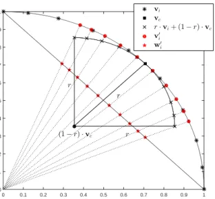
f1 0 0.1 0.2 0.3 0.4 0.5 0.6 0.7 0.8 0.9 1 f2 0 0.1 0.2 0.3 0.4 0.5 0.6 0.7 0.8 0.9 1 vi vc r·vi+ (1−r)·vc v′i w′i r r r (1−r)·vc
Fig. 1. A visualized illustration of the transformation procedure to generate weight/reference vectors inside a region specified by a central vectorvcand a radiusr. In this example, 10 uniformly distributed weight/reference vectors are generated inside a region in a bi-objective space specified byvc= (
√ 2 2 , √ 2 2 ) andr= 0.5.
with a radiusrto specify an ROI in the normalized objective space:
v0i= r·vi+ (1−r)·vc kr·vi+ (1−r)·vck
, (12)
where vi with i = 1, ..., N denotes the reference vectors
generated using (11), and v0i denotes the reference vectors inside the ROI specified by vc and r. To define a central
vector vc, the DM can first specify a vector uc according
to his/her preference and then normalize it into a unit vector usingvc =kuucck. As to the radiusr, any value ofr∈(0,1)is
applicable, where a smallerrindicates a relatively smaller ROI around the central vector, and a largerrwill result in a wider range of solutions around the central vector. It should be noted that, for better robustness, it is suggested to also include the extreme vectors (i.e. (1,0, ...,0), (0,1, ...,0), ..., (0,0, ...,1)) and the central vector vc into the preference based reference
vector set.
Similarly, to articulate DM’s preferences with weight vec-tors, the only step is to map the reference vectors generated by (12) onto a hyperplane using the following transformation:
w0i= v 0 i kv0 ik1 , (13)
where wi0 with i= 1, ..., N denotes the weight vectors that articulate DM’s preferences. The above geometrical transfor-mations to generate preference based weight/reference vectors is illustrated in Fig. 1.
It is worth noting that, if the DM has multiple (e.g., a number of K) ROIs, multiples preference based reference vector sets can also be obtained accordingly as follows:
v0k,i= rk·vk,i+ (1−rk)·vk,c krk·vk,i+ (1−rk)·vk,ck , (14) and w0k,i= v 0 k,i kv0 k,ik1 , (15)
where k = 1, ..., K. Therefore, given a number of K pref-erence central vectors, the size of a full prefpref-erence based reference vector set is K(N+ 1) +M, whereN is the size of the original vector set generated using (11) andM is the number of objectives.
To better understand how the proposed preference articu-lation approach works, we will show in the following some empirical results obtained on selected benchmark test prob-lems, i.e., DTLZ1 and DTLZ2 from the DTLZ test suite [64]. As shown by the results summarized in Fig. 2, a general observation is that all three algorithms work well with the proposed preference articulation approach. In addition, the following observations can also be made. First, as evidenced in Fig. 2(d) to Fig. 2(f), the proposed preference articulation approach is capable of dealing with multiple independent ROIs during one single run of the algorithm. Second, from Fig. 2(a) to Fig. 2(c), we can see that when the ROIs are overlapped, the proposed preference articulation approach also works well. Third, by tuning the preference radius r (e.g.,
r= 0.3 in Fig. 2(a) to Fig. 2(c) andr= 0.1 in Fig. 2(d) to Fig. 2(f)), the proposed preference articulation approach is able to adjust the size of the ROI covered by the weight/reference vectors. More empirical analyses of the proposed preference articulation method can be found in Supplementary Materials V, where comparisons are made with the recently proposed MOEA/D-PRE [61].
It is worth noting that although MOEA/D, NSGA-III and RVEA show very similar performance on the benchmark test problems using the proposed preference articulation approach, the results to be presented in Section V-C indicate that the performance of the three algorithms varies a lot on the seven-objective HEV controller model.
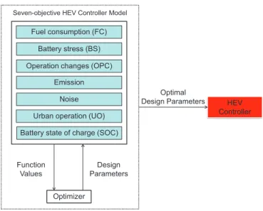
IV. SEVEN-OBJECTIVEHEV CONTROLLERMODEL
In hybrid electric vehicles (HEVs), the propulsion is pro-vided by a combination of internal combustion engine (ICE) and electric motor (EM). As a key element in the design of HEVs, the energy management controller (controller for short hereafter) plays an important role in guaranteeing peak performance of the hybrid power unit. As illustrated in Fig. 3, a general controller is used to determine in which condition the ICE and EM should be used [65]. In our case, since vehicle speed and torque are controlled by the driver or an externally given drive cycle, there is little freedom in the operation of the EM. Therefore, the controller basically controls the operation of the ICE only.
To be specific, HEV controller models are often designed on the basis of a small set of rules configured by a set of design parameters, i.e. the decision variables to the optimization objective(s). As listed in Supplementary Materials II, the proposed seven-objective HEV controller model is associated with a set of 11 design parameters that configure six basic control rules detailed in Supplementary Materials III.
0 0.2 f1 0.4 0.6 0.6 0.4 f2 0.2 0.2 0.1 0.4 0 0.3 0 0.6 0.5 f3 (a) MOEA/D (DTLZ1,r= 0.3) 0 0.2 f1 0.4 0.6 0.6 0.4 f2 0.2 0 0.1 0.2 0.3 0.4 0.5 0.6 0 f3 (b) NSGA-III (DTLZ1,r= 0.3) 0 0.2 f1 0.4 0.6 0.6 0.4 f2 0.2 0 0.1 0.2 0.4 0.5 0.6 0 0.3 f3 (c) RVEA (DTLZ1,r= 0.3) 0 0.2 0.4 f1 0.6 0.8 1 1 0.8 0.6 f2 0.4 0.2 0 0.2 0 0.4 0.6 0.8 1 f3 (d) MOEA/D (DTLZ2,r= 0.1) 0 0.2 0.4 f1 0.6 0.8 1 1 0.8 0.6 f2 0.4 0.2 0 0.2 0.4 0.6 0.8 1 0 f3 (e) NSGA-III (DTLZ2,r= 0.1) 0 0.2 0.4 f1 0.6 0.8 1 1 0.8 0.6 f2 0.4 0.2 0 0.2 0 0.4 0.6 0.8 1 f3 (f) RVEA (DTLZ2,r= 0.1)
Fig. 2. An example to assess the proposed preference articulation approach used by MOEA/D, NSGA-III and RVEA on three-objective DTLZ1 and DTLZ2. In this example, two central vectors, namely,(0.557,0.557,0.557)and(0.774,0.417,0.477)are given simultaneously to specify multiple DM’s preferences. Preference radiusr= 0.3andr= 0.1are applied for DTLZ1 and DTLZ2, respectively. To generate the preference based weight/reference set,H = 5is adopted for the simplex-lattice design in (10) to generate a number of21vectors around each central vector. The red dots, which are the preferred solutions approximated by each algorithm, are obtained with 100,000 fitness evaluations during one single run. The shape in blue in each figure denotes the true Pareto front. Internal Combustion Engine (ICE) Fuel Electric Motor/ Generator (EM) Battery Electricity Grid Wheels v(t) SOC(t) On/Off Operation Point Driver Request Speed HEV Controller Re-charging
Fig. 3. The sketch of the employed HEV architecture used for the study in this work. A conventional internal combustion engine (ICE), powered by fuel, charges a battery that drives an electric motor (EM) to propel the car. Before the start of the trip, the battery can also be charged from the electricity grid. During braking, the EM can act as a generator to re-charge the battery using kinetic energy. The amount of torque generated by the EM is defined by the driver (or in this case the driving cycle). The controller uses current speed, denoted asv(t), and current battery state-of-charge (SOC), denoted as SOC(t), as inputs and determines the operation of the ICE.
One of the most important objectives of a controller is to minimize the fuel consumption, and thus most existing work on optimal controller design has exclusively focused on this aspect [66]–[69]. To achieve the optimal control
TABLE I
SUMMARY OF THE SEVEN OPTIMIZATION OBJECTIVES IN THEHEV CONTROLLER MODEL.
Denotation Objective Name
FC Fuel consumption andCO2
BS Battery stress
OPC ICE operation changes
Emission ICE emissions
Noise Perceived ICE noise
UO Urban operation
SOC Average battery state of charge level
with a focus on fuel consumption, some traditional single-objective optimization methods such as dynamic programming (DP) [70]–[72] have been applied using a discretization of the decision variables in the control models and investigating all possible actions. As pointed out in [41], however, apart from fuel consumption, there are also other factors that may influence the overall performance of HEVs. For example, the driving experience, including noise, vibration, and harshness (NVH), is an important criterion for most customers while the battery lifetime is a major concern for manufacturers. Con-sidering that such additional factors may also have significant influence on the overall performance of HEVs, recently, an optimization model has been designed to simultaneously take seven objectives into consideration [41], where the objective names are summarized in Table I and detail definitions of the
objectives can be found in Supplementary Materials IV.
Fuel consumption (FC) Battery stress (BS) Operation changes (OPC)
Emission Noise Urban operation (UO) Battery state of charge (SOC)
Optimizer HEV Controller Design Parameters Optimal Design Parameters Function Values
Seven-objective HEV Controller Model
Fig. 4. An illustration of the architecture of the seven-objective HEV controller model and its relationship to the optimizer as well as the HEV controller. The seven-objective HEV controller model is connected to an op-timizer, e.g., a many-objective evolutionary algorithm. During the optimization process, the optimizer iteratively outputs candidate solutions of optimal design parameters to the seven-objective HEV controller model. As a feedback, the HEV controller model outputs the objective function values to the optimizer as fitness of the candidate solutions. Once the optimization is finished, the final optimal design parameters will serve as an input to the HEV controller to deploy the control rules.
To deploy the proposed controller, the seven-objective HEV controller model is applied to a plug-in serial HEV simulator with a battery capacity of 24.4 kWh, which is approximately 150 km of pure electric driving range. Instead of detailed ICE, EM, and battery models, we employ efficiency maps based on test-bench measurements in the form of look-up-tables. From a pre-specified speed profile, also known as driving cycle, the corresponding acceleration value to follow this speed profile is computed, and then a basic model of the HEV is used to determine the resulting information such as torque demand. With the information generated by the simulator, the function values of the seven optimization objectives can be calculated, which can be further used in the optimization procedure as fitness values. An illustration to the architecture of the seven-objective HEV controller model and its relationship to the optimizer as well as the HEV controller can be found in Fig. 4.
V. OPTIMIZATIONRESULTS
This section presents the optimization results obtained by MOEA/D, NSGA-III, and RVEA on the seven-objective HEV controller model. We first perform general optimization using the three algorithms as usually done in the literature and analyze the solutions. On the basis of these analyses, we incorporate DM’s preferences into the three algorithms to get corresponding candidate solutions, including the preference on minimizing objective of FC, and the preference on balancing the trade-off between the objectives of Noise and FOC.
A. General Optimization
Most MOEAs are designed for general optimization, i.e., for approximation of the whole Pareto fronts of MOPs as well as MaOPs with a limited number of candidate solutions. In this subsection, we apply MOEA/D, NSGA-III and RVEA to the optimization of the seven-objective HEV controller model without DM’s preferences.
To sample uniformly distributed reference vectors for such general optimization, the method introduced in Section III-A is adopted with settings ofH = 4, thus generating a number of 210 weight/reference vectors in total for each algorithm. Other parameter settings of the three algorithms are all the same as recommended in [25], [31] and [34], respectively.
To evaluate the quality of the solution sets obtained by each of the three algorithms, the hypervolume metric is applied as the performance indicator [38], [73]. LetPbe the approximate PF obtained by an MOEA, y∗ = (y1∗, ..., y∗M) be a reference point in the objective space. The HV value ofP (with respect to y∗) is the volume of the region which dominates point
y∗ and is dominated by all points in P. Here, we choose
[4,4,4,4,4,4,4] as the reference point y∗, where 4 is the worst possible value for all objectives that will be returned by the fitness functions (HEV simulator).
MOEA/D NSGA-III RVEA
Algorithm 4000 4500 5000 5500 6000 Hypervolume
Fig. 5. Statistical results for hypervolume values of the solutions obtained by the MOEA/D, NSGA-III and RVEA over 20 runs each.
A maximum number of 10000 fitness evaluations is used as the termination criterion for each algorithm in each run, and the statistical results of the hypervolume values obtained by each algorithm over 20 independent runs are summarized in Fig. 5. From the figure, we can see RVEA has achieved the largest mean value as well as the largest maximum value in HV among the three algorithms. On this optimization problem, MOEA/D performs slightly worse than NSGA-III.
While most benchmark tests of multi-/many-objective op-timization merely make statistical comparisons in terms of performance indicators of the solution sets, in real-world applications such as the optimization of a HEV controller, it is also of great interest to gain more insight into the problem by analyzing the trade-off relationships between the objectives. Therefore, in the following subsections, we will perform some analyses of the solutions obtained by all three algorithms,
based on which, the DM’s preferences will be incorporated into the optimizers.
B. Analyses of Solutions
In order to perform analyses of the solutions obtained by the three MOEAs, we use a configuration manually tuned by an experienced automotive engineer as the baseline solution3
(1,1,1,1,1,1,1) to normalize the objective values of the obtained solutions.
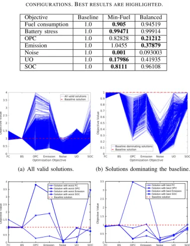
We first combine all solutions obtained by the three al-gorithms in 20 runs and remove the dominated solutions. As shown by the parallel coordinate plots in Fig. 6(a), the combined non-dominated solution set is well distributed around the baseline solution, showing highly diversified trade-offs between different objectives. In general, the majority of objective values are below the baseline for a large part of solutions, with a total 1086 solutions dominating the baseline solution, as shown in Fig. 6(b).
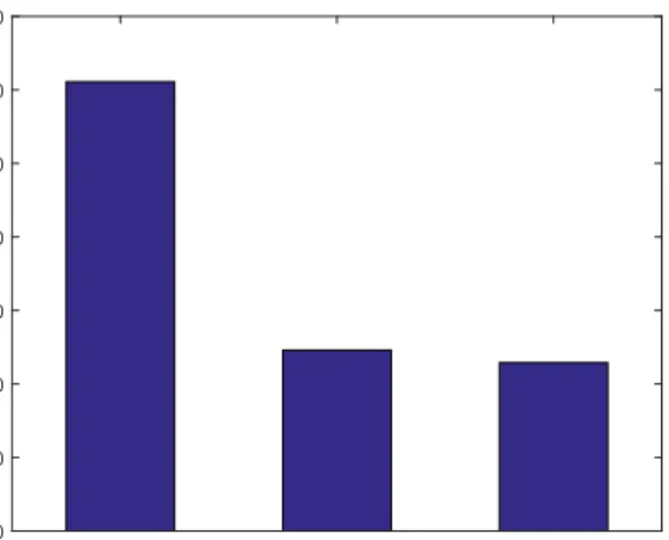
As shown in Fig. 7, MOEA/D has obtained 611 of the 1086 solutions that dominate the baseline solution, while NSGA-III and RVEA have obtained 246 and 229 solutions, respectively. This is an interesting observation as the ranking of the number of obtained non-dominated solutions is exactly opposite to the ranking of HV values as shown in Fig. 5. This is due to the fact that although MOEA/D achieves a large number of well-converged solutions, most of them are located in relatively small regions, leading to worse HV values. Empirical results to be presented in Section V-C confirm this observation.
Due to the conflicts between objectives such as FC, OPC, Emission and SOC, some solutions are significantly better than the baseline on these objectives, while others are significantly worse. For further investigations, the parallel coordinates of the extreme solutions that have the worst and best values on objectives of FC, OPC, Emission and SOC are plotted in Fig. 6(c) and Fig. 6(d), respectively. From these results, the following observations can be made.
First, as shown in both Fig. 6(c) and Fig. 6(d), OPC and Emission are highly consistent, as the solutions with the worst (as well as the best) OPC and Emission strongly overlap. These results indicate that the optima of OPC and Emission can very likely be achieved simultaneously. This is due to the fact that both objectives are very sensitive to the on/off changes of the ICE, which is consistent with the experience in HEV design. Second, Fig. 6(c) reveals that the objective of Noise is in conflict with the objective of SOC, where the solution with the best SOC has the worst Noise value. Such a relationship between Noise and SOC is not obvious as there is no direct physical connection between the two objectives. This relation-ship is definitely very useful in HEV design as a guideline to make trade-offs between the two objectives when tuning the design parameters.
Finally, as shown in Fig. 6(d), the solution with the best FC achieves around 10%improvement compared to the base-line solution. Such an improvement is significant because in
3In order to obtain the baseline solution, an experienced automotive
engineer had spent a large amount of time tuning and testing the configurations of the HEV simulator with the assistance of professional development tools.
practice, it is very likely that the improvement of FC is at the cost of other objectives such as Noise or SOC, while in the solutions obtained, most of the other objectives are also significantly improved in addition to the10%improvement on the objective of FC.
TABLE II
DESIGN PARAMETERS FOR THREE DIFFERENT CONTROLLER CONFIGURATIONS.
Parameter Baseline Min-Fuel Balanced
SOCmax(%) 70 34.494 35.314 SOCmin(%) 40 28.699 26.082 v1(km/h) 20 27.151 20.634 v2(km/h) 30 50.262 50.204 rev1(/m) 2500 2941 2907 torque1(N·m) 9.42 8.6269 8.2231 rev2(/m) 3500 3981 3070 torque2(N·m) 15.03 16.991 12.392 rev3(/m) 5500 4008 4946 torque3(N·m) 25.92 17.622 22.228 vof f (km/h) 20 39.057 20.298 TABLE III
OBJECTIVE VALUES FOR THREE DIFFERENT CONTROLLER CONFIGURATIONS. BEST RESULTS ARE HIGHLIGHTED.
Objective Baseline Min-Fuel Balanced
Fuel consumption 1.0 0.905 0.94519 Battery stress 1.0 0.99471 0.99914 OPC 1.0 0.82828 0.21212 Emission 1.0 1.0455 0.37879 Noise 1.0 0.001 0.093003 UO 1.0 0.17986 0.41935 SOC 1.0 0.8111 0.96108
(a) All valid solutions. (b) Solutions dominating the baseline.
FC BS OPC Emission Noise UO SOC Optimization Objective 0 0.5 1 1.5 2 2.5 3 3.5 4 Objective Value
Solution with worst FC Solution with worst OPC Solution with worst Emission Solution with worst SOC Baseline solution
(c) Solutions with the worst values on objectives of FC, OPC, Emission and SOC.
FC BS OPC Emission Noise UO SOC Optimization Objective 0 0.5 1 1.5 2 2.5 3 3.5 Objective Value
Solution with best FC Solution with best OPC Solution with best Emission Solution with best SOC Baseline solution
(d) Solutions with the best values on objectives of FC, OPC, Emission and SOC.
Fig. 6. Parallel coordinate plots of solutions obtained by MOEA/D, NSGA-III and RVEA in the final populations of 20 runs, in comparison with the baseline solution which is manually tuned by an experienced engineer.
In addition to the observations made above, we have also taken a more detailed look at two interesting solutions, the
Alogirthm
MOEA/D NSGA-III RVEA
Number of non-dominated solutions
0 100 200 300 400 500 600 700
Fig. 7. Number of non-dominated solutions obtained by MOEA/D, NSGA-III and RVEA, respectively among the combined non-dominated solution set achieved by the three algorithm in 20 runs.
solution with the best FC and the one with the best overall improvement (a plain sum of objective values), in comparison with the baseline solution. As summarized in Table II and Table III, the baseline solution is also given as a reference normalized to 1, and the solution with the best FC and the solution with the best overall improvement are listed in column “Min-Fuel” and column “Balanced”, respectively. While Table II presents the design parameters deployed by the controller of the HEV simulator, Table III presents the objective values output by the seven-objective HEV controller model.
0 1 2 3 4 5 Time (h) 0 20 40 60 80 100 120 Speed (km/h)
(a) Speed profile (drive cycle)
0 1 2 3 4 5 Time (h) 0 20 40 60 80 100
Fuel consumption (scaled) SOC (%) (b) Baseline configuration 0 1 2 3 4 5 Time (h) 0 20 40 60 80 100
Fuel consumption (scaled) SOC (%) (c) Min-Fuel configuration 0 1 2 3 4 5 Time (h) 0 20 40 60 80 100
Fuel consumption (scaled) SOC (%)
(d) Balanced configuration Fig. 8. The data of (instantaneous) fuel consumption (FC) and battery state-of-charge (SOC) with respect to the speed profile defined by the used driving cycle. The first figure shows the speed profile of the HEV, and the other three figures show the data generated by the HEV simulator which deploys controllers configured by different sets of design parameters (Baseline, Min-Fuel, Balanced), as defined in Table II.
For the solution with the best FC, it can be observed from column “Min-Fuel” in Table III that FC has been improved by approximately 10% in comparison with the baseline solution,
at the cost of a slight increase of Emission. For the solution with the best overall improvement, as presented in column “Balanced” in Table III, although FC is slightly higher than that of the solution with the best FC, the other objectives have substantially improved, by 43% averaged over all objectives, in comparison with the baseline solution, especially on Emission and Noise.
To further assess the quality of the representative solutions listed in Table II and Table III, we run the HEV simulator that deploys the control strategy using the design parameters listed in Table II and record the simulated data of FC and SOC generated during our project-specific drive cycle. As shown in Fig. 8, the data generated by the HEV simulator also shows observations that are consistent with our analyses above.
Based on the above analyses, the DM (HEV engineer) is particularly interested in further exploiting the potential improvement on one of the objectives such as FC and striking a better balance between other objectives. In the following, the above user preferences will be incorporated in the MOEAs to see if better solutions can be achieved.
C. Preference Articulation
As we previously discussed, general optimization is realistic for MOPs that have two or three objectives. For MaOPs having more than three objectives, however, approximation of the whole Pareto front in a very high dimensional space with a limited number of solutions becomes hardly possible. This challenge, however, has not been fully recognized. In the fol-lowing, we illustrate using the HEV controller design example why user preferences are important for solving practical many-objective optimization problems.
In the following experiments we show how to perform preference-driven optimization using MOEA/D, NSGA-III and RVEA with the proposed preference articulation approach. First, by using the solution with the best FC as a single preference central vector, we see if it is possible to further minimize FC. In addition, using solutions with the best SOC and best Noise as two simultaneous preference central vectors, we investigate the trade-off relationship between these two objectives.
1) Preference Articulation for Minimizing FC: To articulate
preference for minimizing the objective of fuel consumption (FC), we first specify the solution with the lowest FC value obtained in the general optimization as a preference central vector vc (refer to (12)), and then set the preference radius
as r = 0.1. It is worth noting that, although setting the minimization of one single objective (i.e., FC) as DM’s preference is conceptually different from traditional preference articulation methods, technically, the target is still realized by specifying an ROI using a preference central vector together with a preference radius. Consequently, the solutions obtained by MOEA/D, NSGA-III and RVEA are shown in Fig. 9, from which the following remarks can be made.
First, we can see from Fig. 9(a) that solutions obtained by MOEA/D distribute very closely to the preference central vector and thus lack a certain degree of diversity. This small degree of diversity in solutions might be caused by the neigh-borhood based steady-state reproduction mechanism adopted
FC BS OPC Emission Noise UO SOC Optimization Objective 0 0.5 1 1.5 2 2.5 3 3.5 4 Objective Value Obtained solutions Preference: Best FC
(a) Solutions obtained by MOEA/D.
FC BS OPC Emission Noise UO SOC
Optimization Objective 0 0.5 1 1.5 2 2.5 3 3.5 4 Objective Value Obtained solutions Preference: Best FC
(b) Solutions obtained by NSGA-III.
FC BS OPC Emission Noise UO SOC
Optimization Objective 0 0.5 1 1.5 2 2.5 3 3.5 4 Objective Value Obtained solutions Preference: Best FC
(c) Solutions obtained by RVEA.
Fig. 9. Parallel coordinate plots of solutions obtained by MOEA/D, NSGA-III, and RVEA using the solution with the best FC in general optimization as the preference central vector.
in MOEA/D. By contrast, NSGA-III and RVEA, which adopt a generational reproduction mechanism performed on the whole population, show significantly better population di-versity. Among the three algorithms, RVEA seems to have achieved the best balance between convergence and diversity. Second, NSGA-III is able to obtain a large number of very different solutions, most of which are away from the preference central vector. By contrast, RVEA and MOEA/D have obtained a smaller number of solutions that are close to or even better than the preferred solution on most objectives. These results imply that NSGA-III tends to generate more widely spread candidate solutions, but fails to stick to the preferences.
Third, as observed from Fig. 9(c), with a slightly higher FC, the HEV simulator is able to achieve a significantly better
FC BS OPC Emission Noise UO SOC
Optimization Objective 0 0.5 1 1.5 2 2.5 3 3.5 4 Objective Value Obtained solutions Preference: Noise Preference: SOC
(a) Solutions obtained by MOEA/D
FC BS OPC Emission Noise UO SOC
Optimization Objective 0 0.5 1 1.5 2 2.5 3 3.5 4 Objective Value Obtained solutions Preference: Noise Preference: SOC
(b) Solutions obtained by NSGA-III
FC BS OPC Emission Noise UO SOC
Optimization Objective 0 0.5 1 1.5 2 2.5 3 3.5 4 Objective Value Obtained solutions Preference: Noise Preference: SOC
(c) Solutions obtained by RVEA
Fig. 10. Parallel coordinate plots of solutions obtained by MOEA/D, NSGA-III, and RVEA using the solutions with the best Noise and the best SOC in general optimization together as the preference central vectors.
performance in OPC and Emission. This is due to the fact that turning on/off the ICE too frequently (to reduce FC) will cost not only additional operation changes (OPC), but also extra start-up operations of the ICE, both of which will produce more emissions. By contrast, if the controller adopts optimal design parameters which aim to reduce the number of OPC operations at a slight higher cost of FC, as shown in Fig. 9(c), the objective of Emission can be further improved.
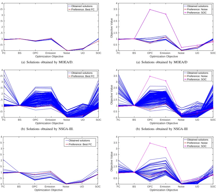
2) Preference Articulation for Trade-off between Noise and SOC: To articulate preference for trade-offs between Noise and SOC, the solutions with the best SOC and the best Noise obtained from the general optimization are used together as two preference central vectors vc (refer to (12) with the
preference radius being set to r = 0.1. From the results obtained by MOEA/D, NSGA-III and RVEA in Fig. 10, we
make the following observations.
First, the solutions obtained by all three algorithms (espe-cially MOEA/D) have a bias towards the solution with the best (lowest) Noise. Such an observation indicates that, in comparison with SOC, Noise is an objective that is relatively easier to optimize. This is due to the fact that, according to the definition of objective Noise in Supplementary Materials IV, keeping the ICE noise lower than the rolling noise will directly result in the minimum noise value, which can be achieved in HEV design by keeping the ICE in lower-power operation points. By contrast, keeping the SOC objective low will require to define a very narrow band of permissible SOC values, severely impairing other objectives and making it more difficult to achieve low SOC values in the optimization.
2.65 2.7 2.75 2.8 2.85 2.9 2.95 Time (h) 0 20 40 60 80 100 Noise (dB) Rolling noise ICE noise
Fig. 11. A comparison between ICE noise and rolling noise generated from wind/tires recorded by the simulator that deploys the controller configured by one of the solutions that trade off between Noise and SOC as shown in Fig. 10(c). Here only a representative part of the total drive cycle is shown.
Second, reducing Noise will consequently increase SOC, and vice versa, which indicates that the two objectives are in natural conflict and simultaneous optimization of both objectives are impossible. This knowledge is very helpful in HEV controller design as engineers can select a best trade-off solution from those obtained by the three algorithms, as shown in Fig. 10, instead of taking the time to fine tune design variables to simultaneously minimize both objectives. Here, we randomly select one trade-off solution obtained by RVEA in Fig. 10(c) to compare the ICE noise and the rolling noise recorded by the simulator. As shown in Fig. 11, by deploying the controller configured using the trade-off solution we select, the HEV controller manages to completely keep ICE noise below rolling noise, which satisfactorily meets the requirements of a low noise level in HEV design.
D. Discussions
From the above results, it is evident that the quality of the candidate solutions obtained using the three evolutionary many-objective optimization algorithms are significantly better than the baseline solution. Moreover, since there are multiple candidate solutions obtained during one run, it provides a better flexibility for decision making. As a result, the DM can perform further optimizations to obtain additional candidate
solutions or to investigate the relationships between different optimization objectives according to his/her preferences.
For MOEA/D, NSGA-III and RVEA, each of the three algo-rithms shows unique advantages over the other two when ap-plied to the optimization of the seven-objective HEV controller model, together. On the one hand, MOEA/D has exhibited the best convergence performance, although the solutions may be densely distributed in a narrow region, leading to a smaller degree of diversity. This implies that in practical applications, if the DM is more interested in convergence, MOEA/D is a good choice.
By contrast, NSGA-III shows the highest degree of diversity. No matter how the preference central vectors are set, the solutions obtained by NSGA-III are usually widely spread over the objective space, although most of the solutions are of relatively worse convergence in comparison with those obtained by the other two algorithms. Therefore, if the problem to be optimized has a relatively simple fitness landscape and the DM is interested in getting more information about PF, NSGA-III might be a good optimizer as it generates a wide distribution of the candidate solutions.
Finally, RVEA appears to have achieved the best balance between convergence and diversity. In general optimization, RVEA has achieved the highest HV value among the three algorithms. Meanwhile, in the preference based optimization, RVEA seems the most effective in achieving solutions pre-ferred by the DM, no matter whether a single or multiple preferences are given. Therefore, if the problem to be opti-mized has a relatively complicated fitness landscape and the DM has a clear target (i.e., preference) to be achieved, RVEA might be the best option.
VI. CONCLUSION
In this paper, we have applied three state-of-the-art MOEAs, namely, MOEA/D, NSGA-III and RVEA to the optimiza-tion of a seven-objective HEV controller model. We also have proposed a preference articulate method by means of weight/reference vectors to guide the three MOEAs to search for the solutions preferred by the decison-maker. The proposed preference articulation approach, which only requires a set of preference central vector(s) and a preference radius, can be easily used to specify ROIs in the objective space by gen-erating uniformly distributed weight/reference vectors inside them.
A number of experiments have been performed on the seven-objective HEV controller model. At first, we aimed to approximate the Pareto front using using uniformly distributed weights/vectors across the whole objective space. The obtained solutions were carefully analyzed to gain useful information between the objectives, based on which preferences were articulated in the MOEAs using the proposed preference articulation approach to further exploit the solution space according to DM’s preferences. Our experimental results have shown that, by applying the three MOEAs together with the preference articulation approach, the DM is not only able to obtain a deeper understanding of the relationships (i.e., conflicts and consistencies) between different optimization objectives, but also obtain more solutions in the ROIs.
From the results of the compared solutions on the real-world many-objective optimization problem, we can conclude that the state-of-the-art MOEAs studied in this work have shown very good performance yet slightly different search properties. These finding are instructive for practitioners who are interested in solving real-world many-objective problems using evolutionary algorithms. We hope this work will trigger more interests in the academia in addressing real-world hard problems and attract more attention from industry on the recent developments in evolutionary computation research.
ACKNOWLEDGMENTS
This work was supported in part by the Honda Research Institute Europe, and in part by the Joint Research Fund for Overseas Chinese, Hong Kong and Macao Scholars of the National Natural Science Foundation of China (Grant No. 61428302). The authors thank Mohammed Awada for support with the modeling of objectives and Kaname Narukawa for developing the initial many-objective optimization set-up.
REFERENCES
[1] R. T. Marler and J. S. Arora, “Survey of multi-objective optimization methods for engineering,”Structural and multidisciplinary optimization, vol. 26, no. 6, pp. 369–395, 2004.
[2] A. Ponsich, A. L. Jaimes, and C. A. C. Coello, “A survey on mul-tiobjective evolutionary algorithms for the solution of the portfolio optimization problem and other finance and economics applications,” IEEE Transactions on Evolutionary Computation, vol. 17, no. 3, pp. 321–344, 2013.
[3] P. M. Reed, D. Hadka, J. D. Herman, J. R. Kasprzyk, and J. B. Kollat, “Evolutionary multiobjective optimization in water resources: The past, present, and future,”Advances in water resources, vol. 51, pp. 438–456, 2013.
[4] K. Deb, A. Pratap, S. Agarwal, and T. Meyarivan, “A fast and elitist multiobjective genetic algorithm: NSGA-II,” IEEE Transactions on Evolutionary Computation, vol. 6, no. 2, pp. 182–197, 2002. [5] E. Zitzler, M. Laumanns, and L. Thiele, “SPEA2: improving the strength
Pareto evolutionary algorithm for multiobjective optimization,” inFifth Conference on Evolutionary Methods for Design, Optimization and Control with Applications to Industrial Problems, 2001, pp. 95–100. [6] D. W. Corne, N. R. Jerram, J. D. Knowles, and M. J. Oates,
“PESA-II: region-based selection in evolutionary multi-objective optimization,” in2001 Genetic and Evolutionary Computation Conference, 2001, pp. 283–290.
[7] A. Zhou, B.-Y. Qu, H. Li, S.-Z. Zhao, P. N. Suganthan, and Q. Zhang, “Multiobjective evolutionary algorithms: A survey of the state of the art,”Swarm and Evolutionary Computation, vol. 1, no. 1, pp. 32–49, 2011.
[8] K. Ikeda, H. Kita, and S. Kobayashi, “Failure of Pareto-based MOEAs: does non-dominated really mean near to optimal?” inProceedings of the IEEE Congress on Evolutionary Computation, 2001, pp. 957–962. [9] D. Brockhoff, T. Friedrich, N. Hebbinghaus, C. Klein, F. Neumann, and
E. Zitzler, “On the effects of adding objectives to plateau functions,” IEEE Transactions on Evolutionary Computation, vol. 13, no. 3, pp. 591–603, 2009.
[10] O. Sch¨utze, A. Lara, and C. A. C. Coello, “On the influence of the number of objectives on the hardness of a multiobjective optimization problem,” IEEE Transactions on Evolutionary Computation, vol. 15, no. 4, pp. 444–455, 2011.
[11] L. S. Batista, F. Campelo, F. G. Guimaraes, and J. A. Ram´ırez, “A com-parison of dominance criteria in many-objective optimization problems,” in Proceedings of the IEEE Congress on Evolutionary Computation, 2011, pp. 2359–2366.
[12] P. J. Fleming, R. C. Purshouse, and R. J. Lygoe, “Many-objective optimization: An engineering design perspective,” inProceedings of the International Conference on Evolutionary multi-criterion optimization. Springer, 2005, pp. 14–32.
[13] H. Ishibuchi, N. Tsukamoto, and Y. Nojima, “Evolutionary many-objective optimization: A short review,” inIEEE Congress on Evolu-tionary Computation, 2008, pp. 2419–2426.
[14] B. Li, J. Li, K. Tang, and X. Yao, “Many-objective evolutionary algorithms: A survey,”ACM Computing Surveys, vol. 48, no. 1, p. 13, 2015.
[15] X. Zou, Y. Chen, M. Liu, and L. Kang, “A new evolutionary algorithm for solving many-objective optimization problems,”IEEE Transactions on Systems, Man, and Cybernetics, Part B: Cybernetics, vol. 38, no. 5, pp. 1402–1412, 2008.
[16] M. Laumanns, L. Thiele, K. Deb, and E. Zitzler, “Combining con-vergence and diversity in evolutionary multiobjective optimization,” Evolutionary Computation, vol. 10, no. 3, pp. 263–282, 2002. [17] D. Hadka and P. Reed, “Borg: An auto-adaptive many-objective
evo-lutionary computing framework,” Evolutionary Computation, vol. 21, no. 2, pp. 231–259, 2013.
[18] G. Wang and H. Jiang, “Fuzzy-dominance and its application in evolu-tionary many objective optimization,” in2007 International Conference on Computational Intelligence and Security Workshops, 2007, pp. 195– 198.
[19] S. Yang, M. Li, X. Liu, and J. Zheng, “A grid-based evolutionary algorithm for many-objective optimization,”IEEE Transactions on Evo-lutionary Computation, vol. 17, no. 5, pp. 721–736, 2013.
[20] M. Li, S. Yang, and X. Liu, “Shift-based density estimation for pareto-based algorithms in many-objective optimization,” IEEE Transactions on Evolutionary Computation, vol. 18, no. 3, pp. 348–365, 2014. [21] X. Zhang, Y. Tian, and Y. Jin, “A knee point driven evolutionary
algorithm for many-objective optimization,”IEEE Transactions on Evo-lutionary Computation, vol. 19, no. 6, pp. 761–776, 2015.
[22] H. Wang, L. Jiao, and X. Yao, “Two arch2: An improved two-archive algorithm for many-objective optimization,”Evolutionary Computation, IEEE Transactions on, vol. 19, no. 4, pp. 524–541, Aug 2015. [23] Z. He and G. G. Yen, “Many-objective evolutionary algorithm: objective
space reduction and diversity improvement,” IEEE Transactions on Evolutionary Computation, vol. 20, no. 1, pp. 145–160, 2016. [24] M. Li, S. Yang, and X. Liu, “Pareto or non-pareto: Bi-criterion evolution
in multi-objective optimization,” IEEE Transactions on Evolutionary Computation, vol. 20, no. 5, pp. 645–665, 2016.
[25] Q. Zhang and H. Li, “MOEA/D: a multi-objective evolutionary algo-rithm based on decomposition,” IEEE Transactions on Evolutionary Computation, vol. 11, no. 6, pp. 712–731, 2007.
[26] H.-L. Liu, F. Gu, and Q. Zhang, “Decomposition of a multiobjective optimization problem into a number of simple multiobjective subprob-lems,”IEEE Transactions on Evolutionary Computation, vol. 18, no. 3, pp. 2450–455, 2014.
[27] Y. Yuan, H. Xu, B. Wang, B. Zhang, and X. Yao, “Balancing conver-gence and diversity in decomposition-based many-objective optimizers,” IEEE Transactions on Evolutionary Computation, accepted in 2015. [28] Y. Jin, M. Olhofer, and B. Sendhoff, “Dynamic weighted aggregation
for evolutionary multi-objective optimization: Why does it work and how?” in Proceedings of the Genetic and Evolutionary Computation Conference. ACM, 2001, pp. 1042–1049.
[29] T. Murata, H. Ishibuchi, and M. Gen, “Specification of genetic search directions in cellular multiobjective genetic algorithms,” inProceedings of the International Conference on Evolutionary Multi-Criterion Opti-mization, 2001, pp. 82–95.
[30] K. Li, Q. Zhang, and S. Kwong, “An evolutionary many-objective optimization algorithm based on dominance and decomposition,”IEEE Transactions on Evolutionary Computation, vol. 19, no. 5, pp. 694–716, 2015.
[31] K. Deb and H. Jain, “An evolutionary many-objective optimization algorithm using reference-point-based nondominated sorting approach, part I: solving problems with box constraints,”IEEE Transactions on Evolutionary Computation, vol. 18, no. 4, pp. 577–601, 2014. [32] R. Cheng, Y. Jin, K. Narukawa, and B. Sendhoff, “A multiobjective
evoltuionary algorithm using Gaussian process based inverse modeling,” IEEE Transactions on Evolutionary Computation, vol. 19, no. 6, pp. 838–856, 2015.
[33] R. Cheng, Y. Jin, and K. Narukawa, “Adaptive reference vector gener-ation for inverse model based evolutionary multiobjective optimizgener-ation with degenerate and disconnected pareto fronts,” inProceedings of the Evolutionary Multi-Criterion Optimization. Springer, 2015, pp. 127– 140.
[34] R. Cheng, Y. Jin, M. Olhofer, and B. Sendhoff, “A reference vector guided evolutionary algorithm for many-objective optimization,” IEEE Transactions on Evolutionary Computation, vol. 20, no. 5, pp. 773–791, 2016.
[35] N. Beume, B. Naujoks, and M. Emmerich, “SMS-EMOA: multiobjec-tive selection based on dominated hypervolume,”European Journal of Operational Research, vol. 181, no. 3, pp. 1653–1669, 2007.