Algorithms and Analysis for Multi-Category Classification

(1)

c

(2)

ALGORITHMS AND ANALYSIS FOR MULTI-CATEGORY CLASSIFICATION

BY

DAV ARTHUR ZIMAK B.S., Columbia University, 1998

DISSERTATION

Submitted in partial fulfillment of the requirements for the degree of Doctor of Philosophy in Computer Science

in the Graduate College of the

University of Illinois at Urbana-Champaign, 2006

(3)

Abstract

Classification problems in machine learning involve assigning labels to various kinds of output types, from single assignment binary and multi-class classification to more complex assignments such as category ranking, sequence identification, and structured-output classification. Traditionally, most machine learning algorithms and theory is developed for the binary setting. In this dissertation, we provide a framework to unify these problems. Through this framework, many algorithms and significant theoretic understanding developed in the binary domain is extended to more complex settings.

First, we introduce Constraint Classification, a learning framework that provides a unified view of complex-output problems. Within this framework, each complex-output label is viewed as a set of constraints, sufficient enough to capture the information needed to classify the example. Thus, prediction in the complex-output setting is reduced to determining which constraints, out of a potentially large set, hold for a given example—a task that can be accomplished by the repeated application of a single binary classifier to indicate whether or not each constraint holds. Using this insight, we provide a principled extension of binary learning algorithms, such as the support vector machine and the Perceptron algorithm to the complex-output domain. We also show that desirable theoretical and experimental properties of the algorithms are maintained in the new setting.

Second, we address the structured output problem directly. Structured output labels are col-lections of variables corresponding to a known structure, such as a tree, graph, or sequence that can bias or constrain the global output assignment. The traditional approach for learning struc-tured output classifiers, that decomposes a strucstruc-tured output into multiplelocalized labels to learn independently, is theoretically sub-optimal. In contrast, recent methods, such as constraint clas-sification, that learn functions to directly classify the global output can optimal performance. Surprisingly, in practice it is unclear which methods achieve state-of-the-art performance. In this

(4)

work, we study under what circumstances each method performs best. With enough time, training data, and representative power, the global approaches are better. However, we also show both theoretically and experimentally that learning a suite of local classifiers, even sub-optimal ones, can produce the best results under many real-world settings.

Third, we address an important algorithm in machine learning, the maximum margin classifier. Even with a conceptual understanding of how to extend maximum margin algorithms to more complex settings and performance guarantees of large margin classifiers, complex outputs render traditional approaches intractable in more complex settings. We introduce a new algorithm for learning maximum margin classifiers using coresets to find provably approximate solution to max-imum margin linear separating hyperplane. Then, using the constraint classification framework, this algorithm applies directly to all of the previously mentioned complex-output domains. In ad-dition, coresets motivate approximate algorithms for active learning and learning in the presence of outlier noise, where we give simple, elegant, and previously unknown proofs of their effectiveness.

(5)

(6)

Acknowledgments

The unconditional love and support of my family has given me the endurance to study for seven long years. Their immense confidence in me helped me to get through the rough spots and it gives me great pleasure to know that I have made them proud. Thank you Mom, Dad, Avi, Grandma, Grandpa, and O¨_{˘ mi.}

I am grateful to my advisor, Dan Roth, for his knowledge and vision. Not only has he steered me through my studies, but he has occasionally stepped on the gas for me as well. He allowed me the time to develop my own ideas and insights, and showed me how to transform them into real research. This dissertation would not exist without his wisdom and patience.

I am equally grateful to Sariel Har-Peled, who contributed to a large fraction of this work. With his help, I was able to understand concepts that appeared out of reach. He is the master of the counter example, and to acknowledge the many times he has changed the direction of my thought, I must acknowledge the corn.

Many people have contributed to this work in more ways than they know. Shivani Agarwal, Rodrigo de Salvo Braz, Yair Even-Zohar, Alex Klementiev, Xin Li, Marcia Mu˜noz, Nick Rizzolo, Mark Sammons, Kevin Small, Samarth Swarup, and Yuancheng Tu all helped me understand material that I could not grasp without them, including what is contained in this document.

Fabio Aiolli, Vasin Punyakanok, and Scott Wen-tau Yih have been particularly influential in my work. Through many sleepless nights working to make deadlines, I have gained true respect for each of them as researchers and as friends.

Finally, I would like to thank my dissertation committee, Gerald DeJong, Sariel Har-Peled, Lenny Pitt, and Dan Roth. I am very grateful for their comments, questions, suggestions, and perspective.

(7)

List of Tables

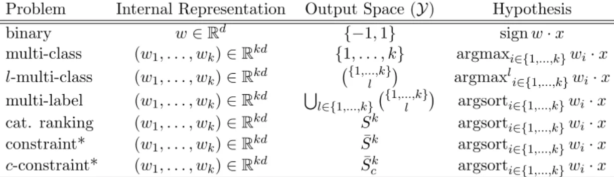
3.1 Summary of multi-categorical learning problems. . . 45

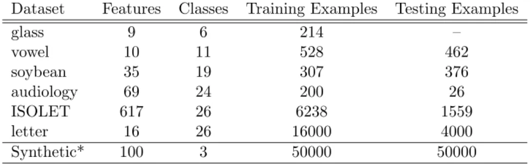
3.2 Summary of UCI datasets for multi-class classification. . . 58

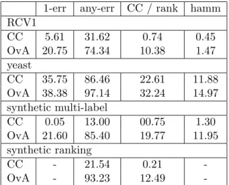
3.3 Experimental results of constraint classification on multi-label data. . . 62

4.1 Experimental results of multi-prototype margin perceptron on UCI datasets. . . 76

4.2 Effect of cooling parameter for multi-prototype margin perceptron. . . 76

4.3 Experimental results of semantic role labeling using multi-prototype margin percep-tron. . . 77

(11)

List of Figures

2.1 Perceptron-based learning of hidden Markov models. . . 26

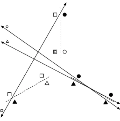
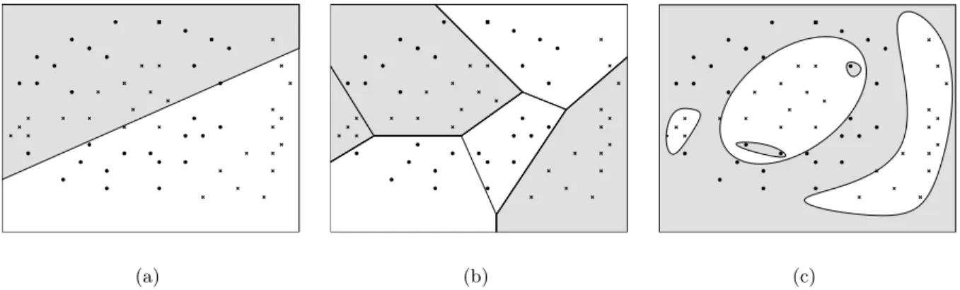
3.1 Learning of Voronoi diagrams. . . 38

3.2 Constraint classification meta-learning algorithm. . . 48

3.3 Robustness comparison between constraint classification and one-versus-all. . . 49

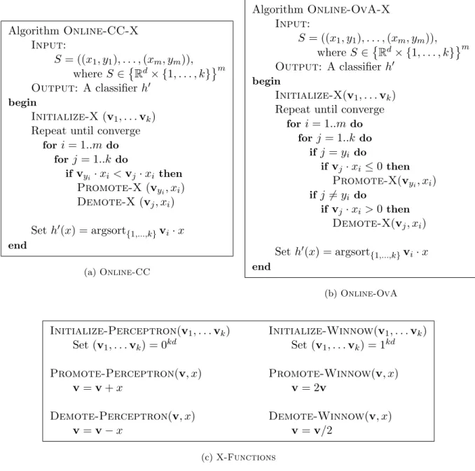
3.4 Online constraint classification for multi-class classification . . . 56

3.5 Experimental results of constraint classification on multi-class data. . . 58

3.6 Convergence graph of online constraint classification. . . 59

4.1 Decision regions of linear, multi-prototype, and kernel classifiers. . . 69

4.2 The multi-prototype margin perceptron algorithm. . . 74

4.3 Experimental results of semantic role labeling using multi-prototype margin percep-tron. . . 78

5.1 Inference based feedback learning algorithm. . . 84

5.2 Inference based training versus learning plus inference: synthetic data . . . 87

5.3 Inference based training versus learning plus inference: semantic-role labeling. . . 88

5.4 Inference based training versus learning plus inference: noun-phrase identification. . 89

5.5 Bound prediction for inference based training versus independent learning. . . 91

6.1 Maximum-margin learning via coresets. . . 98

6.2 Proof illustration for coreset bound. . . 100

6.3 Impossibility of zero-error approximation for active learning. . . 104

6.4 Active learning coreset algorithm. . . 106

(12)

Publication Note

This dissertation consists of enhanced versions of several previously published papers listed as follows.

Articles Incorporated into Thesis

- Constraint Classification: A Generalization of Multiclass Classification and Category Ranking with Sariel Har-Peled and Dan Roth

Journal of Artificial Intelligence Research (JAIR). In Submission. - Multi-Prototype Margin Perceptron

with Fabio Aiolli and Dan Roth Unpublished.

• Learning and Inference over Constrained Output with Vasin Punyakanok, Dan Roth, and Wen-tau Yih

Proc. of the International Joint Conference on Artificial Intelligence (IJCAI), 2005. Also appeared atLearning-05 The Learning Workshop, 2005.

First appeard atThe Conference on Advances in Neural Information Processing Systems (NIPS) Workshop on Learning Structured Output, 2004.

• Constraint Classification for Multiclass Classification and Ranking with Sariel Har-Peled and Dan Roth

The Conference on Advances in Neural Information Processing Systems (NIPS), 2002. • Constraint Classification: a New Approach to Multiclass Classification

with Sariel Har-Peled and Dan Roth

Proc. of the International Conference on Algorithmic Learning Theory (ALT), 2002.

Additional Articles

• Semantic Role Labeling via Generalized Inference over Classifiers Shared Task Paper with Vasin Punyakanok, Dan Roth, Wen-tau Yih and Y. Tu

Proc. of the Annual Conference on Computational Natural Language Learning (CoNLL), 2004 • Semantic Role Labeling via Integer Linear Programming Inference

with Vasin Punyakanok, Dan Roth, Wen-tau Yih

Proc. the International Conference on Computational Linguistics (COLING), 2004. • A Learning Approach to Shallow Parsing

with Marcia Munoz, Vasin Punyakanok and Dan Roth

The Joint SIGDAT Conference on Empirical Methods in Natural Language Processing and Very Large Corpora (EMNLP-VLC), 1999.

(13)

Chapter 1

Introduction

A multi-categorical classifier is a function that outputs one of many values from a potentially large discrete set, and is more general than a binary classifier that discriminates between only two values. They come in many flavors and are used in a wide range of applications. For example, in the multi-class setting, a discrimination over a small set of labels is desired, as in handwritten character recognition (Lee and Seung, 1997; Le Cun et al., 1989) and part-of-speech (POS) tagging (Brill, 1994; Even-Zohar and Roth, 2001). A second, more complex task is the multi-label problem where each example is labeled with a set of classes. In document (text) categorization, for example, a single document can be about both animals and survivalat the same time, just as a web page can be both an academic page and a homepage. Another related problem involves producing category rankings. For example, users can rate movies based on a scale ranging from 1 (hated) to 5 (loved) where there is an inherent relationship among the output classes. Thus, given a movie that a user loved, it is better to predict a rating of 4 than a rating of 2.

Furthermore, multi-category classification includes more complex problems, where the output conforms to a predefined structure. A closer look at the POS tagging task distinguishes it from the above problems. While it can be viewed as a multi-class problem by predicting one of about fifty POS tags for each word, it seems more natural to view it as a sequence prediction task, that assigns labels to each symbol in a variable length input. A POS tagger, for instance, should output a sequence of POS tags, one for each word in the input. Many other problems in natural language processing also conform to a complex structure, such as phrase identification and finding syntactic parse trees. Of course, problems of this type are all around us. In object identification, for example, when labeling the parts of a car, we know that there are usually a small number of wheels, a single window, a single steering wheel and various other parts — all with a fairly well defined relative orientation. Given an image, the set of assignments to all car parts should, perhaps, be viewed as a single classification that conforms to the structure defined by the concept of a car.

(14)

In one form or another, multi-category classification has been part of the study of artificial intelligence and machine learning from the beginning. Early work, focusing on logic (Newell et al., 1958), game playing (Shannon, 1950; Samuel, 1959), and neurological modeling (McCulloch and Pitts, 1943) all involve complex decision processes. Whether practical applications or true artificial intelligence is our goal, it is necessary to develop state-of-the-art learning algorithms for multi-categorical classification.

Despite the inherent interest in multi-categorical classification, almost all research in machine learning focuses on binary classification first. As a result, learning algorithms for binary classifica-tion are mature and well understood both theoretically and in practice. Probably approximately correct (PAC) bounds (Blumer et al., 1989; Valiant, 1984) show that generalization improves with simple hypotheses taken from a restricted set. Data-dependent bounds, such as those based on margin (Vapnik, 1998) show that well-separated data tends to be easier to classify. Perhaps, more importantly, a wide range of binary algorithms perform well in practice. It is becoming clear ex-actly how to design binary classifiers suitable for tasks that involve complex decision boundaries (say, with kernels (Boser, Guyon, and Vapnik, 1992)), tasks with various kinds of noise (Angluin and Laird, 1988; Sloan, 1988), and even tasks where not all of the examples are specified (Blum and Mitchell, 1998). Unfortunately, it is sometimes unclear how to extend these techniques to more complex classification tasks.

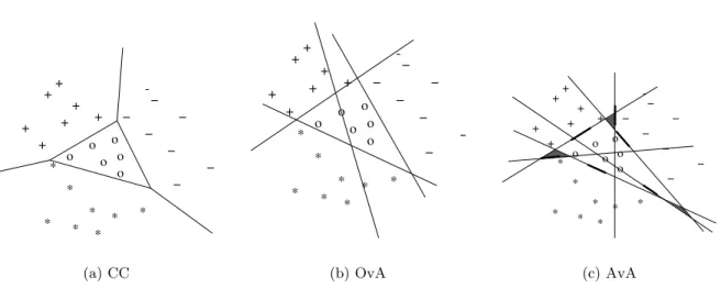
For many years, researchers studying binary classification often include a statement such as “This technique can easily be extended to the multi-class setting,” to emphasize the generality of the proposed approach. Unfortunately the actual construction of the multi-class classifier from the binary approach in the folklore is usually very crude. Indeed, it is common for authors to consider trivial extensions to multi-class classification. Perhaps the most widely used is the one-versus-all (OvA) approach, which makes use of an ensemble of standard binary classifiers to encode and train the output labels. The OvA scheme assumes that for each class there exists a single (simple) separation between that class and all the other classes. A more powerful approach, all-versus-all (AvA) (Hastie and Tibshirani, 1998), is a more expressive alternative that uses a binary classifier to distinguish each pair of classes ( n₂

classifiers in total). Other more subtle approaches exist as well. The error-correcting output coding scheme (ECOC) (Dietterich and Bakiri, 1995; Allwein, Schapire, and Singer, 2000) that generalizes OvA and AvA by using the idea that an ensemble of binary classifiers can be treated as an error-prone encoding of the true classes. Large

(15)

margin DAGs (Platt, Cristianini, and Shawe-Taylor, 2000) is a decision procedure that defines a flow over large margin binary classifiers. Similarly, when learning more complex classifiers over structured output (e.g. sequence prediction), a simple decomposition into constituent components yields a “cut-and-paste” approach where a single classifier predicts a value for each piece (Munoz et al., 1999) and the values are combined to form the ultimate prediction.

Unfortunately, as we will see in Chapter 3, many of the theoretical guarantees and practical performance made in the binary case do not hold when extended in this way. The difficulty lies in the fact that each of these methods learn a collection of independent classifiers and it is possible for each individual classifier to converge to an optimal classifier while the collection as a whole remains sub-optimal, if not poor. Two notable examples discussed at length in this thesis, are the perceptron algorithm and the support vector machine. The main theoretical justification for the use of the perceptron algorithm is the perceptron convergence theorem stating that the perceptron will learn any function it can represent. Unfortunately (as described in detail in Section 3.3.3), the most common in multi-categorical constructions do not preserve this property. Likewise, the support vector machine relies on the discovery of a large margin separation of the training data. The large margin approach requires not only a very specific definition of margin, but also a carefully tuned optimization procedure to maximize the minimum margin. Since the appropriate definition of margin implies a uniquely defined maximum-margin classifier, one must be very careful to to design a multi-category version of support vector machine that indeed optimizes the desired quantity.

However, despite all of the difficulties in developing general multi-categorical classifiers, the underlying concepts that produced efficient and effective algorithms in the binary case still exist with multi-categorical output. For example, despite the fact that multi-categorical classifiers are inherently more complicated than binary ones, it remains true that restricted hypothesis spaces produce better guarantees on future performance. Additionally, although the concept of binary margin does not directly apply to multi-categorical setting, the concept of learning functions that separate the input into tight clusters far away from the decision boundaries remains.

1.1

Thesis Statement

Multi-categorical tasks, such as multi-class, multi-label, categorical ranking, sequence labeling, and structured output tasks can be viewed under a single learning framework where the learning problems are mapped to a single instance of the binary task. As a

(16)

result, algorithms and analysis developed for learning binary classifiers can be applied to a wide range of multi-categorical tasks.

1.2

Contribution

The first contribution of this thesis is the introduction and development ofConstraint Classification in Chapter 3, a framework for learning multi-categorical classifiers. In a constraint-labeled example, the label consists of a set of pairwise preference relations among output classes. The goal of the constraint learning algorithm is simply to produce a function that accurately reflects the constraints specified in all examples. As a result, this framework captures many flavors of multi-categorical classification. A multi-class example simply prefers the correct class to all incorrect classes. A multi-label example prefers a set of classes to all classes not in that set. A ranking example orders the classes in a full order.

Although any function over pairwise preferences can be thought of as a constraint classifier, we focus on a simple linear representation and provide a learning algorithm that can naturally extend any binary learning algorithm. For multi-class classification, using Kesler’s construction (Nils-son, 1965), we construct a meta-algorithm for learning multi-class functions through the use of a single binary learning task. Through a simple extension of Kesler’s construction, we show that constraint-based learning algorithms easily generalize to these more complex tasks. Thus, con-straint classification extends existing learning algorithms for binary classification, however, unlike previous approaches, the extension is natural and often preserves desirable properties of algorithm from the binary case. When using a linear representation, we present distribution independent and margin-based generalization bounds as well as both empirical and theoretical evidence showing how constraint classification benefits over existing methods of multi-class classification.

As a result of our study of constraint classification, it became clear that learning in complex output domains is simplified through the very simple idea of viewing the label as a set of preferences, dictating a set of constraints that the classifier must obey. The same observation has lead to recent developments in structured classification (Collins, 2002; Taskar, Guestrin, and Koller, 2004). Specifically, by maintaining the constraint dictating that the correctglobal assignment must achieve a higher functional score from the classifier, various binary learning algorithms were applied to the structured domain. These include the perceptron algorithm (Collins, 2002), a maximum-margin based algorithm (Taskar, Guestrin, and Koller, 2004) and the support vector machine for

(17)

structured classification (Tsochantaridis et al., 2004; Altun, Tsochantaridis, and Hofmann, 2003). Indeed, viewing these new algorithms as instances of constraint classification provides additional justification for their use and a unifying view of all of these algorithms in the structured output domain.

Like constraint classification, these global techniques are provably sound and optimize an ob-jective directly related to the actual problem at hand. However, there is an inherent obstacle – complex output spaces inevitably increase the complexity of the underlying learning problem. For example, it may require more examples to learn a million-way discriminant function than a 2-way function. While this general assertion may seem intuitive, it becomes relevant in the structured output setting because of the exponential number of output labels imposed by these problems (for example there are possible kn labels in a length n k-way task). Thus, it may be the case that while learning globally is asymptotically optimal, learning simple classifiers at the local level may be superior when the total number of examples are limited.

In Chapter 5, we study the tradeoff between learning a functionally accurate, but complicated global classifier versus learning a collection of simple, but functionally inaccurate local classifiers for structured output problems. Specifically, we study learning structured output in a discriminative framework where values of the output variables are estimated by local classifiers. In this framework, complex dependencies among the output variables are captured by constraints and dictate which global labels can be inferred. We compare two strategies, learning independent classifiers (L+I) and inference based training (IBT). The L+I approach learns a set of independent classifiers to classify each output symbol separately (akin to the OvA approach), while IBT learns with respect to a global feedback so that the final classifier more accurately reflects the global assignment as a whole. We provide an experimental and theoretical analysis of the behavior of two approaches under various conditions. It turns out that using IBT is superior when the local classifiers are difficult to learn. However, it may require many examples before achieving high performance. On the other hand, when the number of examples are limited, as can be the case with many structured output tasks, L+I training can outperform IBT training.

Finally, we address efficiency concerns for an important instance of the multi-category problem – large margin learning. In Chapter 6 introduce coresets for maximum margin linear separating hyperplanes. Using coresets, we show an efficient algorithm for finding a (1−)-approximate max-imum margin separation for binary data. This concept is very general and motivates approximate

(18)

algorithms for learning in structured output domain and in active learning. Finally, we extend the idea to learning in the presence of noise, where we give the first polynomial time algorithm for learning an approximate separations.

(19)

Chapter 2

Preliminaries

This chapter reviews preliminary work that we build on and use in throughout the thesis. First, I describe the basic view of learning classifiers used in the following chapters.

2.1

Learning Classifiers

This thesis is entirely about learning classification functions. A classifier is a function c :X → Y from an instance space X to an output space (or label set) Y. When learning, we look for a hypothesis h : X → Y from a larger set of functions, H, the hypothesis space — in this thesis, we often return to a linear setting, where X = Rd and H is a collection of linear functions in Rd. A multi-categorical classifier is a classifier where the output space is a discrete set and the

classifier produces one of the set. In Chapters 3 and 4 we consider problems over a small output set, such as the multi-class (Y ={1, . . . , k}), multi-label (Y = S

l∈{1,...,k}

{1,...,k}

l

), and category ranking (Y = Sk, where Sk is the set of permutations over {1, . . . , k}) tasks. In Chapter 5, we consider a more general problem, the structured output problem, when the labels are more complex — in particular, we consider the case when the labels are sequences adhering to an arbitrary set of constraints, C ⊆ Y, (Y={y∈ {1, . . . , k}+|y /∈ C}).

The goal of learning a classifier function is to find a function from H that minimizes the error on future, unseen examples. More precisely, learning is the process of finding the function that minimizesrisk,

R(h) = Z

L(y, h(x))dDX ×Y,

where a loss function,L(y,y0), measures the difference betweeny and y0 and DX ×Y is the

prob-ability of observing example (x,y). The choice of loss function defines they the type of learning that is performed. In this dissertation, we consider only classification problems, where the loss can

(20)

be defined in various ways. The most straightforward is thezero-one loss, L01(y,y0) =    0 ify=y0 1 ify6=y0, (2.1)

where no loss is accrued if y=y0.

Other types of loss may arise when dealing with various multi-categorical problems. For exam-ple, one may wish to consider the number of incorrect tokens in a sequential prediction.

The empirical risk minimization (ERM) principle sates that rather than minimize the true loss, which can be difficult (or often impossible) to compute because the joint distributionDX ×Y

is unknown, the learning algorithm minimizes theempirical risk, Remp(h) = 1 m m X i=1 L(yi, h(xi)),

over a set of training examples,S = ((x1,y1), . . . ,(xm,ym)) drawni.i.d. from DX ×Y. As a result

of the ERM principle, the learned hypothesis will not necessarily be the best with respect to the true risk.

Sometimes, we refer to the zero-one loss above, as error. For convenience, we use various forms of error throughout the dissertation.

Definition 2.1.1 (Error) Given two labels, y,y0 ∈ Y, the error is the zero-one loss, E(y,y0) = L01(y,y0). Given an example, (x,y) and a hypothesis h ∈ H, the error is E(x,y, h) =E(h(x),y).

Given a sample S = ((x1,y1), . . . ,(xm,ym)), the error on the sample of a hypothesis h ∈ H is

E(S, h) = _m1 Pm

i=1E(xi,yi, h). Finally, given a distribution of examples DX ×Y, the expected error

of a hypothesis isED(h) =E(x,y)∼DE(x,y, h).

2.2

The Discriminant Approach to Learning Classifiers

Here, we describe the general discriminant model of learning to highlight how it can be used in the multi-categorical domain. Given input and output space,X and Y respectively, adiscriminant function is a real valued function,

(21)

used for classification. We refer to g(x,y) as the score of y given input x. Then, a discriminant classifier is a classifierh:X → Y of the form,

h(x) = argmax y∈Y

g(x,y). (2.2)

Any function such that

g(x,y)> g(x,y0) y0 ∈ Y \y,

scores the “correct” output label higher than any other and classifies example x correctly (i.e. E(x,y, h) = 0). Thus, we can think of a discriminant classifier as composed of two parts – a discriminant function, g(x,y), and inference procedure, argmax_y_∈Y, to find the highest scoring output in Equation 2.2.

An important specialization of this approach is obtained by using a joint feature space, Z as an intermediate representation and a feature map

Φ :X × Y → Z

to map an example and label (x,y) to a joint space. Then, the learning problem becomes to learn a discriminant functionf :Z →R. A further specialization is to represent the discriminant function

as a linear function in the joint space,f(x,y) =w·Φ(x,y). Representing features as a joint map has proved useful for describing structured classification tasks (see below and (Collins, 2002; Altun, Tsochantaridis, and Hofmann, 2003; Tsochantaridis et al., 2004)).

2.2.1 Examples

The joint feature map is a very general representation for classifiers and encapsulates many rep-resentations of interest from probabilistic and generative models to models designed solely for discrimination such as statistical linear classifiers and regression models. Clearly each piece must be carefully defined in order to obtain effective representations and learning algorithms.

Example 2.2.1 (Na¨ıve Bayes (NB)) The NB classifier is derived from a generative model. It models the probability of the output y∈ Y given the input x= (x1, . . . , xd)∈X˜d=X, as P(y|x),

P(y|x) = P(x|y)P(y) P(x) =

Qd

i=1P(xi|y)P(y)

(22)

by making the very strong conditional independence assumption that the variables,xi, are

indepen-dent given the output (P(xi, xj|y) =P(xi|y)P(xj|y) for all i6=j).

Used as a classifier, h(x) = argmax y∈Y P(y|x) = argmax y∈Y d Y i=1 P(xi|y)P(y) = argmax y∈Y d X i=1 logP(xi|y) + logP(y) = argmax y∈Y d X i=1 wxi,y+wy. (2.3)

Thus, the above expression is simply a linear sum weights, wxi,y= logP(xi|y) andwy= logP(y). This can be carefully rewritten as a single inner product over an appropriately defined feature vector. Specifically, letting weightswx,˜˜y= logP(˜x|˜y) (andwy˜ = logP(˜y)), and indicator functions

φx,˜y˜(x,y, i) = 1 when x˜=xi and 0 otherwise (and φy˜(y) = 1 when y˜ =y and 0 otherwise), then

the above can be rewritten as

h(x) = argmax y∈Y X ˜ x∈X˜,y˜∈Y wx,˜˜y d X i=1 φx,˜y˜(x,y, i) + X ˜ y∈Y wy˜φy˜(y) = argmax y∈Y X ˜ x∈X˜,y˜∈Y wx,˜˜yφx,˜y˜(x,y) + X ˜ y∈Y wy˜φy˜(y) = argmax y∈Y X c∈C wcφc(x,y) = argmax y∈Y w·Φ(x,y), (2.4)

where we have consolidated terms by defining φ˜x,y˜(x,y) =Px,˜y˜(x,y, i) to accumulate how many

times to add wx,˜˜y to the expression. By indexing all (˜x,y˜) pairs and y˜ assignments using c = 1, . . . , C, we write the final calculation as a linear function over joint feature space.

Example 2.2.2 (Hidden Markov Models (HMMs)) A HMM is a generative model that de-termines the likelihood of sequential output y = (y1, . . . , yd) ∈ Y˜∗ = Y given sequential input,

x = (x1, . . . , xd) ∈ X˜∗ = X, where Y and X are compositions of a number of component-wise

outputs, Y˜ and X˜, respectively. For a detailed description of the generative model, see (Rabiner, 1989; Bengio, 1999), here we will focus on linearizing the representation as in (Roth, 1999; Collins,

(23)

2002). In HMM, the input is sequential and it respects dependencies only between adjacent vari-ables — first, that the the variable at state t, xt, is conditionally independent of all previous states

1, . . . , t1 given the value of the variable at the previous state, t−1,

P(xt|xt−1, xt−2, . . . , x1) =P(xt|xt−1),

and second, that output variables at state t, yt, depend only on the input variable xt,

P(yt|yd, . . . , yt+1, yt−1, . . . , y1, xd, . . . , x1) =P(yt|xt).

Then, the probability of assignment (x,y) is defined as,

P(y,x) =

d

Y

t=1

P(yt|xt)P(xt|xt−1),

and is used to classify new examples by finding the maximum likelihood assignment of the output, given the input

h(x) = argmax y∈Y P(y|x) = argmax y∈Y d Y t=1 P(yt|xt)P(xt|xt−1) = argmax y∈Y d X t=1 logP(yt|xt) + logP(xt|xt−1) = argmax y∈Y d X t=1 wyt,xtφyt,xt(x,y, t) + d X t=1 wxt,xt−1φxt,xt−1(x,y, t) = argmax y∈Y X ˜ y∈Y˜,x˜∈X˜ wy,˜˜x d X t=1 φy,˜˜x(x,y, t) + X ˜ x,x˜0_∈_X˜ wx,˜x˜0 d X t=1 φx,˜x˜0(x,y, t) = argmax y∈Y X ˜ y∈Y˜,x˜∈X˜ wy,˜˜xφy,˜x˜(x,y) + X ˜ x,x˜0_∈_X˜ wx,˜˜x0φ_x,_˜_x_˜0(x,y) = argmax y∈Y X c∈C wcφc(x,y) =w·Φ(x,y) (2.5)

where I have used the notational convention that P(x1|x0) = P(x1), since x0 does not exist. As

in (Collins, 2002) and the previous example for Na¨ıve Bayes, we introduce

Φ(x,y) = (φ1(x,y), . . . , φC(x,y)) as to map the input/output pair (x,y) to a joint feature space.

(24)

log-probabilities should be added to the overall calculation. First, each log-probability is written as a weight, for example wy,x = logP(y|x). There is a different weight for each possible assignment to

every (y, x) pair and every (x, x0) pair. Then, to indicate which weights should be used in the log-probability calculation, we set φy,x(x,y, t) = 1if yt=y and xt =x and 0 otherwise. The number

of times wy,x is used is simply φy,x(x,y) =

P

t=1...dφy,x(x,y, t). After an appropriate indexing of

all possible assignments, c = 1, . . . , C to all (y, x) and (x, x0) pairs, Φ(x,y) represents the joint feature map, andw·Φ(x,y) represents the log-probability.

Example 2.2.3 (Multi-class) In multi-class classification, Y = {1, . . . , k}, and the multi-class classifier simply chooses the highest scoring output class. Consider the case where each class y ∈ {1, . . . , k} is represented with a linear function over a common feature space,Φ :X →_Rd_{, as with}

multi-class versions of perceptron, SVM, and CC in Chapter 3. Then, the hypothesis choosing the class with the highest score can be written in the general discriminant model,

argmax y∈{1,...,k} wy·Φ(x) = argmax y∈{1,...,k} (w1, . . . ,wk)·(Φ1(x, y), . . . ,Φk(x, y)) = argmax y∈{1,...,k} w·Φ(x, y),

where w= (w1, . . . ,wk) is the concatenation of the class weight vectors and

Φ(x, y) = (Φ1(x, y), . . .Φk(x, y))is the concatenation of special vectors Φi(x, y)∈Rd where

Φi(x, y) = Φ(x) when i=y and Φi(x, y) =0d (the zero vector of degree d) wheni6=y. It is easy

to see that the above equation simply rewrites the decision rule. See Chapter 3 for a very detailed description of this case.

2.2.2 Learning Discriminant Classifiers

In the rest of this Chapter (and the dissertation), many approaches are reviewed for learning multi-categorical classifiers. Here, we set up an important distinction between two general approaches – local and global learning.

Local Learning

In almost all cases, the traditional approach for learning in this model, has been to use some kind of (local) decomposition. For example, a binary (Y ={−1,1}) classifier in the above model must ensure thatf(Φ(x, y))> f(Φ(x,−y)), but is often reduced to a single functionfbin(Φ(x, y))>0.

(25)

(even in the linear case) ends with binary classification.

In practice, learning a multi-class (Y = {1, . . . , k}) classifier is often reduced to a set of in-dependent classifiers. As mentioned already, one way is the OvA approach, where each classifier tries to discriminate between a single class and the rest by restricting Φ :X → Z and defining a set of functions {fi}ki=1 such that fj(Φ(x))> 0 if and only ifj =y. Then f(Φ(x, y)) =fy(Φ(x))

and h(x) = argmaxy∈{1,...,k}fy(Φ(x)). An alternate method, constraint classification, is proposed

in Chapter 3 and uses the discriminant model directly to guarantee thatfy(Φ(x))> fy0(Φ(x)), for

all y0 ∈ {1, . . . , k} \y.

Similarly, a common decomposition for sequences uses a set of functions corresponding to the alphabet of the sequence. Specifically, ifY ={1, . . . , k}+is the set of all sequences over the alphabet {1, . . . , k}, then once could decompose the classifier into a set of scoring functions,{fy}ky=1. In this

case, given an example, (x,y) the score of the sequence is the sum of all of the disjoint functions over the sequence,

f(Φ(x,y)) =

|y|

X

i=1

fyi(Φi(x,y))

where Φi(x,y) is a transformation of (x,y) relative to the “position” in the sequence and are often

defined by position, region, or the entire sequence. Then, the learning problem can be decomposed into learning each function, fy separately such that fy(Φi(x,y)) > 0 if and only if yi = y in

example (x,y). Such approaches are often very successful in practice (Punyakanok and Roth, 2001; McCallum, Freitag, and Pereira, 2000; Punyakanok et al., 2004).

Global Learning

In light of the general discriminant framework, the learning problem becomes very straightforward. Simply find a functionf, such that for every example (x,y)∈S,

f(Φ(x,y))> f(Φ(x,y0)) ∀ y0∈ Y \y.

For the linear case, when f(Φ(x,y)) = w·Φ(x,y), a very nice geometric interpretation exists. Specifically, since we wish to learn a classifier represented byw∈Rd,

(26)

Conceptually, we can form Φ(x,y,y0) = Φ(x, yy)−Φ(x,y0) as a new “pseudo”-example inRd and view ˜S = n Φ(x,y,y0) (x,y)∈S, y

0₆₌_yo _{as a new “pseudo”-example set. Then, any function} wsuch that

w·˜x>0, ∀ ˜x∈S,˜

can be used as a classifier. This construction, a generalization of Kesler’s construction (see Sec-tions 2.3.4 and 3.3.1), provides a very direct learning problem for any joint feature space.

Comments

Both approaches can be applied to a wide range of multi-categorical output problems resulting from the general form of the feature map, Φ(x,y). Traditionally, most learning approaches are based on local decompositions. Until recently (Har-Peled, Roth, and Zimak, 2003; Collins, 2002; Crammer and Singer, 2000a), it was unclear that direct global learning approaches could be used even for the basic multi-class setting. in Chapter 3, we see that it is possible to effectively model various interesting learning problems over a small output space in a unified setting. As part of this work, we present the multi-class, multi-label and ranking in this framework and provide theoretical and experimental evidence suggesting that thisglobal approach is superior.

In addition, recently algorithms have been presented for sequential classification and structured output classification based on the general discriminant approach . In these works, various learning algorithms were applied to problems in this domain — the running theme through them was to model the structured output via a feature map, Φ(x,y) and learn with the Perceptron (Collins, 2002), SVM (Tsochantaridis et al., 2004; Altun, Tsochantaridis, and Hofmann, 2003) or a general maximum margin approach (Taskar, Guestrin, and Koller, 2004) a function fstruct(Φ(x,y)) =

w·Φ(x,y) to satisfy Equation 2.2.

However, as we see in Chapter 5, these new global approaches do not always yield state-of-the-art performance. We explore under what conditions each method is expected to perform best. Specifically,if the decomposition is accurate, then one might expect the local approach to perform better. However, since long sequences and large output structures can increase the difficulty of the overall task, is it possible that local approaches can outperform global ones even when the local decomposition is less than ideal.

(27)

2.3

Multi-class Classification

Beyond learning binary classifiers, multi-class classification is perhaps the most widely studied learning problem. A multi-class classifier outputs one of a (relatively) small, and enumerable set Y ∈ {1, . . . , k}. This section reviews some of the most commonly used approaches to multi-class classification.

2.3.1 One-versus-All (OvA) Decomposition

The most straightforward approach is to make the one-versus-all (OvA) assumption that each class can be separated from the rest using a binary classifier. Learning the multi-class function is decomposed to learning k independent binary classifiers, one corresponding to each class, where example (x, y) is considered positive for classifiery and negative for all others.

Specifically, given a set of training examples, S, for each classi∈ {1, . . . , k}, define a projected example set Si, Si = n x,[y=i]−1/1) (x, y)∈S o ,

where [a=b]−1/1 is 1 if a=b and −1 otherwise. Each example from the projected example set is

a projection of an example in the original example set,S.

Then, a single function, fi = L(Si,H), is learned for each class i ∈ {1, . . . , k}. Here I am

assuming some common and fixed hypothesis class for each learning sub-task.

The OvA scheme assumes that for each class there exists a single (simple) separation between that class and all the other classes. Unfortunately, the strong separability assumption of each classifier can yield the true (global) function unlearnable. See Section 3.3.3 for a comprehensive comparison between OvA and Constraint Classification for the linear case.

2.3.2 All-versus-All (AvA) Decomposition

A more powerful approach,all-versus-all (AvA), is a more expressive alternative that assumes the existence of a separation between every pair of classes. Similarly to the OvA setting, we define a set of projected example sets,

Sij = n x,[y=i]−1/1) (x, y)∈S, y∈ {i, j} o ,

(28)

where an example is projected intoSij only if it is from classior classj. Then, as before, we learn

a set of functions, fij =L(Sij,H) for all i6=j. here however, each function represents the decision

boundary between each pair of classes.

AvA is, in some sense, more expressive than OvA since it tries to capture the local interaction between every pair of classes using a greater number of functions — thus it reduces the multi-class problem to smaller and easier problems than the OvA approach. However, it is at the cost of increased complexity ( n₂ classifiers are required). Additionally, non-trivial decision procedures may be required for classification since the output of the many binary classifiers need not be coherent (an example may be predicted to be in class 1 over class 2, class 2 over class 3, and class 3 over class 1). Rather than assign random labels when a disagreement occurs, one can choose the class that is predicted by the maximum number of classifiers (Friedman, 1996), or use the output of the classifiers if it is know that they are probability estimates (Hastie and Tibshirani, 1998). However, taking a two staged approach can produces unintended consequences since it is impossible to knowhow the binary classifiers will err and if the second stage will correct the first stage errors.

2.3.3 Error-Correcting Output Coding (ECOC)

A more recent generalization of the last two approaches uses error correcting output coding(ECOC) to decompose the multi-class problem so that each binary classifier partitions the set of classes into arbitrary subsets and uses ECOC to fix the errors induced from difficult to learn partitions (Diet-terich and Bakiri, 1995; Allwein, Schapire, and Singer, 2000). The Basic ECOC model defines a coding matrix E ∈ {−1,1}k×L_{, to encode each class. The codeword matrix can be viewed in two}

ways: the rows provide an encoding of each of the k output classes and the columns provide L dichotomies of the data. Then, as with OvA and AvA, we define a set of projected examples sets,

Sl= n x, eyl (x, y)∈S o ,

one for each dichotomy, l = 1, . . . , L defined in the code matrix. Then a set of functions, fl =

L(Sl,H), is learned for each projected example set Sl. Finally, the ECOC classifier uses

error-correcting output coding to classify the new data, h(x) = argmin

y∈{1,...,k}

(29)

where ek− is the k-th row in E (i.e. the codeword for class k), f(x) = (f1(x), . . . , fL(x)), and

dH(u, v) is the hamming distance between two vectors u, v ∈ {−1,1}L. Using alternate code

matrices (E ∈ {−1,0,1}), it is easy to see that ECOC generalizes OvA and AvA.

2.3.4 Kesler’s Construction for Multi-class Classification

Kesler’s construction for multi-class classification was first introduced by Nilsson in 1965 (Nilsson, 1965, 75–77) and more recently in the popular book by Duda and Hart (Duda and Hart, 1973). It is a very powerful tool for extending learning algorithms for binary classifiers to the multi-class setting. Unfortunately it has long been ignored in many recent works on multi-class classification.

Given a set of multi-class examples, S = ((x1, y1), . . . ,(xm, ym)), where each

(xi, yi)∈Rd× {1, . . . , k}, we look for a linear classifier of the form,

h(x) = argmax

k

wk·x,

where wk ∈ Rd. Rather than learn a linear function directly for each of the wk, based on a

decomposition method, Kesler observed that by transforming S to a alternate set, P(S), a single linear function could be learned directly overP(S) and used inh(x).

Definition 2.3.1 (Chunk) A vector v = (v1, . . . , vkd) ∈ Rkd = Rd× · · · ×Rd, is broken into k

chunks (v1, . . . ,vk) where the i-th chunk, vi= (v(i−1)(d+1), . . . , vid).

Definition 2.3.2 (Expansion) Let Vec(x, i) be a vector x ∈ _Rd _{embedded in} _kd _dimensions,

by writing the coordinates of x in the i-th chunk of a vector in Rk(d+1). Denote by 0l the zero

vector of lengthl. Then Vec(x, i) can be written as the concatenation of three vectors, Vec(x, i) = (0(i−1)d, x,0(k−i)d)∈_Rkd_{. Finally, Vec(}_{x, i, j}_{) = Vec(}_{x, i}₎₋_Vec(_{x, j}_{), is the embedding of}_x _{in the}

i-th chunk and −x in thej-th chunk of a vector in Rkd.

Then,

P(S) ={Vec(x, y, j) :∀j6=y,∀(x, y)∈S}.

As a result, one can learn a linear classifier for the multi-class case simply by learning a binary (actually a unary) classifier w ∈ _Rkd _over _P₍_S_{). Specifically, any} _w _{= (}_w1_{, . . . ,}_w

k) ∈ Rd×Rk,

(30)

(x, y) ∈ S and allj 6=y. Thus the weight vector, w= (w1, . . . ,wk), can be decomposed into its

chunks and used for classification.

2.3.5 Ultraconservative Online Algorithms

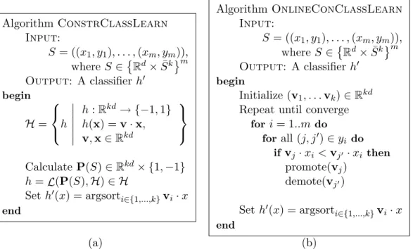
Ultraconservative algorithms for learning multi-class classifiers were introduced to provide a frame-work for developing and analyzing online algorithms for multi-class classification (Crammer and Singer, 2000a). Using an underlying representation of a single linear prototype per class, the classifier is (again) a winner-take-all function over the prototypes,h(x) = argmax_iwi·xi.

Ultraconservative algorithms are online, mistake driven algorithms. At each iteration, it per-forms weight vector updates,wi ←wi+τix, by discovering appropriateτi based only on the current

hypotheses and the new example. To be ultraconservative,τi6= 0 only when there was an “error”

with respect to classi. Specifically,τi <0 only if classiis in an error set,E={i6=y|wi·x≥wy·x}

when the correct label is y, and τy >0. A class in the error set would be predicted by the

winner-take-all label over the correct class. Therefore, individual updates will always move to correct that “error”. Of course, the challenge is to assign τ = (τ1, . . . , τk) collectively so that the resulting

algorithm will converge to a desirable solution. The choice of assignment produces different online algorithms.

Perhaps the simplest ultraconservative online algorithm is an extension of the perceptron algo-rithm, whereτi =−1/|E|for all classes i∈E,τy = 1, and τi = 0 otherwise. A second extension of

the perceptron is found when τi =−1 only when i= argmaxi6=ywi,τy = 1, andτi = 0 otherwise.

Additional choices depend not only on the error set, but on the values of the weights.

A further extension of this idea, the Margin Infused Relaxation Algorithm (MIRA) is presented in (Crammer and Singer, 2000a). Motivated by maximum-margin principles that lead to the discovery of a minimum-norm weight vector (satisfying large margin criteria), at each iteration, MIRA chooses how much to augment each class weight vector in such a way to minimize the norm of the resulting weight vectors. MIRA, in addition to being an ultraconservative online algorithm, converges at a rate inversely proportional to the optimal margin and an aggressiveness parameter of the algorithm.

(31)

2.4

Support Vector Machine

In its basic form, the support vector machine (SVM) finds the unique linear separation of two point sets such that the distance (margin) of the closest example to the decision boundary is maximized. This maximum-margin principle was introduced in the binary setting (Vapnik, 1995; Cortes and Vapnik, 1995) and recently extended to the multi-class setting (Weston and Watkins, 1999; Crammer and Singer, 2001a). For this brief introduction, we neglect the use of a threshold used for the classifiers but note that it is straightforward to add thresholds in all of the following cases.

2.4.1 Binary SVM

In the binary setting, given examples S = ((x1, y1), . . . ,(xm, ym)), where each (xi, yi) ∈ Rd×

{−1,1}, The SVM for finds the vectorw∈Rd for a linear decision function

h(x) = sign(w·x),

represented by wto maximize the minimum margin on the data set. Specifically,

w∗= argmax w∈Rd min (x,y)∈Sρ(w,x, y) = argmax_w_∈_Rd min (x,y)∈Sy w ||w||2 ·x

where the distance between each example and the decision boundary is represented by themargin, ρ(w,x, y) =y

w

||w||2 ·x

. The vector w∗ achieving maximum margin separation is written as an optimization problem,

maximizewˆ,ρ ρ

subject to: yi( ˆw·xi)> ρ ∀i

||wˆ||2 _{= 1} _,

(2.6)

where the goal is to find the maximum distanceρ. Although the above optimization problem has non-linear constraints, the solution can be found via an alternate quadratic optimization problem with linear constraints by dividing both sides of both constraints byρ, and rewritingw= wˆ_ρ. Then, ρ can be eliminated from the objective and the constraints and the optimization problem becomes

(32)

minimizew 1₂||w||2

subject to: yi(w·xi)≥1 ∀i

(2.7)

These two optimization problems are known as the the primal problems. However, due to the potentially large number of (general) linear constraints (derived from the examples), it is often more efficient to solve thedual problem. The dual is derived by writing out the Lagrangian (see (Boyd and Vandenberghe, 2003) for an introduction to convex optimization and the Lagrangian dual formulation), L(w, α) = 1 2||w|| 2₋ m X i=1 αi(yi(w·xi)−1) (2.8)

It is easy to see that if αi ≥ 0 for all i, then at the point, w∗, where the primal achieves

minimum value,L(w∗, α)≤ 1₂||w∗||2_{. Thus}_g₍_α_{) = min}

wL(w, α)≤L(w∗, α)≤ 1₂||w∗||2 is a lower bound to the optimal. The Lagrangian method prescribes to maximizeg(α) to obtain the optimal value. Furthermore, the maximum value maxαg(α) = 1₂||w∗||2, is optimal because the

Karush-Kuhn-Tucker (KKT) conditions specify that if a saddle point (i.e. maxαminwL(w, α) exists, then thewat that point is optimal.

For the maximum margin case, g(α) = minwL(w, α) is easy to compute by setting the deriva-tives of L(w, α) with respect tow to zero,

∂L(w, α) ∂wk =wk− m X i=1 αiyixik = 0.

As a result,wis written as a summation over the input examples,

w=

m

X

i=1

αiyixi

Finally, after plugging winto the Lagrangian, the dual objective function becomes

g(α) = min w L(w, α) = minw 1 2||w|| 2₋ m X i=1 αiyiw·xi+ m X i=1 αi = 1 2 m X i=1 αiyixi ! ·   m X j=1 αjyjxj  − m X i=1 αiyi   m X j=1 αjyjxj  ·xi+ m X i=1 αi =−1 2 m X i=1 m X j=1 αiαjyiyj(xi·xj) + m X i=1 αi (2.9)

(33)

Finally, the dual form of the SVM optimization problem can be formulated with a quadratic objective and linear constraints.

maximizeα −1₂Pmi=1

Pm

j=1αiαjyiyj(xi·xj) +Pmi=1αi

subject to: αi ≥0 1≤i≤m

(2.10)

There are many extensions to the basic SVM classifier and optimization-based learning algo-rithm presented here. It is straightforward to consider hypotheses of the form h(x) = w·x+b, with a threshold b ∈ _R, by using one additional constraint, Pm

i=1αiyi = 0. It is also relatively

straightforward (in the binary case) to extend the algorithm to deal with a limited amount of noisy data, by adding soft constraints to the optimization problem. Specifically, by allowing a certain weight of the data to realize negative margin, the optimization function can be rewritten as,

minimizew 1₂||w||2+CPn_i ξi

subject to: yi(w·xi)≥1−ξi ∀i

ξi≥0 ∀i,

(2.11)

whereC penalizes the weight that the soft solution can relax the pure constraints. As before, this can be written and solved in the dual.

Finally, the power of the SVM classifier comes not only from the large margin principle, but also from the ability to implicitly represent complex functions using kernels. There are many texts on this subject (Vapnik, 1995; Cortes and Vapnik, 1995; Herbrich, 2001; Scholkopf and Smola, 2001). Throughout this thesis, we omit details of using Kernel functions with the learning algorithms introduced and focus on the linear setting. However, we will mention their applicability when needed.

2.4.2 Multi-class SVM

Recent work has produced the multi-class SVM (Bredensteiner and Bennett, 1999; Weston and Watkins, 1999) by directly representing the multi-class problem in the primal constraints. To learn a multi-class classifier, h(x) =argmaxj∈{1,...,k} ∈ wj ·x, it suffices to find a set of weight vectors

w= (w1, . . . ,wk), wherewj ∈Rdsuch thatwy·x≥wj·xfor allj 6=y. From this intuition, we wish

(34)

This can be accomplished by maintaining the appropriate constraints in the primal minimizew 1₂||w||2

subject to: wyi·x−wj·x≥1 ∀i∈ {1, . . . , m} ∀j ∈ {1, . . . , k} \yi

(2.12)

Just as in the binary case, one can add slack variables to the optimization to deal with noisy data. The following approach adds a single slack variable per constraint, and is motivated by considering minimizing a (regularized) hinge loss (see (Weston and Watkins, 1999; Weston, 1999) for details), minimizew 1₂||w||2+CPmi=1 P j6=yiξ j i subject to: wyi·x−wj·x≥1−ξ j i ∀i∈ {1, . . . , m}, ∀j∈ {1, . . . , k} \yi ξ_ij ≥0 ∀i∈ {1, . . . , m}, ∀j∈ {1, . . . , k} \yi (2.13)

2.5

Multi-Prototype Support Vector Machine

The multi-prototype SVM is a multi-class classifier introduced in (Aiolli and Sperduti, 2005b). In training, we are given a labeled training set S = {(x1, y1), . . . ,(xn, yn)}, where xi ∈ X and

yi ∈ Y ={1, . . . , k}the corresponding class or label. In the multi-prototype setting, the underlying

scoring function of the linear multi-class setting is generalized to a set of linear scoring functions. As a result, it is able to represent more complex functions.

A multi-prototype classifier is a function h:Rd→ Y defined by over a set of scoring functions

parameterized by prototypes, w = (w1, . . . ,wR) ∈ Rd×R. Each prototype represents a scoring

function wr·x indicating the similarity between x and prototype r. In addition, we introduce a

many to one mapping C : {1, . . . R} → Y, from prototypes to classes, where C(r) represents the class associated to prototyper. This mapping associates each prototype to its output class. Then the decision rule (a.k.a. winner-take-all rule)

h(x) =C( argmax

r∈{1,...R}

w· · ·x), (2.14)

(35)

also be considered a sub-case of the same family of classifiers with a scoring function based on the distance between the example and the prototype.

Next, we define the set of positive prototypes for a class y as the set of prototypes P_y = {u| C(u) =y} and the set ofnegative prototypes as Ny ={v| C(v)6=y}. Following this, a natural

definition for the margin in the multi-prototype is ρ(x, y|w) = max u∈Py wu·x−max v∈Ny wv·x (2.15) = max u∈Py min v∈Ny ρuv(x|w). (2.16)

whereρuv(x|w) =wu·x−wv·xforu∈ Py andv∈ Ny. Notice thatρ(x, y|w) is greater than zero

if and only if the examplexis correctly classified. This definition reduces to the multi-class margin defined for the SVM case (Crammer and Singer, 2000a) when there is only a single prototype per class.

Now, let l : R → R+ a decreasing and non-negative loss function. The loss for the example

(x, y) is defined as L(x, y|w) =l(ρ(x, y|w)) = min u∈Py max v∈Ny l(ρuv(x|w)) (2.17)

To measure the actual error, one can set the loss to be the indicator function l(ρ) = I(ρ), where I(ρ) = 1 whenρ≤0 and 0 otherwise. ThenL(x, y|w) = 1 and there is an error if and only if there is no positive prototype ˆu∈ P_y of the correct classy that has higher score than all the prototypes inNy. Other losses can be used here as well.

According to the structural risk minimization principle used for SVM (Vapnik, 1998), we wish to find the optimal solution that is both reasonably ’simple’ and minimizes the empirical risk, i.e. we are searching for a hypothesis

w∗ = argmin w∈Rd×R X (x,y)∈S L(x, y|w) +µR(w) = argmin w∈_Rd×R X (x,y)∈S min u∈Py max v∈Ny l(ρuv(x|w)) +µR(w) (2.18)

where R(w) is a regularization term weighted by µ, the trade-off parameter. This optimization problem is non-convex when more than one prototype per class is used, and therefore may have many local minima.

(36)

2.5.1 The Multi-Prototype SVM Solution

The multi-prototype SVM (MProtSVM), proposed in (Aiolli and Sperduti, 2005b) uses the hinge loss and a quadratic regularization term. Basically, they pose the problem in Equation 2.18 is posed as a (non-convex) constrained optimization problem

minimize_w_,_ξ 1₂||w||2₊_CPn

i ξi

subject to: maxu∈P_yiwu·xi−maxv∈N_yiwv·xi ≥1−ξi ∀i

ξi ≥0 ∀i

(2.19)

where the constraints dictate that for each example (xi, yi), there exists a positive prototype,

u ∈ P_y, that achieves higher score than all negative prototypes, v ∈ N_y. Otherwise a loss ξi

corresponding to the hinge loss is suffered.

Furthermore, the MProtSVM reduces this problem to a sequence of convex problems by intro-ducing additional variables, ξ_i = {ξ_i1, . . . , ξ|Pi|

i }, πi = {π1i, , . . . , π

|Pi|

i }, and θi, i ∈ {1, . . . , n}, to

break up the constraint in Equation 2.7 in the following way: minimize_w_,_ξ_,_π_,_θ ₂1||w||2₊_CPn i πi·ξi subject to: wv·xi≤θi ∀i, v∈ Nyi wu·xi ≥θi+ 1−ξiu ∀i, u∈ Pyi ξ_iu ≥0 ∀i, u∈ P_y_i πi∈[0,1]|Pi|, ||πi||1= 1 ∀i, (2.20)

where the vectors,πi, are assignment vectors to choose which slack variables (ξiu = [1−ρuv˜(xi|w)]+

at the optimum) to include in the objective. Intuitively, this corresponds to selecting which pro-totypes will incur loss. For any fixed, π, the above optimization is convex. Notice that if πi is

appropriately chosen (i.e. π_iu= 0 unless u= ˜u= argmax_u∈Pyw

∗

u·x), then the optimization

prob-lem reduces to the one in Equation 2.7, as ξ_iu, u6= ˜u does not affect the objective. Alternatively, if πi is the uniform distribution (πui = |P1_yi|), then the problem reduces to a single prototype per

class setting since the problem is symmetric and all the prototypes for each class collapse into one. The MProtSVM exploits this intuition and performs a stochastic search for the optimal as-signment. This requires the algorithm to (partially) solve a number of convex problems where the assignment is fixed. Although heuristic strategies are proposed to avoid the full computation of

(37)

these dual problems, it can be onerous, or even impossible, to find a solution when the number of examples is large. Moreover, since the reduced problems are indirectly solved via the dual repre-sentation, it is possible that the algorithm will spend most of the time on solutions unrelated to the true optimal in the primal. In Chapter 4, we present an alternate solution to this problem.

2.6

Structured Output Classification

In many prediction tasks, the output is composed of multiple dependent variables. It is often the case that dependencies can be modeled using a structgured representation, such as a sequence, tree, or graph. Indeed, the structure in the output can strictly adhere to a known form, or can be implicitly defined based on some background knowledge or even the data at hand. In some sense, the structured output problem is loosly defined, however two key aspects help to define the problem — it involves tasks that clssify a collection of variables, and the structure biases and constrains the output variables. In this section, we review work related to Chapters 5 and 6.

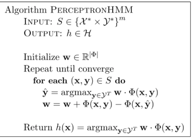
2.6.1 Perceptron Hidden Markov Models (and CRFs)

Recently, the perceptron algorithm was extended to the structured output domain, where the strcutre was represneted by a Condition Random Field (CRF). Here, for clarity, we follow (Collins, 2002) and describe its application using Hidden Markov Models (HMMs).

The Perceptron HMM is a discriminnant learning aprpoach for learning the parameters of a HMM. More precicly, the representation of the HMM-like classifier is identical to the representation of a HMM with the exeption that the parameters are no longer restricted to be probabillities. Instead, the parameters are viewed as a feature set and probability estimateion is replaced with a (linear) similarity score. This method uses the general discriminant model for learning from Section 2.2.

A HMM represents a probability distribution of a sequental output y∈(y1, . . . , yT)∈Y˜T =Y

given inputx= (x1, . . . , xT) sin ˜XT =X as

P(x,y) =

T

Y

t=0

P(yt|xt)P(yt|yt−1)

(38)

function, h(x) = argmax y∈Y˜T logP(y|x) = argmax y∈Y˜T w·Φ(x,y), where examplex is lengthT.

In practice, the higest scoring output is efficently infered by thte Viterbi algorithm. Fotunately, the viterbi algorithm does not depend on the values of the numbers, only the relationships drawn from the HMM structuree. As a result, the viterbi algorithm can find thehighest scoring assignemt even when the numbers are not probabilies. In (Collins, 2002), this observation made it possible to include inference in an online procecdure.

The Perceptron HMM is an online, mistake-driven algorithm where, at each iteration, the highest scoring output ˆy= argmax_yΦ(x,y) is compared witht the correct outputy. A perceptron-like update rule is performed only ify6= ˆyand a mustake was made. See Algorithm 2.1 for details. As a result, a pricipled way to learn parameters of a model derived from a probabilistc framewrok was found. Furthermore, notice that it is possible to view this algorithm as an instance of using the perceptron in the general discriminant framework in Section 2.2. Specifically, with Φ(x,y,yˆ) = Φ(x,y)−Φ(x,yˆ), the update above is simply

w=w+ Φ(x,y,yˆ),

exactly the perceptron update in the transformed “pseudo” example space. AlgorithmPerceptronHMM

Input: S∈ {X∗× Y∗}m Output: h∈ H

Initializew∈_R|Φ|

Repeat until converge

for each(x,y)∈S do

ˆ

y= argmax_y_∈YT w·Φ(x,y)

w=w+ Φ(x,y)−Φ(x,yˆ)

Returnh(x) = argmax_y∈YTw·Φ(x,y)

(39)

2.6.2 Maximum-margin Markov Networks

Maximum-margin Markov Networks (M3), introduced in (Taskar, Guestrin, and Koller, 2004), learn the parametes of a markov network in such a way to maximize the margin of the final classifer. Similarly to learning the parameters of a HMM using perceptron, this method eliminates the necessity of a probabliistic interpertation of the final classifer. The M3 extends learning HMMs with perceptron to the more expressive markov framework and learns in a way to maximize the margin of the resultant classifer.

A Markov network (also known as a Markov random field) representes a general probablistic framwork. It is defined as a graph G = (V,E) composed of a set of random variables, V = (v1, . . . , vT) ∈ VT and a set of pairwise dependecies between variables, E, and a parameter set.

In the current context, we describe the parameter set as a set of weights and potential functions. Specifically, we define a set of feature (or potential) functions as Φ = (φc|c is a clique inG) and a

weight setw= (wc|cis a clique inG). Hereφc :VT → {0,1}represent induvidual features such as

“v1 = 1 andv2 = 0” andwc∈Rare respecitve weights. The feature vector, Φ :VT → {0,1}|Φ|, and

weight vector, w, are the concatentation of the φc andwc, respectively. For a detailed description

of Markov random fields, see (Smyth, 1997). The probability defined for an assignment, v of all random variables V is written as

P(v) = 1 Z

Y

c

2wcφc(v)_, whereZ is a normalizzing constantZ =P

v Q

c2wcφc(v). Clearly, I have written these terms in the

exponentail to higlight that it is a log-linear model, and thus logP(v) =w·Φ(v).

In (Taskar, Guestrin, and Koller, 2004), as well as here, we assume that V = ˜X∗_×_Y_˜∗ ₌_{X × Y,}

and v= (x,y) and classify accorkding to the maximum liklihood estimate h(x) = argmax y P(y|x) = argmax y P(y,x) = argmax y logP(y,x) = argmax y w·Φ(x,y), by assuming a uniform priorP(y) =P(y0) for all y,y0 ∈ Y.

As in (Collins, 2002), by elimiinianting the requirement that the parameters of this model conform to a probability distribution, one can approach learning markov networks as a

(40)

gen-eral classification problem. In (Taskar, Guestrin, and Koller, 2004), the margin is defined as the difference in the correct output score and the highest scoring (incorrect) label, (ρ(x,y,w) =

wΦ(x,y)−maxy0₆₌_yΦ(x,y0))/||w||2. Then, the maximum margin solution is written as an

otimi-aztion problem, minimize_w_,_ξ 1₂||w||2₊_CPn i ξi subject to: w·Φ(xi,yi)−w·Φ(xi,y0)≥∆(yi,y0)−ξi ∀i, ∀y0 6=yi ξi ≥0 ∀i (2.21)

where ξi are defined per example. It is important to note that there is a single slack variable per

exampl. This choice is crutial, and is derived from a special loss..

The number of constraints in the above optimization problem grows exponentially with the number of variables. As a result, standard optimization techniques do not scale to even relatively small output problems. In (Taskar, Guestrin, and Koller, 2004), they present a solution by re-writing the dual optimization function and decopoliing the problem. Specifically, the dual is written by writing out the Lagrangian functional for the above problem, as

maximizeα Pn_i₌₁P_yαi,y∆(yi,y) − 1₂ Pn i=1 P yαi,y(w·Φ(xi,yi)−w·Φ(xi,y)) 2 subject to: P yαi,y= 1 ∀ i= 1, . . . , n αi,y≥0 ∀ i= 1, . . . , n, ∀y, (2.22)

where we sum over all possibley assignments given the structure.

Both the size of the optimization function, and the number of constraints depend on the size of the output. In fact, an output of sizeL produces kL outputs when each of the variables can take one ofk values. This produces an unsolvable optimzation solution. To solve this problem, a very clever observation was made — that the, α, assignments are a probability distribution since they sum to a constant,C, and they are all non-negative. Under this view, the objective function is the sum of expectations of ∆(yi,y) andρ(x,yi,y), and because it is derived from a CRF model, it can

be factored based on the cliques. If the cliqe size is small, then the optimization problem can be factored into small sized components and solved efficiently.

(41)

2.7

Generalization Bounds

Learning theory deals with complexity measures associated with the learning problem such as the computation complexity and thesample complexity. Computation complexity bounds the running time for an algorithm to halt, while the sample complexity bounds the number of examples (sam-ple size) required for an algoirthm to perform to a specified performance in the future. Sam(sam-ple compleixty bounds are typically used to measure the expected future performnace by bounding the expected generalization error. In this section we review some generalization bounds that are used througout this disseration.

2.7.1 PAC bounds

In the probably approximatley correct (PAC) framework, the learner attempts to learn an -accurate hypothesis with confidence 1−δin polynomial time (Valiant, 1984; Blumer et al., 1989). A learning algorithm,Lis a PAC learning algorithm if, in polynomial time,poly(m,1,1_δ), it discovers a hypothesis h=L(S,H) using at most m =poly 1,1_δ

examples, such that the probability that h has large error,

P(E(h)≤)>1−δ.

A general approach to derive generalization bounds is to measure the difference between ob-served (emperical) error and the true error of any given hypothesis. Specifically, given a set of m examples,S, drawn i.i.d. fromDX ×Y, the differece,|E(S, h)−ED(h)|is small, with high probability.

It is easy to bound this quantity if h is fixed andS are randomly drawn using classical statistical techniques such as the Chernoff bound. Whenhcomes from a larger hypotehsis class and is chosen more carefully, one can use the complexity of the hypothes