Hedging Credit Risk Using Equity
Derivatives
Paul Teixeira
School of Computational and Applied Mathematics
University of the Witwatersrand
A dissertation submitted for the degree of
Master of Science in
Advanced Mathematics of Finance
Declaration
I declare that this is my own, unaided work. It is being submitted for the Degree of Master of Science to the University of the Witwatersrand, Johannesburg. It has not been submitted before for any degree or examination to any other University.
(Signature)
Abstract
Equity and credit markets are often treated as independent markets. In this dissertation our objec-tive is to hedge a position in a credit default swap with either shares or share options. Structural models enable us to link credit risk to equity risk via the firm’s asset value. With an extended version of the seminal Merton (1974) structural model, we value credit default swaps, shares and share options using arbitrage pricing theory. Since we are interested in hedging the change in value of a credit default swap dynamically, we use a jump-diffusion model for the firm’s asset value in order to model the short term credit risk dynamics more accurately. Our mathematical model does not admit an explicit solutions for credit default swaps, shares and share options, thus we use a Brownian Bridge Monte Carlo procedure to value these financial products and to compute the delta hedge ratios. These delta hedge ratios measure the sensitivity of the value of a credit default swap with respect to either share or European share option prices. We apply these delta hedge ratios to simulated and market data, to test our hedging objective. The hedge performs well for the simulated data for both cases where the hedging instrument is either shares or share options. The hedging results with market data suggests that we are able to hedge the value of a credit default swap with shares, however it is more difficult with share options.
Acknowledgements
I would like to express my sincere appreciation to my supervisors, David Taylor and Lawrence Madzwara, for providing me the opportunity to do this research and for their helpful insights into aspects of the dissertation. I gratefully appreciate Dr. Jordens for editing my dissertation. I would also like to thank my parents, family and fellow students for their support and encouragement.
Contents
1 Introduction 1
1.1 Background to the Credit Derivatives Market . . . 1
1.2 Credit Risk and Equity . . . 2
1.3 Credit Risk Models . . . 3
1.4 Research Objectives . . . 4
1.5 Structure of the Dissertation . . . 5
2 Mathematical Framework 6 2.1 Introduction . . . 6
2.2 Arbitrage Pricing Theory . . . 6
2.2.1 Financial Market Model . . . 6
2.2.2 Equivalent Martingale Measure . . . 8
2.2.3 Arbitrage-Free Pricing of Contingent Claims . . . 11
2.3 Financial Securities Dependent on the Default Event . . . 12
2.3.1 General Credit Risk Model . . . 12
2.3.2 Arbitrage-Free Valuation Formula . . . 13
2.3.3 Reduced-Form Model . . . 13
2.3.4 Structural Model . . . 14
2.4 Discussion . . . 14
3 Credit Default Swaps 15 3.1 Introduction . . . 15
3.2 Credit Risk . . . 15
3.3 Credit Ratings . . . 16
3.4 Credit Derivatives . . . 16
3.5 Credit Default Swap . . . 16
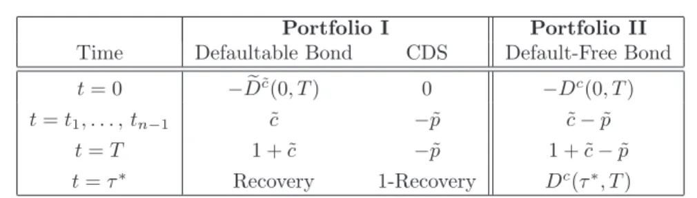
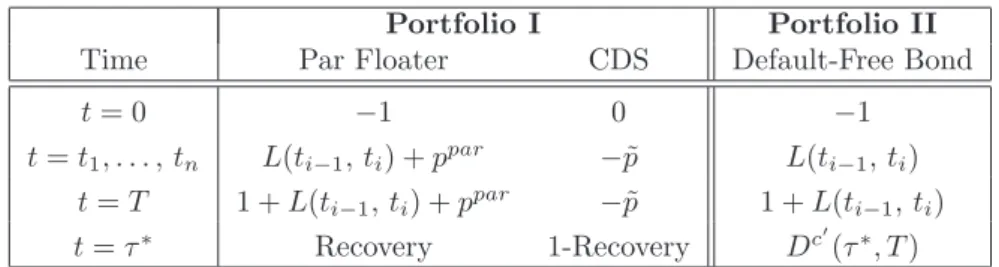
3.6 Replication-Based CDS Pricing . . . 18
3.6.1 Replication Instruments . . . 18
3.6.2 Short Positions in Bonds . . . 19
3.6.3 CDS Replicating Strategies . . . 20
3.7 Bond Price-Based CDS Pricing . . . 22
3.7.1 Bond Price-Based Framework . . . 23
3.7.2 Extensions to Situation where Defaults can happen at any Time . . . 24
3.7.3 CDS Pricing . . . 25
3.8 Generic CDS Pricing Model . . . 26
3.9 Discussion . . . 27
4 Structural Models 28 4.1 Introduction . . . 28
4.2 The Merton Model . . . 28
4.3 Extensions to the Merton Model . . . 33
4.3.1 Capital Structure . . . 33
4.3.2 Default Barrier . . . 34
4.3.3 Stochastic Interest Rates . . . 36
4.3.4 Unpredictable Default Time . . . 37
4.3.5 Discontinuous Firm’s Asset Value Process . . . 37
4.4 Parameter estimation . . . 38
4.5 Our Model . . . 42 ii
CONTENTS iii
4.6 Discussion . . . 45
5 Pricing and Estimation 46 5.1 Introduction . . . 46
5.2 Principles of Monte Carlo Methods . . . 46
5.3 Brownian Bridge . . . 49
5.4 A Brownian Bridge Simulation Procedure for Pricing CDS Premiums . . . 50
5.4.1 Model Description and the CDS Pricing Formula . . . 51
5.4.2 Outline of the Monte Carlo Brownian Bridge Method to Price CDS premiums 52 5.4.3 Conditional First Passage Time Distribution . . . 53
5.4.4 Decomposition of the CDS Pricing Formula . . . 54
5.4.5 Sampling a First Hitting Time in an Inter-Jump Interval . . . 57
5.4.6 The Simulation Algorithm to Price the Premium of a CDS . . . 58
5.4.7 The Brownian Bridge Simulation Algorithm to Value a CDS . . . 59
5.4.8 The Brownian Bridge Simulation Algorithm to Price Equity . . . 60
5.4.9 Numerical Results of the Brownian Bridge Simulation Algorithm . . . 61
5.5 Valuing Equity Options by a Monte Carlo Linear Regression Approach . . . 63
5.5.1 The LSM Algorithm . . . 64
5.5.2 Numerical Comparison of Basis Functions . . . 65
5.6 Estimation of parameters . . . 66
5.6.1 The Nelder-Mead Simplex Method . . . 67
5.6.2 The Nelder-Mead Algorithm . . . 67
5.7 Discussion . . . 69
6 Numerical Analysis 70 6.1 Introduction . . . 70
6.2 Effects of Credit Risk on CDS, Equity and Equity Derivatives . . . 70
6.3 Hedging . . . 71
6.4 Delta Hedging . . . 74
6.4.1 A Measure for the Efficiency of a Delta Hedge . . . 76
6.4.2 Gamma Hedge . . . 77
6.5 Empirical Tests . . . 78
6.5.1 Method . . . 79
6.5.2 Testing the Delta Hedging Strategy with Simulated Data . . . 81
6.5.3 Data . . . 82
6.5.4 Results . . . 83
6.6 Conclusion . . . 92
6.7 Further Research Directions . . . 93
A Jump Processes: Miscellaneous Results 94 A.1 Itˆo’s Formula for Diffusions with Jumps . . . 94
A.2 Girsanov Theorem for Jump-Diffusion Processes . . . 95
A.3 The Firm’s Value Process under the Risk-Neutral Measure . . . 96
B First Passage Time 98 B.1 The Hitting Time of a Standard Brownian Motion Process . . . 98
B.1.1 Distribution of the Pair (Wt, Mt) . . . 98
B.1.2 Distribution of Mt andτM, b∗ . . . 100
B.1.3 The Distribution of the pair (Wt, mt) . . . 100
B.1.4 Distribution of mtandτm, b∗ . . . 101
B.2 The First-Hitting Time for a Brownian Motion with Drift . . . 101
B.3 The First-Hitting Time of a Geometric Brownian Motion Process V to a Lower Barrier b . . . 102
C Miscellaneous 104 D Hedging Results 105 D.1 Simulated Delta Hedge Results . . . 105
D.2 Empirical Delta Hedge Results . . . 108
Chapter 1
Introduction
1.1
Background to the Credit Derivatives Market
The rise in credit related events (i.e. bankruptcy of firms, default and deterioration of the credit quality of corporate and government bonds) throughout the financial world over the past decade has been met with a commensurate increase in interest in derivatives which depend in value solely on credit risk1. Until recently there did not exist risk management products for credit risk. The market for credit derivatives2 began slowly in the early 1990’s, sparked by the need to keep pace with the increasing demand for other over-the-counter derivative products. The sheer volume of business swamping the market meant that financial institutions could no longer rely on taking collateral or making loss provisions to manage their credit risk. They strived for a way to lay off illiquid credit exposures and to protect themselves against defaulting clients.
Traditionally, credit was sourced in the new issue market and placed with the end investors, where it remained irrevocably linked to the asset with which it was originally associated. With the innovation of credit derivatives it is now possible to separate credit risk from any financial obligation (i.e. loans, bonds, swaps) and manage it just like any other asset. The credit derivative tool kit has revolutionized credit risk management and fundamentally modernised the credit market. Before the advent of credit derivatives, credit risk management meant a strategy of portfolio diversification backed by credit line limits, with occasional sale of positions in the secondary market. These strategies are inefficient, largely because they do not separate the management of risk from the asset with which the credit risk is associated. Credit derivatives are significant as they allow the risk manager to isolate credit risk and manage it discreetly without interfering with customer relationships. They also form the first mechanism via which short sales of credit instruments can be performed with reasonable liquidity. For example, it is impossible to short-sell a bank loan, however this can be achieved synthetically by buying a credit derivative offering credit protection. Credit derivatives allow investors to be synthetically exposed to credit assets that were unavailable before, either because of regulations or because these assets were publicly restricted (e.g. bank loan).
The credit derivative market has experienced an exponential growth since its inception in the early 1990’s. The total market notional for 2006 is estimated at $20,207 billion (US dollars) and is predicted to increase to $33,210 billion by 2008, according to surveys by the British Banker’s Association (BBA) (see Barret & Ewan (2006)). Figure 1.1 shows estimates, from Barret & Ewan (2006), of the growth of the credit derivative market. It is not just the size of the market that has continued to grow, but also the diversity of credit derivative instruments. To highlight, a few recent products are: index trades, tranched index trades and equity-linked products. Single name credit default swaps (CDS) represent a substantial section of the market, according to the BBA 2006 survey, single name CDS represents 32.9% of the credit derivative market. The single name CDS is considered to be the fundamental instrument in the credit derivatives market, and is the focus of this dissertation. Since 1992, the International Swaps and Derivatives Association (ISDA) has standardised CDS contracts and other credit derivatives, allowing the involved parties to specify the terms of the transaction from a number of defined alternatives. Recently the ISDA has
1Credit risk is the risk of default on an obligatory payment. We give a thorough description of credit risk in
Chapter 3.
2We give a detailed definition of credit derivatives in Chapter 3, for now it can be thought of as a financial
instrument whose value depends on credit risk.
1.2. Credit Risk and Equity 2
published the 2003ISDA Credit Derivatives Definitions, which updates the 1999 version, and offers the basic framework for the documentation of privately negotiated credit derivative transactions. This standardisation has been a major development in the credit derivative market, since it has reduced legal ambiguities that hampered the market’s growth in its early stages. Growth in this market has also been spurred by banks’ recent endeavours to develop internal credit risk models to quantify regulatory capital requirements, which has been encouraged by the 1997 revised Basel Capital Accord and the new 2004 Basel II Capital Accord3. Banks have dominated the market as the biggest traders of credit derivatives. Other major market participants are securities firms, insurance companies and hedge funds.
1996 1998 1999 2000 2001 2002 2003 2004 2006 2008 (est.) 0 5,000 10,000 15,000 20,000 25,000 30,000 35,000 Year
Market Notional (USD billion)
Figure 1.1: Growth of the credit derivative market according to the British Banker’s Association 2006 survey.
1.2
Credit Risk and Equity
There have been several studies on the relationship between credit risk and equity, and it is widely agreed that there is a negative relationship between them. Vassalou & Xing (2004) and Charitou et al. (2004) concluded that there exists a statistically significant negative relationship between credit risk (as measured by the risk-neutral probability of default4derived from the Merton (1974) model) and stock returns, and this relationship is more significant for firms with a high default probability. Elizalde (2005) assumed aglobal market credit risk factor inherent in all bond prices. Using linear regression, he found that this global market credit risk is negatively correlated with equity indices (S&P 500 and Dow Jones). This negative relationship between credit risk and equity prices is intuitive. As a firm’s credit risk increases, the firms financial health decreases (its propensity to default increases) and equity investors will become sceptical of realising a return on their investment, resulting in share prices decreasing. By construction, credit default swaps are the financial instruments with the most accurate reflection of a firm’s credit risk5. By regressing CDS premiums on several equity factors, Zhang et al. (2005) found that equity returns are statistically significant in explaining the change in CDS premiums. By calculating the daily lead-lag cross-correlation coefficients, Acharya & Johnson (2005) and Bystr¨om (2005) found that share price changes lead CDS premium changes, that there is an inverse relationship between the two, and that this inverse relationship is strongest when the lag is zero.
The main objective of this dissertation is to quantify this relationship between CDS premium changes and stock returns in order to hedge6a position in a CDS with an equity position. To my knowledge the closest related studies to this objective are by Yu (2005) and Schefer & Strebulaev
3The set of regulatory banking capital adequacy requirements, compiled by the Bank for International Settlements
(BIS) Basel Committee on Banking Supervision.
4This measure of credit risk will be discussed in detail in Chapter 4.
5In Chapter 4 we discuss credit default swaps in detail. There it is shown why it is value is considered to be the
most accurate reflection of credit risk.
6A hedge is a trading strategy designed to reduce risk, the variability of the value of the position being hedged.
1.3. Credit Risk Models 3 03/01/2003 03/01/2005 03/01/2007 2.5 3 3.5 4 4.5 5 5.5 Date Plot (a) 03/01/2003 03/01/2005 03/01/2007 3.4 3.8 4.2 4.6 5 5.4 Date Plot (b) 03/01/2003 03/01/2005 03/01/2007 2 3 4 5 6 7 Date Plot (c) 03/01/2003 03/01/2005 03/01/2007 3 4 5 6 7 8 Date Plot (d)
Figure 1.2: Times series plots of daily 5 years CDS premiums and daily share prices (the natural logarithm is taken of both time series for visual comparison) for 4 different NYSE listed companies: Boeing (Plot (a)), Daimler Chrysler (Plot(b)), Ford (Plot(c)) and General Motors (Plot (d)). The red line represents 5-yr CDS premiums and the blue line represents share prices.
(2004). Yu (2005) investigates how profitable their capital structure arbitrage trading strategy is. Capital structure arbitrage attempts to profit from temporary relative mispricings between market CDS spreads and theoretically implied equity CDS spreads. In this strategy they hedge their trading strategy with an equity position. However, the focus of this paper is the realised trading profit and not on the ability of their model to hedge their CDS position. Schefer & Strebulaev (2004) calculated hedge ratios, that measured the sensitivity of bond prices with equity, from the Merton model, and found that they successfully predict market sensitivities. To further illustrate the relationship between the CDS market and the equity market, four NYSE (New York Stock Exchange) listed companies’ daily share prices are plotted in figure 1.2, with their corresponding daily 5 year CDS premiums. From these plots it can be seen there is a definite negative relationship between the two. Each of the firm’s cross-correlation7(between the natural logarithm8of daily 5yr CDS premiums and the natural logarithm of daily share price) coefficientsρalso reveal a negative relationship: Boeingρ=−0.9662, Daimlerρ=−0.8582, Ford ρ=−0.9005 and General Motors ρ=−0.9392.
1.3
Credit Risk Models
There exists two classes of credit risk models: structural and reduced form. Structural models originated with Black & Scholes (1973), and Merton (1974), and reduced form models with Jarrow & Turnbull (1995). Structural models are built on the premise that there is a fundamental process
7Pearson’s product-moment cross-correlation with zero lag. This correlation coefficient ρ∈[−1,1], measures
the linear dependency between two random variables. The correlation coefficient is 1 in the case of an increasing linear relationship, -1 in the case of a decreasing linear relationship, and some value in between in all other cases, indicating the degree of linear dependence between the variables. The closer the correlation coefficient is to either -1 or 1, the stronger the correlation between the random variables.
8In general, when calculating the correlation between two financial assets, we look at the natural logarithm of
the assets’ price, because a common assumption is that financial asset prices follow a log-normal distribution. Thus the natural logarithm of financial asset prices follow a normal distribution, which is the natural distribution of the random variables when calculating the Pearson’s product-moment cross-correlation coefficient.
1.4. Research Objectives 4
Vt, interpreted as the total value of the assets of the firm at timet. The firm’s asset value Vt is
the driving force behind the dynamics of the prices of all the securities issued by the firm (equity and debt), and all claims on the firm’s value are modelled as derivative securities with the firm’s valueVtas the underlying. In the structural framework, default is triggered when the asset value
Vt is insufficient to pay back the outstanding debt. This is modelled as Vt crossing some default
threshold barrier bt. From the structural model one can model both credit risk and equity, the
fundamental link being the firms’ asset valueVt. This is the reason why we will focus on structural
models in this dissertation. In a reduced form framework, default is modeled by a default process. The default process is usually defined as an exogenous one-jump process which can jump from no-default to default. Reduced form models use market prices of the firms defaultable instruments (such as bonds or credit default swaps) to extract their default intensity (the jump intensity) which can be used to calculate default probabilities and prices of other defaultable instruments. The value of the firm’s assets and its capital structure are not modelled at all. They rely on the market as the only source of information regarding the firms credit structure (without considering any credit related information included in balance sheets or equity prices).
1.4
Research Objectives
There are three objectives that will be considered in this dissertation. Firstly, to establish a theoretical relationship between CDS values and equity prices, via the structural model framework and calculate the sensitivity of CDS values to equity prices (hedge ratios). The second objective will be to quantify these sensitivities with market data. The third objective will be to test whether these sensitivities can be used to hedge exposure to a CDS position, with an equity position, either using an equity option or the underlying equity.
Since we are using the structural model approach, the theoretical values of credit default swaps, φt, stocks,St, call stock options9, ϕt, and put stock options ,ϕt, will be dependent on the firm’s
asset value Vt. The sensitivity of credit default swap values, φt, to stock prices, St, call stock
option prices,ϕt, and put stock option prices,ϕt, will be evaluated by using the following partial
derivatives10: ∂φt ∂St = ∂φt ∂Vt ∂Vt ∂St , (1.1) ∂φt ∂ϕt = ∂φt ∂Vt ∂Vt ∂ϕt, (1.2) ∂φt ∂ϕt = ∂φt ∂Vt ∂Vt ∂ϕt . (1.3)
The above partial derivatives give the rate of change of CDS values with respect to stock, call stock option and put stock option prices, with all the other independent variables in the CDS pricing formula remaining fixed. These partial derivatives will determine the number of shares, and options on shares, that are needed to hedge the change in value of a CDS. We will name these partial derivativesdelta hedge ratios. We will apply a simple hedging strategy according to these delta hedge ratios to determine if it is possible to hedge exposure to a CDS position with an equity position.
Intuitively, a credit instrument (eg. a corporate bond) should be used to hedge a CDS11. A less obvious approach would be to use a position in equity, since credit and equity markets are often considered to be distinct. By means of a structural credit risk model we are able to theoretically link these two markets. In Chapter 3, we will see that hedging a CDS with a credit instrument can be problematic or even impossible as there may not be any publicly available credit instruments. We analyse a novel alternative approach to hedging credit default swaps, by taking a position in the equity market. From this study we are also able to infer theoretical prices for equity (shares and share options) and credit default swaps from the credit and equity market, respectively. From these theoretical prices, it is possible to identify relative mispricings between theoretical (which has
9In this dissertation we only work with European options.
10We show in Chapter 6 that there is one-to-one relationship between CDS values, stock prices, stock option prices
and the firm’s asset valueV, under our structural model framework. Since there is this one-to-one relationship, equations (1.1), (1.2) and (1.3) hold.
11This is intuitive, since a CDS can be seen as insurance policy on a credit instrument, thus a natural hedging
1.5. Structure of the Dissertation 5
been inferred by a different market) and market prices, which is required to perform the capital structure arbitrage trading strategy.
1.5
Structure of the Dissertation
The three specific aims of this study are: to construct a mathematical model that will enable us to relate the credit and equity market dynamically, to examine methods of pricing of equity and credit products under our mathematical model, and finally calculate the delta hedge ratios and implement them with market data to asses if it is possible to hedge the value of a credit default swap with stock or stock options.
In the following, we briefly go over the content of each chapter. Chapter 2 outlines the math-ematical underpinnings of credit risk models. This framework is based on the asset valuation framework developed by Harrison & Pliska (1981). It is extended to account for assets that have defaultable payments. Chapter 3 gives a brief overview of credit derivatives and a thorough descrip-tion of credit default swaps and its intricacies. An approximate hedge-based pricing (replicadescrip-tion) strategy (Sch¨onbucher (2003)) of credit default swaps will be illustrated. A bond based pricing method (Hull & White (2000)), a popular method to price CDS, will also be explained. A generic CDS pricing formula will be presented, that is applicable to all credit risk models. Chapter 4 examines structural models. We review the seminal structural model, the Merton (1974) model, and comment on its strengths and weaknesses. We research extensions to this model, and analyse the significance of the additional features. We present our model that will be used to price and calculate the delta hedge ratios. We present several techniques available to estimate the parameters of a structural model. Chapter 5 we give the valuation formulae for CDS, stock and European stock options. Since our mathematical model does not admit explicit solutions for theses valuation formulae, we present Monte Carlo methods to calculate the valuation formulae. We investigate their computational accuracy and efficiency. We outline the calibration method which we used to estimate our model’s parameters. In Chapter 6 we examine hedging under different market as-sumptions. We then present the method to calculate our delta hedge ratios and outline the method to implement them to hedge a position in a CDS with stock or stock options. We then test this hedging scheme with simulated and market data. We conclude with an examination of the results from these tests.
Chapter 2
Mathematical Framework
2.1
Introduction
The purpose of this chapter is to lay down the mathematical framework and describe the arbitrage-free pricing technique for defaultable securities. This is not a thorough description of arbitrage-free pricing theory. For a technical account the interest reader is referred to Protter (2005). The following section highlights some of the main ideas concerning the arbitrage-free pricing technique fornon-defaultablecontingent claims. We will extend this arbitrage-free pricing technique to price defaultable contingent claims. From the general arbitrage-free framework for defaultable claims, we will characterise two major credit risk models: the structural model and the reduced form model.
2.2
Arbitrage Pricing Theory
An arbitrage opportunity exists if it is possible to make a risk-free profit. The absence of arbitrage opportunities in the financial market model is the fundamental economic assumption for asset pricing. By assuming the financial market model is arbitrage-free, portfolios having identical cash flows must have the same price. By constructing an appropriate portfolio which yields a riskless return over an infinitesimally small period of time, Black & Scholes (1973) concluded that to avoid arbitrage opportunities the portfolio’s instantaneous return must equal the prevailing risk-free rate. This observation led to their celebrated partial differential equation which can be explicitly solved for European vanilla options. The first mathematically rigorous framework for arbitrage-free pricing was developed by Harrison & Kreps (1979) and Harrison & Pliska (1981). We now review the main results of Harrison and Pliska, in order to extend these tools to price defaultable securities. For now, we assume all securities are non-defaultable and later in the chapter we include defaultable securities into the mathematical framework. All of the following definitions, propositions and theorems are taken from ˇSeli´c (2006) and Brigo & Mercurio (2006).
2.2.1
Financial Market Model
Consider a financial market with a fixed trading horizon [0, T]. On this time interval the uncertainty of the financial market is modelled by a filtered probability space (Ω,FT,F,P), P ∈P, where
Ω is the sample space set containing all possible outcomes, F is right continuous filtration, F =
{Ft: 0≤t≤T}(a dynamically evolving information structure),Pis the real world (or statistical)
probability measure assigned to event setsA∈FandPis a class of equivalent probability measures on (Ω,FT). The financial interpretation of modelling the uncertainty in a financial market with
aclass of equivalent probability measures, is that investors agree on which outcomes are possible, but their assignment of probability to these outcomes differ (see Musiela & Rutkowski (1997) for more details).
In the financial market there areK+ 1 primary traded securities. These primary securities do not pay dividends. The price processes of these securities are denoted1 byV ={V
t, 0≤t≤T}, whereVt= ¡ V0 t, Vt1, . . . , VtK ¢0
. We model these processes with strictly positive semimartingales
1In the usual Harrison & Pliska (1981) framework, the primary securities are stock, however under the structural
model the primary securities are the firm’s total assets.
2.2. Arbitrage Pricing Theory 7
(see Protter (2005) for the mathematical definition of a semimartingale stochastic process). Semi-martingales are conventionally used to model price processes as they are the most general stochastic process for which a stochastic integral can be reasonably defined. It can be shown (see Delbaen & Schachermayer (1998), Theorem 7.2) if the price processes are modelled by semimartingales and the model admits equivalent martingale measures, then our model is arbitrage-free2. The security indexed by 0 is the bank account process, and its price process evolves according to
dVt0=rtVt0dt, (2.1)
whereV0
0 = 1 andrtis the instantaneous risk-free short rate at timet. The solution of (2.1) is
V0 t = exp µZ t 0 rsds ¶ . LetB(0, t) :=V0
t denote the bank account and ifs≤tthenB(s, t) =B(0, t)/B(0, s).
In addition to the primary securities, we have contingent claims3in the financial market. Let us denote the price process of the contingent claim byξtand denote the cash flow process4generated
from this contingent claim byUt. The value of the contingent claim is dependent on the underlying
primary securities. The concept of a replicating portfolio is used to price and hedge contingent claims. Suppose we create a trading strategy, with an initial inflow of cash and thereafter no additional injection of cash into the strategy, that can match all of the cashflows of the contingent claim for allω ∈Ω. By ensuring that the financial market is arbitrage-free, the contingent claim and the replicating portfolio have equal values at inception.
Definition 2.2.1. A trading strategy is a (K+ 1)−dimensional process ψ = {ψt,0 ≤t ≤T},
whereψt=
¡ ψ0
t, ψt1, . . . , ψtK
¢
andψtis locally bounded and predictable.
The k-th component ψk
t of trading strategy ψt at time t, represents the amount of the k-th
primary security held at timet. The financial interpretation of the predictability condition on ψt,
is that an investor knows immediately before timetthe number of units held in each security, and rebalances his portfolio after observing the prices of the securities at timet. The locally bounded condition is a technical stochastic integrability condition.
Associated with a trading strategyψ is thevalue process ϑ(ψ) ={ϑt(ψ),0≤t≤T}, defined
by ϑt(ψ) =ψt.Vt= K X k=0 ψtkVtk,
and thegains process G(ψ) ={Gt(ψ),0≤t≤T}, defined by
Gt(ψ) = Z t 0 ψt.dVt= K X k=0 Z t 0 ψktdVtk.
The value processϑ(ψ) represents the market value of a portfolio following trading strategyψ, and the gains processG(ψ) represents the cumulative capital gains when applying trading strategyψ. A trading strategyψis termedself-financing if its value processϑ(ψ) changes only due to changes in the values of the primary securities (i.e. a trading strategy that requires no additional financing after the portfolio has been set up).
Definition 2.2.2. A trading strategy ψ is termed self-financing if the associated value process satisfies
ϑt(ψ) =ϑ0(ψ) +Gt(ψ). (2.2)
The above relation (2.2) holds when the values of the primary securities are expressed in terms of a num`eraire5 N
t. A popular choice for a num`eraire is the bank account process6 B(0, t). Let
us denote the num`eraire based value of the primary securities by ˆVt=Vt/Nt, and the num`eraire
based value process, associated with trading strategyψ, by ˆϑt(ψ) =ψt.(Vt/Nt).
2The termsequivalent martingale measureandarbitrage-freewill be explained later in the chapter. 3Contingent claims are financial securities whose prices depend on the values of other assets.
4For a European stock option the cash flow process will be a single payment at maturity if the option matures
in-the-money. However, for a swap contract (e.g. an interest rate swap) the cash flow process will have many periodic payments till expiration of the contract.
5A num`eraire is any positive non-dividend paying security.
2.2. Arbitrage Pricing Theory 8 Proposition 2.2.1. A trading strategyψ is self-financing if and only if
ˆ
ϑt(ψ) =ϑ0(ψ)/N0+
Z t
0
ψt.d ˆVt.
Proof. See Geman et al. (1995) [§2, Prop. 1, p. 445-446].
Lets reiterate our contingent claim pricing problem in terms of our introduced notation. To determineξt, the price of a contingent claim at timet, we need to create a self-financing trading
strategy7 ψ such that the value process of our strategy replicates all future cash flows generated by the contingent claim8. If we can find such aψ, then by no-arbitrage arguments,ξ
t=ϑt(ψ).
2.2.2
Equivalent Martingale Measure
At the center of the arbitrage-free pricing concept is the relationship between arbitrage-free market models and the existence of equivalent martingale measures (EMM).
Definition 2.2.3. A probability measureQis absolutely continuous with respect to another measure
P(denoted Q ¿P) if for all A ∈F where P(A) = 0 we also have Q(A) = 0. If Q¿ P and
P¿Qthen the two measures are equivalent (denoted byQ∼P). Let us fixPas thereal world measure.
Definition 2.2.4. A probability measureQN ∼Pis an equivalent martingale measure with respect
to a chosen num`eraire Nt if all the num`eraire based price processes of the primary assets in the
financial market satisfy9
Vt Nt =EQN µ VT NT ¯ ¯ ¯ ¯Ft ¶ ,
for all 0≤t ≤T; i.e. all the num`eraire based asset price processes Vˆt are Ft-martingales under
measureQN.
Definition 2.2.5. There exists an arbitrage opportunity in the financial market if there exists a self-financing trading strategyψsuch that the value process satisfies the following set of conditions:
ϑt(ψ) = 0, P(ϑt(ψ)≥0) = 1, P(ϑt(ψ)>0)>0, for somet >0
Before we link the existence of an equivalent martingale measure to an arbitrage-free market, we need to place restrictions on the choice of self-financing strategies. These restrictions will remove doubling and suicide strategies which are able to generate arbitrage opportunities.
Definition 2.2.6. Given our financial market admits an equivalent martingale measure QN, a
self-financing trading strategyψwill be defined as beingQN-admissable if its associated num`eraire
based portfolio price processϑˆt(ψ)≥0∀t∈[0, T] and has theFt-martingale property underQN;
i.e. EQN³ ˆ ϑT(ψ) ¯ ¯Ft´= ˆϑt(ψ).
Note that a number of different definitions of admissibility appear in the literature, we will use the above definition of admissibility. To exclude doubling and suicide strategies we restrict self-financing strategies to beQN-admissable.
The connection between an arbitrage-free market and the existence of a martingale measure is known as theFundamental Theorem of Asset Pricing. This theorem states that for a financial market with primary securitiesV, the existence of an equivalent martingale measure isessentially equivalent to an arbitrage-free market (no arbitrage opportunities exist). Delbaen & Schachermayer (1998) prove, for certain conditions on the num`eraire based asset processes ˆV, an absence of arbitrage implies the existence of an equivalent martingale measure. We examine the reverse implication of the existence of an equivalent martingale measure QN implying the absence of
arbitrage opportunities.
7This replication argument does not hold for all self-financing strategies: we must excludesuicide strategiesand
doubling strategies. Self-financing strategies must beadmissable, see Harrison & Pliska (1981) for more details.
8The replicating portfolio ϑt represents the value of all the future cash flow at time t. By investing in this
replication portfolio it will generate all future cashflowsUs, t < s≤T almost surely.
9The expressionEQN
2.2. Arbitrage Pricing Theory 9 Theorem 2.2.1. The existence of an equivalent martingale measure QN is sufficient to ensure
that the financial model is arbitrage free
Proof. We prove the theorem by contradiction. Let an QN-admissable self-financing strategyψ
give rise to an arbitrage opportunity. Assuming without loss of generality that
ϑ0(ψ) = 0⇒ϑˆ0(ψ) = 0, (2.3) then from Definition 2.2.5P(ϑT(ψ)≥0) = 1 and P(ϑT(ψ)>0)>0, which in turn implies that
P( ˆϑT(ψ)≥0) = 1 andP( ˆϑT(ψ)>0)>0. SinceQN ∼P, we will also haveQN( ˆϑT(ψ)>0)>0
andQN( ˆϑ
T(ψ)≥0) = 1, which implies that
EQN³ˆ ϑT(ψ)
´
>0. (2.4)
In contrast note that becauseψ, is aQN-admissable strategy, its associated value process will have
the martingale property underQN; i.e.
EQN³ˆ ϑT(ψ)
´
= ˆϑ0(ψ). (2.5)
From (2.3), this implies that
EQN³ˆ ϑT(ψ)
´
= 0. (2.6)
We therefore have a contradiction between the existence of an arbitrage opportunity which implies that (2.4) is true and the existence of an equivalent martingale measureQN that implies that (2.5)
is true.
Formation of an Equivalent Martingale Measure
In this section we present the Radon-Nikod´ym derivative which characterizes an equivalent mar-tingale measure. When two measures are equivalent, it is possible to express the first in terms of the second through the Radon-Nikod´ym derivative.
Definition 2.2.7. A martingaleρt on(Ω,FT,F,P)which has the following properties:
Q(A) = Z A ρt(ω) dP(ω), A∈Ft, and EP(ρ T) = 1.
is called the Radon-Nikod´ym derivative10 of Q with respect to P restricted to F
t. The
Radon-Nikod´ym derivative can be written in a more concise form as dQ dP ¯ ¯ ¯ ¯ Ft =ρt. Also dQ dP refers to ddQP ¯ ¯ ¯ ¯ FT
. The Radon-Nikod´ym derivative is often used to find the expected value of a random variableX, with respected to a equivalent measure. It can be easily seen that the following holds:
EQ(X) = Z Ω X(ω) dQ(ω) = Z Ω X(ω)dQ dPdP(ω) =EP µ XdQ dP ¶ .
Definition 2.2.8. The Dol´eans-Dade exponential E(D) is the unique solution of the stochastic differential equation
dE(D)t=E(D)t−dDt, E(D)0= 1. (2.7)
The explicit solution to (2.7)is given by
E(D)t= exp µ Dt−1 2[D, D] c t ¶ Y 0≤u≤t (1 + ∆Du)e−∆Du, (2.8)
2.2. Arbitrage Pricing Theory 10
whereDt− is the left continuous version of Dt,∆Dt=Dt−Dt− and[D, D]c is the path-by-path
continuous part of the quadratic variation process11 [D, D]
t
[D, D]ct= [D, D]t−
X
0≤u≤t
(∆Du)2.
Theorem 2.2.2. Consider Q ∼ P and the Radon-Nikod´ym derivative process ρt. Suppose that
there exists aP-local martingale D with D0=D0− = 0satisfying
∆Dt>−1, 0≤t≤T (2.9)
EP[E(D)t] = 1. (2.10)
Then there exists a one-to-one correspondence betweenρ andD, given by ρt=E(D)t, 0≤t≤T
Proof. See Musiela & Rutkowski (1997) [§10.1.4, p. 245-246].
From Theorem 2.2.2 it can be seen that the Radon-Nikod´ym derivative process is the Dol´eans-Dade exponential of a local martingale, when conditions (2.9) and (2.10) are satisfied.
The next theorem, will provide us with the semi-martingale decomposition under an equiva-lent probability measureQ, for a semi-martingale that was initially defined in probability space (Ω,FT,F,P). It will also provide us with an equation which can be used to find the explicit form
of the Radon-Nikod´ym derivative which characterizes an equivalent martingale measure.
Theorem 2.2.3. Girsanov’s Theorem. Let X be a continuous semi-martingale under proba-bility space(Ω,FT,F,P)with decomposition
Xt=X0+Mt+At, 0≤t≤T
whereM is a continuous local martingale andAis a continuous finite variation process. LetQ∼P
and let the Radon-Nikod´ym derivative ddQP = E(D)T be defined by the Dol´eans-Dade exponential
of a local martingale D, satisfying conditions from Theorem 2.2.2. ThenX is a continuous semi-martingale underQwith decomposition
Xt=X0+Lt+Ct, 0≤t≤T, (2.11)
whereLis aQ-local martingale12
Lt=Mt− hM, Dit, 0≤t≤T,
andC is aQfinite variation process
Ct=At+hM, Dit, 0≤t≤T.
In particular,X is a local martingale underQif and only if
At+hM, Dit= 0, 0≤t≤T. (2.12)
Proof. See Protter (2005) [Thm. 39, p. 135-136].
Relating the above theory to our financial model,Xtrepresents a single num`eraire based price
processes ˆVt. From equation (2.12) we can solve forD, after one has specified a stochastic process for
the evolution of the primary asset price processVt. With the explicit form ofDwe can determine the
Radon-Nikod´ym derivative dQN
dP from Theorem 2.2.3, which characterizes anequivalent martingale measurefor our financial model. From equation (2.11) we can determine the form of the num`eraire based price processes under measureQN. For an application of the Girsanov’s Theorem under a
Black & Scholes framework, refer to ˇSeli´c (2006). See Øksendal & Sulem (2005) for examples of Girsanov’s Theorem for different specifications ofXt.
11See Protter (2005) for the definition of a quadratic variation process.
12The expressionhX, Yidenotes theconditional quadratic covariationof processesXandY. See Protter (2005)
2.2. Arbitrage Pricing Theory 11
2.2.3
Arbitrage-Free Pricing of Contingent Claims
The purpose of this section is to calculate an arbitrage-free price at timet, of a contingent claimξ, which has a maturity atTand generates stochastic cashflow according to the processUt, 0≤t≤T.
To facilitate the pricing technique we accumulate all future cashflows to timeT. Let Yt, T :=
Z T
t
B(s, T) dUs.
The above introduced termYt, T represents the value at maturity T of all future cash flows, after
timet, generated by contingent claimξ. NoteYt, T is a stochastic variable, at timet.
Definition 2.2.9. A contingent claimξinitiated att= 0, which generates cashflowsUs,0≤s≤T
and matures atT, is defined as attainable if there exists a QN-admissable self-financing strategy
ψ that replicates the cashflowYt, T at maturity T, i.e.
ϑT(ψ) =Yt, T.
The following proposition, proved by Harrison & Pliska (1981), provides the mathematical characterization of the arbitrage-free price associated with any attainable contingent claim.
Proposition 2.2.2. Assume there exists an equivalent martingale measure QN and let ξ be an
attainable contingent claim with cash flow processUt. Then, an arbitrage-free price process{ξt,0≤
t ≤ T} at time t, for the contingent claim ξ is given by the following martingale based pricing formula ξt Nt =E QN µ Yt, T NT ¯ ¯ ¯ ¯Ft ¶ Proof. ξt = ϑt(ψ) = Ntϑˆt(ψ) = NtEQ N µ ˆ ϑT(ψ) ¯ ¯ ¯ ¯Ft ¶ ⇒ ξt Nt = E QN µ Yt, T NT ¯ ¯ ¯ ¯Ft ¶
The uniqueness of the arbitrage-free price (2.13) is determined by the uniqueness of the equiv-alent martingale measure.
Definition 2.2.10. A financial market is complete if and only if every contingent claim is attain-able.
Harrison & Pliska (1983) proved the following fundamental result linking market completeness and a unique arbitrage-free price.
Theorem 2.2.4. A financial market model is complete if and only ifQNthe equivalent martingale
measure associated with num`eraireN is unique.
Proof. Harrison & Pliska (1983).
We will often use the bank account process B(0, t) as the num`eraire, since this replaces the problem of estimating the instantaneous rate of return of the primary traded securities13 with estimating the riskless rate which is observable in the market. When we use the bank account processB(0, t)) as the num`eraire, we will denote the corresponding equivalent martingale measure byQ:=QB(0, t). Throughout the dissertation we will use this equivalent martingale measure for pricing. This measureQis named therisk-neutral measure.
13The rate of return on the traded securities differs for each investor’s risk preference depends (see Rosenberg &
2.3. Financial Securities Dependent on the Default Event 12
2.3
Financial Securities Dependent on the Default Event
The following section provides a general credit risk model, which can be used to price credit risk sensitive instruments. This general model will form a basis for both the structural and reduced-form credit risk models. The following concepts are adapted from Bielecki & Rutkowski (2002).2.3.1
General Credit Risk Model
We fix a finite horizon date T > 0. The financial market is modelled by a filtered probability space (Ω,GT,G,P),P∈P, whereGis a right continuous filtration, G={Gt: 0≤t≤T}. The
financial model consists of K+ 1 primary traded securities, denoted by V = {Vt,0 ≤t ≤ T},
whereVt =
¡ V0
t, Vt1, . . . , VtK
¢0
. Let the securityV0
t ≡B(0, t) be the bank account process. The
bank account process evolves according to (2.1).
In addition to the primary securities, we have a defaultable claim in the financial market14. Let us denote the price process of the defaultable contingent claim by ˜ξt. The defaultable contingent
claim has a maturity oftn ≤T. Let us denote the cash flow process generated from this defaultable
claim by ˜Ut, wheret∈[0, tn]. Suppose that the filtrationG={Gt: 0≤t≤T} is sufficiently rich
to support the following objects:
• the primary traded securitiesV,
• the instantaneous risk-free interest ratert,
• the default timeτ∗,
• the promised payment Xtn of contingent claim ˜ξ. The promised paymentXtn is to be paid
at timetn≤T, if the default event has not occurred, i.e. τ∗> tn,
• the promised dividend processItof contingent claim ˜ξ, i.e. the stream of promised payments
that occur until default or until maturity.
• the recovery claim ˜Xtn, which represent the recovery payoff of contingent claim ˜ξ paid at
timetn ifτ∗≤tn.
• the recovery process ˜Zt, which specifies the recovery payment of contingent claim ˜ξpaid at
the time of defaultτ, ifτ∗≤t
n.
The cash flow process is defined by the quintuple ˜U =
³
Xtn, I,X˜tn,Z, τ˜
∗´. We specify the different constituents of ˜Ut, since the payments have different recovery payoff schemes. In case of
a defaultable coupon bond, it is often postulated that in case of default the future coupons, are lost (zero recovery scheme). However a strictly positive fraction of the bond’s face value, Xtn, is
usually received by the bondholder.
There exists a filtration F ={Ft : 0 ≤t ≤T} and F ⊆G. Another filtration is defined to
differentiate between the two major credit risk models: structural models and reduced-form models. We postulate that the processesVt,rt,Itand ˜Ztare progressively measurable with respect to the
filtrationF, and thatXtn and ˜Xtn areFtn-measurable. We assume without mentioning that all
random objects introduced above satisfy suitable integrability conditions needed to find the explicit solution to Equation (2.13), the price of the defaultable contingent claim.
Definition 2.3.1. A random timeτ is aF-stopping time if and only if (τ≤t)∈Ft.
In the general credit risk model, default time τ∗ is a F-stopping time. The distinguishing factor between the structural model and the reduced-form model is the approach to modelling the default time. In general, within the structural framework,τ∗ is aF-stopping time and within the reduced-form frameworkτ∗is aG-stopping time. We will later discuss howτ∗is modelled in these two different credit risk frameworks.
The payment after default is known as the recovery payment. It is often represented as a percentage of the promised payment Xtn, which is known as therecovery rate R. If no default 14For notational simplicity we consider one defaultable claim. The framework can be extended to more than one
2.3. Financial Securities Dependent on the Default Event 13
occurs before the end of the maturity of the defaultable contingent claim (τ∗> t
n), all the promised
paymentsXtn andIt,∀t∈[0, tn] will be made at the respective payment dates. If default occurs
before maturity tn, depending on the recovery payoff scheme adopted, either the amount Zτ∗
is paid at default time τ∗, or the amount ˜X
tn is paid at maturity tn. In a general setting we
will consider both recovery schemes, and the cashflow will be described by the quintuple ˜U =
³
Xtn, I,X˜tn, Z, τ˜
∗´. In practical situations ˜X
tn= 0 or ˜Z = 0 depending if recovery is atdefault
or atmaturity, respectively.
2.3.2
Arbitrage-Free Valuation Formula
Suppose the market is arbitrage-free, in the sense that there exists an equivalent martingale mea-sure. Let the bank account process be our choice of num`eraire: Nt=B(0, t). Let’s introduce the
hazard process Ht:= 1{τ∗≤t}, which equals one if default occurs before or at time t, and equals
zero if default occurs after timet. From the introduced constituents of the cashflow process of the defaultable contingent claimξ, we can mathematically define ˜Ut.
Definition 2.3.2. The cashflow processU˜tof defaultable contingent claimξ˜which matures at time
tn, equals ˜ Ut=1{t≥tn} ³ Xtn1{τ∗>tn}+ ˜Xtn1{τ∗≤tn} ´ + Z t 0 (1−Hs) dIs+ Z t 0 ˜ ZsdHs, for0≤t≤tn
If default occurs at some time t, the promised dividend payment at time t, It−It−, is not
passed on to the holder of the contingent claim, thus
Z t 0 (1−Hs) dIs= Z t 0 1{τ ∗>t}dIs=Iτ∗−1{τ∗≤t}+It1{τ∗>t}. Furthermore, we have Z t 0 ˜ ZsdHs= ˜Zτ∗∧t1{τ∗≤t}= ˜Zτ∗1{τ∗≤t}, whereτ∗∧t= min (τ∗, t).
Let ˜Yt, tn represent all the accumulated cashflows of the defaultable contingent claim ˜ξ after
timet, to its maturitytn
˜ Yt, tn := Z tn t B(s, tn) d ˜Us = Xtn1{τ∗>tn}+ ˜Xtn1{τ∗≤tn}+B(τ ∗, t n)Iτ∗−1{t≤τ∗≤tn} +Itn1{τ∗>tn}+B(τ ∗, t n) ˜Zτ∗1{τ∗≤tn}.
The price process of the defaultable contingent claim ˜ξt, represents the time-tvalue of all future
cash flows after timet, associated with the defaultable contingent claim. Thus the value of ˜ξat its maturity is 0, since there are no more future cashflows. Using our arbitrage-free pricing theory we are able to price the defaultable contingent claim at timet.
Definition 2.3.3. The price process of the defaultable contingent claim ξ˜, which settles at time tn, is given by ˜ ξt=EQ Ã ˜ Yt, tn B(t, tn) ¯ ¯ ¯ ¯Gt ! ∀t∈[0, tn]. (2.13)
Remember thatQ represents therisk-neutral measure. We will often refer to the risk-neutral default probability which refers to the probability of default occuring before some maturityT, under measureQ, i.e. Q(τ∗≤T). The price process for the defaultable contingent claim in the structural and reduced-form model differs only by the filtration, which the expectation is conditioned on.
2.3.3
Reduced-Form Model
In the reduced-form framework, default is modelled as an arbitrary jump-process that jumps from a non-default state to adefaultstate. Thus the hazard processH is determined by this arbitrary de-fault jump-process. LetHbe the filtration generated by the processH i.e.,Ht=σ(Hs : s≤t) =
2.4. Discussion 14
σ({τ∗ ≤s},: s≤t). Under the reduced form-framework the enlarged filtration includes market observable informationFand unobservable default related information H, i.e. G=HWF. Thus the default time τ∗ is not measurable with respect to market observable information F, i.e. τ∗ is not a stopping-time with respect to the filtrationF. A reduced-form model does not give any economic fundamental reason for the arrival of default. A poisson process (jump-process), with intensity parameterλtis usually used to model default15. The intensity parameter can either be
deterministic or stochastic. Mathematically, we can define the default time in terms of the intensity parameter by
τ∗= inf{t≥0 :H(λ
t, t)≥1}.
Encoded in the market prices of defaultable instruments is the market’s assessment of the default risk of the obligor. In the reduced-form framework we estimate the intensity parameter in the jump-process by calibrating the market prices of standard credit instruments (eg. corporate bonds) to the theoretical prices calculated from the model. Once we have estimated the jump-process parameters, we can price exotic credit instruments (eg. CDS). See Bielecki & Rutkowski (2002) and Sch¨onbucher (2003) for more details on the different specifications of the reduced-form model and for technical details about attainability and hedging of defaultable contingent claims under the reduced-form framework.
2.3.4
Structural Model
In the structural model framework, default is modelled as the firm’s asset level reaching a critical default thresholdb, which represents the value of the firms liabilities. The primary securitiesV
of the financial market model will represent the asset value of different firms. Mathematically, we can define the default time as
τ∗= inf{t≥0 :Vt≤bt}.
The default threshold is assumed to be F-measurable, and the default time τ∗ is a F-stopping time. Thus with observable16market informationFwe can determine if a company has defaulted. Under the structural model, the value of all securities (shares and bonds) issued by a firm depends on the value of the firm’s assets V. This is the reason why we focus our attention on structural models, since it provides us with a link between equity and debt instruments. The structural model provides economic fundamental reasoning to model default and a more ambitious aim of providing a link between equity and credit. See Chapter 4 for a more detailed review on structural models.
2.4
Discussion
In this chapter we have introduced the topic of arbitrage-free pricing for non-defaultable contingent claims. We introduced a general credit risk model, upon which we utilised arbitrage-free pricing theory, to price defaultable contingent claims. From the general credit risk model, we have shown how to distinguish between the two major credit risk models: structural models and reduced-form models. For a more rigorous technical outlook on general arbitrage-free pricing theory, the interest reader is referred to Musiela & Rutkowski (1997) and Protter (2005), and for a more specialized scope on the arbitrage-free pricing theory for defaultable claims see Bielecki & Rutkowski (2002).
15Often the reduced-form models are termedintensity-basedmodels.
16There is an issue of observability, since the asset value of a firm is not a publicly traded security. If the primary
securitiesV are not observable then we can not replicate contingent claims on these primary securities. Arbitrage-free pricing theory hinges on the fact that we are able to replicate the value of the contingent claims. However, Ericsson & Reneby (1999) argue that if just one of the firm’s issued securities is publicly traded then it is possible to replicate the value of the firm’s asset value, with that publicly traded security and a non-defaultable bond. This is sufficient to replicate the value contingent claims on the firm’s asset value. Many academics just assume the firm’s asset value is publicly traded.
Chapter 3
Credit Default Swaps
3.1
Introduction
In this chapter we define exactly the termcredit risk, briefly discuss credit ratings, and introduce credit derivatives, particularly credit default swaps and how credit default swaps operate in the market. We will explain CDS replicating strategies, where the replication instruments are credit securities. Besides being a good exercise to become familiar with the common financial instruments and their payoff peculiarities, the replicating strategies enable us to understand better the link between the CDS market and the underlying cash (bond) market. The bond based pricing method (Hull & White (2000)) will be described. It is considered to be the market standard to value a CDS. Finally, a generic arbitrage-free pricing formula for a CDS will be constructed. The following description of credit risk and credit default swaps are derived from Sch¨onbucher (2003).
3.2
Credit Risk
The traditional definition of credit risk is the risk that an obligor does not honour his payment obligations. More generally, credit risk encompasses any kind of credit-linked events, such as: changes in the credit quality (including downgrades or upgrades in credit ratings), variations of credit spreads1, and the default event. Credit risk is intrinsically linked to the payment obligations of an obligor. The obligor is contractually bound to honour all his obligations as long as he is able to. If not, a workout procedure is entered, the obligor loses control of his assets and an independent agent attempts to pay off the creditors using the obligor’s assets. The workout procedure involves significant losses to the obligor. These losses stem from the costs of employing the independent agent and from the decrease in the firm’s business activity, due to the degradation of the firm’s credibility. These losses provide an incentive for the obligor to ensure his solvency, and he only defaults if he really cannot pay his obligations. Thus default almost invariably entails a loss to the creditors.
The major components of credit risk (according to Sch¨onbucher (2003)) arearrival risk,timing risk andrecovery risk.
• Arrival risk refers to the uncertainty whether a default will occur within a given time horizon. The measure of arrival risk is the probability of default. The probability of default describes the distribution of the indicator function1{τ∗<T} (default before the time horizon). Where
τ∗ is the default time andT is the specified time horizon.
• Timing risk refers to the uncertainty about the precise time of default. The underlying unknown quantity of timing risk is the time of default τ∗. Knowledge about timing risk includes knowledge about arrival risk for allT. Timing risk is described by the probability distribution function (pdf) of the random variableτ∗.
• Recovery risk refers to the uncertainty of the losses if a default has happened. In recovery risk the uncertain quantity is the payoff that a creditor receives after a default. Market
1A credit spread measures the excess in return on a defaultable asset over an equivalent non-defaultable asset. 15
3.3. Credit Ratings 16
convention is to express this payoff as a proportion of the notional value of the claim, this proportion is known as the recovery rate R. Recovery risk is described by the pdf of the recovery rateR. The pdf ofR is a conditional distribution, conditional upon default.
3.3
Credit Ratings
In corporate finance, the credit rating assesses the credit worthiness of a corporation’s debt issues. The credit rating is a financial indicator to potential investors of debt securities such as corporate bonds. Credit ratings are assigned by credit rating agencies and have letter designations to denote the credit rating. There are three main credit rating agencies Standard & Poor’s, Fitch, and Moody’s. Moody’s assigns bond credit ratings of Aaa, Aa, A, Baa, Ba, B, Caa, Ca, C . Standard & Poor’s and Fitch assign bond credit ratings of AAA, AA, A, BBB, BB, B, CCC, CC, C, D. These ratings are from good to poor credit worthiness. Bonds rated BBB (or Baa) and higher are calledinvestment grade bonds. Bonds rated lower than investment grade are colloquially referred to asjunk bonds.
3.4
Credit Derivatives
A credit derivative is an over-the-counter (OTC) derivative security whose value depends on the underlying firm’s (or firms’) creditworthiness. Credit derivatives are categorized into two classes, the first class consists of credit derivatives that are linked exclusively to the default event. This class encompasses credit default swaps, default put options and general credit insurance products. The second class of credit derivatives are instruments whose payoff is primarily determined by changes in the credit quality of the underlying firm, instead of a default event. This class encompasses credit spread derivatives and credit ratings based derivatives.
The common features amongst credit derivatives is their ability to transfer credit risk from one counterparty to another, and their payoff is materially affected by credit risk. The value of a credit derivative fluctuates according to the market’s perception of the underlying credit risk. The primary objective of this research is to provide a theoretical relationship between these fluctuations in credit derivative values (resulting from changes in credit risk) and equity and equity derivative prices. Specifically, credit default swaps will be examined.
3.5
Credit Default Swap
A credit default swap is a contract between two parties, the protection seller and the protection buyer. The protection seller agrees to pay the protection buyer adefault payment if acredit event occurs to a third-party reference credit. A reference credit/entity is an entity whose defaults trigger the credit event. The credit event is a precisely agreed default event, which is defined with respect to the reference credit and reference credit assets. The 2003ISDA Credit Derivatives Definitions include the following as possible definitions for a credit event2:
• bankruptcy, filing for protection
• failure to pay
• obligation default
• obligation acceleration
• repudiation/moratorium
• restructuring
To trigger the last four items of the above list, a certain material threshold must be exceeded and a grace period must have lapsed, this is to ensure that only genuine defaults trigger the default payment of the CDS, and not technical errors or minor legal disagreements.
The default payment of a CDS is constructed to mirror the losses incurred by the reference entity’s creditors. Default payments can be settled by either of the following two methods: